
Good businesses learn from previous efforts and test future ideas using e-commerce analytics (ECA). ECA enable you to delve deep into historical BI data, and future forecasting so that you can make the optimized business decisions.
The key benefits of ECA are as follows:
- Improve your ROI while lowering your CAC.
- Measure the effectiveness of your marketing/sales campaigns.
- Create a BI insight into your actual budget spend and forecast position.
- Optimize pricing, up-sell and online inventory performance.
- Integrate data from multiple domains and improve feature engineering.
- Help optimally position your products and optimize the customer experience.
Let’s look at the warehouse optimization problem by analyzing Kaggle sales data of an UK online retailer.
Let’s import the libraries first
import pandas as pd
import numpy as np
import matplotlib.pyplot as plt
import seaborn as sns
import matplotlib
import warnings
warnings.filterwarnings(‘ignore’)
and set the working directory YOURPATH
import os
os.chdir(‘YOURPATH’)
Let’s read the Kaggle dataset
data = pd.read_csv(“data.csv”, encoding=”ISO-8859-1″, dtype={‘CustomerID’: str})
and check the data structure
data.shape
(541909, 8)
data.head()

We can see that the data consists of 541909 entries and 8 features.
Let’s check the percentage of missing values in the above table
missing_percentage = data.isnull().sum() / data.shape[0] * 100
missing_percentage
InvoiceNo       0.000000
StockCode       0.000000
Description     0.268311
Quantity        0.000000
InvoiceDate     0.000000
UnitPrice       0.000000
CustomerID     24.926694
Country         0.000000
dtype: float64
We can see that 25% of customers have undefined ID, and 0.27% descriptions are missing.
Let’s look at the missing descriptions
data[data.Description.isnull()].head()
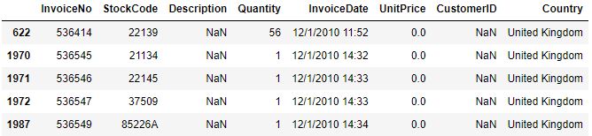
Let’s check the number of missing customers
data[data.Description.isnull()].CustomerID.isnull().value_counts()
True    1454
Name: CustomerID, dtype: int64
and the unit price
data[data.Description.isnull()].UnitPrice.value_counts()
0.0    1454
Name: UnitPrice, dtype: int64
Let’s look at the missing customers
data[data.CustomerID.isnull()].head()

Let’s check the statistics of missing customers
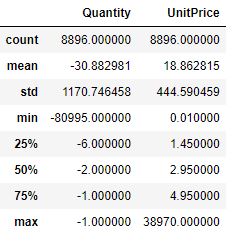
data.loc[data.CustomerID.isnull(), [“UnitPrice”, “Quantity”]].describe()

We can see extreme negative min outliers in the records of missing customers.
Let’s check if we have lowercase “nan”-strings instead of actual nan-values in descriptions
data.loc[data.Description.isnull()==False, “lowercase_descriptions”] = data.loc[
data.Description.isnull()==False,”Description”
].apply(lambda l: l.lower())
data.lowercase_descriptions.dropna().apply(
lambda l: np.where(“nan” in l, True, False)
).value_counts()
False    539724
True        731
Name: lowercase_descriptions, dtype: int64
Let’s check if we have empty “”-strings as well
data.lowercase_descriptions.dropna().apply(
lambda l: np.where(“” == l, True, False)
).value_counts()
False    540455
Name: lowercase_descriptions, dtype: int64
Let’s transform “nan”-strings into nan-variables and drop all missing values
data.loc[data.lowercase_descriptions.isnull()==False, “lowercase_descriptions”] = data.loc[
data.lowercase_descriptions.isnull()==False, “lowercase_descriptions”
].apply(lambda l: np.where(“nan” in l, None, l))
data = data.loc[(data.CustomerID.isnull()==False) & (data.lowercase_descriptions.isnull()==False)].copy()
data.isnull().sum().sum()
0
So there are no missing values left in our data.
Let’s check the min/max time period
data[“InvoiceDate”] = pd.to_datetime(data.InvoiceDate, cache=True)
data.InvoiceDate.max() – data.InvoiceDate.min()
Timedelta('373 days 04:24:00')
print(“Datafile starts with timepoint {}”.format(data.InvoiceDate.min()))
print(“Datafile ends with timepoint {}”.format(data.InvoiceDate.max()))
Datafile starts with timepoint 2010-12-01 08:26:00
Datafile ends with timepoint 2011-12-09 12:50:00
Let’s count all unique invoice numbers
data.InvoiceNo.nunique()
22186
Let’s create the new feature “IsCancelled” to deal with cancelled transactions that start with the capital letter “C”
data[“IsCancelled”]=np.where(data.InvoiceNo.apply(lambda l: l[0]==”C”), True, False)
data.IsCancelled.value_counts() / data.shape[0] * 100
False    97.81007
True      2.18993
Name: IsCancelled, dtype: float64
We can see that 2.2% of total transactions are cancelled.
Let’s check the statistics of these transactions
data.loc[data.IsCancelled==True].describe()
We can see that all cancelled transactions have Quantity<0 and UnitPrice>0.
Let’s drop these transactions
data = data.loc[data.IsCancelled==False].copy()
data = data.drop(“IsCancelled”, axis=1)
data.StockCode.nunique()
3663
So we have got 3663 unique stock codes. Let’s look at the most and least common codes by plotting the histogram
stockcode_counts = data.StockCode.value_counts().sort_values(ascending=False)
fig, ax = plt.subplots(2,1,figsize=(20,20))
sns.barplot(stockcode_counts.iloc[0:20].index,
stockcode_counts.iloc[0:20].values,
ax = ax[0], palette=”Blues_r”)
ax[0].set_ylabel(“Counts”)
ax[0].set_xlabel(“Stockcode”)
ax[0].set_title(“Which stockcodes are most common?”);
sns.distplot(np.round(stockcode_counts/data.shape[0]*100,2),
kde=False,
bins=20,
ax=ax[1], color=”red”)
ax[1].set_title(“How seldom are stockcodes?”)
ax[1].set_xlabel(“% of data with this stockcode”)
ax[1].set_ylabel(“Frequency”);
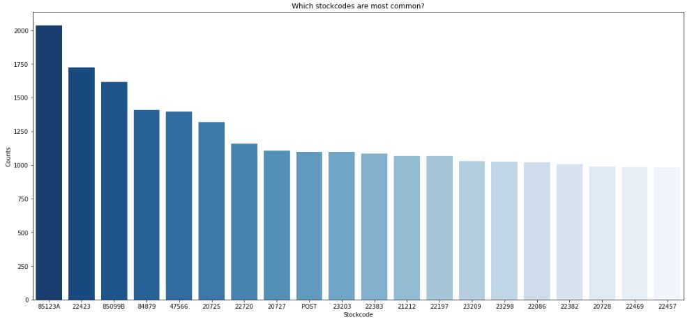
We can see that 85123A is the most common stock code, whereas 22457 is the least common one.

Since most stock codes are very seldom, we conclude that the retailer sells a variety of products without strong secialization.
Let’s count the length and the number of numeric chars in our stock codes
def count_numeric_chars(l):
return sum(1 for c in l if c.isdigit())
data[“StockCodeLength”] = data.StockCode.apply(lambda l: len(l))
data[“nNumericStockCode”] = data.StockCode.apply(lambda l: count_numeric_chars(l))
fig, ax = plt.subplots(1,2,figsize=(20,10))
sns.countplot(data[“StockCodeLength”], palette=”Blues_r”, ax=ax[0])
sns.countplot(data[“nNumericStockCode”], palette=”Blues_r”, ax=ax[1])
ax[0].set_xlabel(“Length of stockcode”)
ax[1].set_xlabel(“Number of numeric chars in the stockcode”);
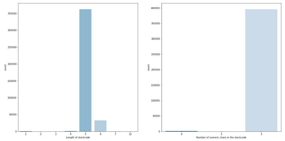
It is clear that the majority of codes consists of 5 numeric chars, but there are other occurences.
Let’s check these outliers
data.loc[data.nNumericStockCode < 5].lowercase_descriptions.value_counts()
postage                       1099
manual                         290
carriage                       133
dotcom postage                  16
bank charges                    12
pads to match all cushions       4
Name: lowercase_descriptions, dtype: int64
Let’s drop all of these occurences:
data = data.loc[(data.nNumericStockCode == 5) & (data.StockCodeLength==5)].copy()
data.StockCode.nunique()
2783
Let’s count the number of unique descriptions
data = data.drop([“nNumericStockCode”, “StockCodeLength”], axis=1)
data.Description.nunique()
2983
Let’s plot the histogram of product descriptions
description_counts = data.Description.value_counts().sort_values(ascending=False).iloc[0:30]
plt.figure(figsize=(30,10))
sns.barplot(description_counts.index, description_counts.values, palette=”Greens_r”)
plt.ylabel(“Counts”)
plt.title(“Which product descriptions are most common?”);
plt.xticks(rotation=90);

We can see that all descriptions consist of uppercase chars. Most common descriptions confirm that the retailers sell different kinds of products.
Let’s count the length and the number of lowercase chars if any.
def count_lower_chars(l):
return sum(1 for c in l if c.islower())
data[“DescriptionLength”] = data.Description.apply(lambda l: len(l))
data[“LowCharsInDescription”] = data.Description.apply(lambda l: count_lower_chars(l))
fig, ax = plt.subplots(1,2,figsize=(20,10))
sns.countplot(data.DescriptionLength, ax=ax[0], color=”Red”)
sns.countplot(data.LowCharsInDescription, ax=ax[1], color=”Red”)
ax[1].set_yscale(“log”)

It appears that almost all descriptions do not have the lowercase chars.
Let’s plot the histogram of descriptions with lowercase chars
lowchar_counts = data.loc[data.LowCharsInDescription > 0].Description.value_counts()
plt.figure(figsize=(15,3))
sns.barplot(lowchar_counts.index, lowchar_counts.values, palette=”Greens_r”)
plt.xticks(rotation=90);
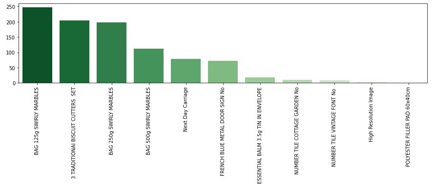
We can see a mix of chars: Next Day Carriage and High Resolution Image.
Let’s compute the ratio of lowercase-to-uppercase letters
def count_upper_chars(l):
return sum(1 for c in l if c.isupper())
data[“UpCharsInDescription”] = data.Description.apply(lambda l: count_upper_chars(l))
data.UpCharsInDescription.describe()
count    362522.000000
mean         22.572291
std           4.354845
min           3.000000
25%          20.000000
50%          23.000000
75%          26.000000
max          32.000000
Name: UpCharsInDescription, dtype: float64
data.loc[data.UpCharsInDescription <=5].Description.value_counts()
Next Day Carriage        79
High Resolution Image     3
Name: Description, dtype: int64
Let’s drop these outliers
data = data.loc[data.UpCharsInDescription > 5].copy()
Let’s plot the histogram of DescriptionLength < 14
dlength_counts = data.loc[data.DescriptionLength < 14].Description.value_counts()
plt.figure(figsize=(20,5))
sns.barplot(dlength_counts.index, dlength_counts.values, palette=”Reds_r”)
plt.xticks(rotation=90);

Descriptions with the length<14 look valid and we should not drop them.
Let’s count unique stock codes and descriptions in our data
data.StockCode.nunique()
2781
data.Description.nunique()
2981
Let’s find out why do we have more descriptions than stock codes.
data.groupby(“StockCode”).Description.nunique().sort_values(ascending=False).iloc[0:10]
StockCode
23236    4
23196    4
23413    3
23244    3
23126    3
23203    3
23209    3
23366    3
23131    3
23535    3
Name: Description, dtype: int64
We still have stock codes with multiple descriptions, for example
data.loc[data.StockCode == “23244”].Description.value_counts()
ROUND STORAGE TIN VINTAGE LEAF    96
STORAGE TIN VINTAGE LEAF           7
CANNISTER VINTAGE LEAF DESIGN      2
Name: Description, dtype: int64
These stock codes look fine.
Let’s count the number of unique customer IDs
data.CustomerID.nunique()
4315
and find out which customers are most common
customer_counts = data.CustomerID.value_counts().sort_values(ascending=False).iloc[0:20]
plt.figure(figsize=(20,10))
sns.barplot(customer_counts.index, customer_counts.values, order=customer_counts.index,palette=”Oranges_r”)
plt.ylabel(“Counts”)
plt.xlabel(“CustomerID”)
plt.title(“Which customers are most common?”);

Let’s check the country list
data.Country.nunique()
37
And which countries are most common?

We can see that the retailer sells almost all products within the UK, followed by many EU countries.
Let’s check the percentage of UK transactions
data.loc[data.Country==”United Kingdom”].shape[0] / data.shape[0] * 100
89.10192031784572
Let’s look at the unit price statistics
data.UnitPrice.describe()
count    362440.000000
mean          2.885355
std           4.361812
min           0.000000
25%           1.250000
50%           1.790000
75%           3.750000
max         649.500000
Name: UnitPrice, dtype: float64
We can see the occurence of zero unit prices.
Let’s check the unit price data content
data.loc[data.UnitPrice == 0].sort_values(by=”Quantity”, ascending=False).head()

It is unclear that zero unit prices are gifts to customers. Let’s drop them
data = data.loc[data.UnitPrice > 0].copy()
and plot the Log-Unit-Price histogram

Let’s focus on lower unit prices
data = data.loc[(data.UnitPrice > 0.1) & (data.UnitPrice < 20)].copy()
and look at quantities
data.Quantity.describe()
count    361608.000000
mean         13.024112
std         187.566510
min           1.000000
25%           2.000000
50%           6.000000
75%          12.000000
max       80995.000000
Name: Quantity, dtype: float64
by plotting the quantity histogram
fig, ax = plt.subplots(1,2,figsize=(20,10))
sns.distplot(data.Quantity, ax=ax[0], kde=False, color=”Blue”);
sns.distplot(np.log(data.Quantity), ax=ax[1], bins=20, kde=False, color=”Blue”);
ax[0].set_title(“Quantity distribution”)
ax[0].set_yscale(“log”)
ax[1].set_title(“Log-Quantity distribution”)
ax[1].set_xlabel(“Natural-Log Quantity”);

Let’s exclude Quantity outliers
data = data.loc[data.Quantity < 55].copy()
and focus on daily product sales
data[“Revenue”] = data.Quantity * data.UnitPrice
data[“Year”] = data.InvoiceDate.dt.year
data[“Quarter”] = data.InvoiceDate.dt.quarter
data[“Month”] = data.InvoiceDate.dt.month
data[“Week”] = data.InvoiceDate.dt.week
data[“Weekday”] = data.InvoiceDate.dt.weekday
data[“Day”] = data.InvoiceDate.dt.day
data[“Dayofyear”] = data.InvoiceDate.dt.dayofyear
data[“Date”] = pd.to_datetime(data[[‘Year’, ‘Month’, ‘Day’]])
grouped_features = [“Date”, “Year”, “Quarter”,”Month”, “Week”, “Weekday”, “Dayofyear”, “Day”,
“StockCode”]
daily_data = pd.DataFrame(data.groupby(grouped_features).Quantity.sum(),
columns=[“Quantity”])
daily_data[“Revenue”] = data.groupby(grouped_features).Revenue.sum()
daily_data = daily_data.reset_index()
daily_data.head(5)

Let’s check the Quantity-Revenue statistics of our daily sales data
daily_data.loc[:, [“Quantity”, “Revenue”]].describe()

We still need to exclude outliers by considering 90% of our sales data
low_quantity = daily_data.Quantity.quantile(0.01)
high_quantity = daily_data.Quantity.quantile(0.99)
print((low_quantity, high_quantity))
(1.0, 88.48000000001048)
low_revenue = daily_data.Revenue.quantile(0.01)
high_revenue = daily_data.Revenue.quantile(0.99)
print((low_revenue, high_revenue))
(0.78, 204.0)
samples = daily_data.shape[0]
daily_data = daily_data.loc[
(daily_data.Quantity >= low_quantity) & (daily_data.Quantity <= high_quantity)] daily_data = daily_data.loc[ (daily_data.Revenue >= low_revenue) & (daily_data.Revenue <= high_revenue)]
samples – daily_data.shape[0]
5258
That’s the amount of lost data entries.
Let’s look at the sales data without outliers
fig, ax = plt.subplots(1,2,figsize=(20,10))
sns.distplot(daily_data.Quantity.values, kde=True, ax=ax[0], color=”Green”, bins=30);
sns.distplot(np.log(daily_data.Quantity.values), kde=True, ax=ax[1], color=”Green”, bins=30);
ax[0].set_xlabel(“Number of daily product sales”);
ax[0].set_ylabel(“Frequency”);
ax[0].set_title(“How many products are sold per day?”);

We can see that the daily sales distributions are right skewed in that lower values (small quantities of products) are more common. In addition, multiple modes indicate several periodic sales anomalies to be examined separately.
Conclusion
We have discussed the use-case of retail analytics and related BI insights to analyze sales performance and optimize processes. This analytics offers the following opportunities pertaining to online sales:
- Using these insights, retailers can improve both the sales force performance as well as their overall profitability.
- It takes into account the effect of seasonality, any executed Ad-campaigns, running Sales Promotion events or any competitor’s activity that can impact sales. These insights help retailers in stocking the inventory accordingly.
- It uncovers associations between items; it may be because these are complementary products or have a tendency to be bought together. With the help of these insights, the store owners can create a tailored assortment of products and play with the margins by clubbing expensive (high margin) items with less selling discounted items. A correlation between the number of users in a family and identifying cross-sell & up-sell opportunities is key to driving sales.
- Customer Trend Identification To Drive The Pricing & Promotion Plan. It allows e-commerce players to push out relevant offers to each customer at every stage of their buyer’s journey.
- Analytics is also very crucial to analyse the success factors driving a product’s sale. A benchmarking of these factors could go a long way in building a successful new product strategy.
- It is capable enough to analyse if a competitor enjoys some unique advantage or has some gap in their product portfolio. Also, a BI system can draw insights from the impact analysis of the competitors’ pricing & promotion events.


Leave a comment