
Featured Photo by Harsch Shivam
- Community Forum Q&A, FAQ, Tips, Ideas
- Bayes’ Formula Demystified
- Non-Linear Regression Analysis
- Posts of Interest
- XebiaLabs to Update Periodic Table of DevOps Tools
- The Content Marketing (CM) in a Nutshell
- A Start-Up Marketing Plan
- Advanced ML/AI: BTC-USD Price Prediction with LSTM Keras
- Cloud-Native Tech Autumn 2022 Fair
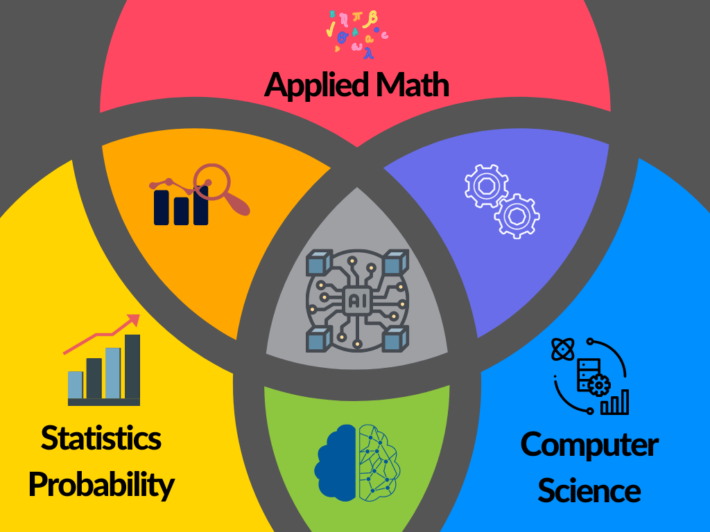
The discipline of Data Science (DS) sits at the interface between Technology, the quantitative sciences (such as mathematics, statistics, computer science) and engineering across various business applications and sectors. This page aims to review new methods, research findings, opinions, hypothesis articles and poster presentations on all relevant aspects of DS.
As DS bridges data analytics, statistics, business intelligence (BI), artificial intelligence (AI)-powered technology and data engineering, the page is focused on applying advanced predictive analytics techniques and scientific principles to extract valuable information from data for business decision-making, strategic planning and other uses. It’s increasingly critical to businesses: The insights that data science generates help organizations increase operational efficiency, identify new business opportunities and improve marketing and sales programs, among other benefits. Ultimately, they can lead to competitive advantages over business rivals.
An effective DS team may include the following specialists: Data engineer, data analyst, Machine Learning (ML) engineer, data visualization analyst, data translator, and data architect.
The following most recent business applications drive a wide variety of DS use cases in organizations globally:
- HealthTech
- E-Commerce
- Customer experience
- Risk management
- FinTech
- Stock trading
- Digital marketing
- Industrial IoT applications
- Logistics & supply chain management
- Image/Speech Recognition
- Cybersecurity
- LegalTech
Community Forum Q&A, FAQ, Tips, Ideas
- What are the advantages of stochastic block models?
Finding communities in complex networks is a challenging task and one promising approach is the Stochastic Block Model (SBM). But the influences from various fields led to a diversity of variants and inference methods. Therefore, a comparison of the existing techniques and an independent analysis of their capabilities and weaknesses is needed.
- What is the probability that a surfer will hit a particular website?
This is the Random Web Surfer Page Rank Algorithm.
Read more here.
- What’s OCR data extraction?
OCR is an acronym for Optical Character Recognition. It is a powerful technology that can transform scanned documents or image files into easily accessible and editable data. It can extract text from digital files, scanned documents (handwritten or printed documents), and PDFs. This is an actual application for our MNIST Digits Classifier.
Read more here about OCR of Handwritten digits | OpenCV.
- I am facing serious trouble on understanding ‘Database Relationships’.
Database relationships are associations between tables that are created using join statements to retrieve data. One of the advantages of a relational database (RDBMS) is that you can relate the data held in different tables. There are three types of relationships between the data: one-to-one, one-to-many, and many-to-many. You can define SQL statements for joins, and create relationships between parent and child objects. The parent is the existing object and the child is the object that you are create. Tip: You can manage relationships in Power BI. Read more: Power BI for Data Science.
- Is pursuing a master’s degree for quantum engineering worth it as opposed to AI or data science? What are the job prospects?
AI belongs to data science, and the latter implies large-scale deployment that would requires quantum computing by no means.
Quantum computing is a rapidly accelerating field with the power to revolutionize artificial intelligence (AI) and machine learning (ML). As the demand for bigger, better, and more accurate AI and ML accelerates, standard computers will be pushed to the limits of their capabilities.
- What are the steps to start a career on big data and data science analysis and so on?
- Read this blog: A Roadmap from Data Science to BI via ML
- How can vector databases like Pine cone improve anomaly detection?
The Pinecone vector database makes it easy to build high-performance vector search applications. ML techniques can offer a helpful representation of complex data by transforming it into vector embeddings.
As good as vector databases are in finding similar objects, they can also find objects that are distant or dissimilar from an expected result. These anomalies are valuable in applications used for threat assessment, fraud detection, and IT Operations. It’s possible to identify the most relevant anomalies for further analysis without overwhelming resources with a high rate of false alarms. See the example code.
- How do you calculate the least squares line in two dimensions?
This is all about Linear least squares fitting of a two-dimensional data.
Matlab polyfit is another option to explore.
- Is it worth studying data analytics/data science anymore, with AI being able to handle and analyse data so much faster, like the code interpreter that ChatGPT is releasing?
Yes, absolutely. Data analytics and data science are still essential skills in the modern world. AI can help speed up the process of data analysis, but it can’t replace the need for human expertise. As AI and machine learning become more advanced, they can help automate more of the data analysis process, but they still need humans to interpret the results and make decisions. Additionally, data analytics and data science are more than just analyzing data; they involve understanding the context and implications of the data, as well as being able to communicate the results effectively.
- What are your thoughts on the upcoming online master of science program in data science at the University of Colorado Boulder?
I think the University of Colorado Boulder’s online Master of Science program in Data Science is an exciting opportunity for students who are interested in furthering their education in this field. The program promises to provide a comprehensive and rigorous education in data science, and it is likely to be a great way for students to gain the skills and knowledge they need to succeed in the field. Additionally, the online format of the program makes it accessible to a wider range of students, regardless of their location or other commitments.
- Can you use an SVM classifier on categorical data before converting it into binary features using binarization or not using any pre-processing at all for the same dataset?
Yes, it is possible to use an SVM classifier on categorical data before converting it into binary features using binarization or not using any pre-processing at all for the same dataset. However, in order to get the best results, it is recommended to pre-process the data to convert the categorical features into numerical features. This can be done by using one-hot encoding or label encoding.
- What are some affordable online master’s programs in big data analytics offered by reputable universities in the UAE?
- American University of Sharjah: Master of Science in Data Analytics
- University of Dubai: Master of Science in Big Data Analytics
- Heriot-Watt University Dubai: MSc in Data Science and Analytics
- Middlesex University Dubai: MSc in Big Data Analytics
- American University in the Emirates: Master of Science in Data Science
- Skyline University College: Master of Science in Big Data Analytics
- University of Wollongong Dubai: MSc in Data Analytics and Business Intelligence
- Manipal University Dubai: MSc in Big Data Analytics
- Zayed University: Master of Science in Data Science and Analytics
- University of Sharjah: Master of Science in Data Science and Analytics
- Hey guys, does anybody know anything about Infobel Pro? I am a startup, and I am about to choose a B2B data provider and wanted to get some opinions about them because it seems they have the largest amount of data (specifically Asia + EU).?
Infobel Pro is an online directory of businesses and individuals from around the world. It provides detailed information about each listing, such as contact information, business activities, and more. The directory is searchable and can be used to find business contacts, customers, and suppliers. It also offers a variety of services, such as email marketing, lead generation, and more.
- What are your thoughts on Big Data Analytics and Machine Learning by Pankaj Tiwari?
Pankaj Tiwari: Future of AI and Machine Learning with Explainable AI (XAI)
Read more about the techniques like Layerwise Relevance Propagation and Deep Taylor Series to build indicative XAI.
- What software tools do Data Scientists use to process large datasets into useful information?
- Apache Hadoop: Apache Hadoop is an open source software framework for distributed storage and processing of large datasets. It is designed to scale up from single servers to thousands of machines, each offering local computation and storage.
- Apache Spark: Apache Spark is an open source data processing framework for analyzing large datasets. It is designed for speed, ease of use, and scalability.
- Apache Pig: Apache Pig is a high-level data-flow language and execution framework for parallel computation. It allows users to write complex data-processing pipelines using a simple scripting language.
- Apache Flink: Apache Flink is an open source distributed data processing framework. It is designed to process data in parallel and supports streaming and batch processing.
- Python: Python is a popular programming language for data science. It is powerful, flexible, and easy to learn. It is used to build powerful data analysis and machine learning models.
- R: R is a programming language and software environment for statistical computing and graphics. It is used for data analysis, machine learning, and visualization.
- Tableau: Tableau is a powerful data visualization tool. It allows users to quickly explore and analyze large datasets. It is used for data discovery and communication.
- What are some good MSc or MBA courses in Big Data Analytics from India?
- MSc in Data Science and Analytics from Manipal University
- MSc in Data Science from BITS Pilani
- MBA in Big Data Analytics from ICFAI Business School
- MBA in Business Analytics from Great Lakes Institute of Management
- MSc in Business Analytics from Amrita Vishwa Vidyapeetham
- MSc in Data Science and Business Analytics from Vellore Institute of Technology
- MSc in Data Science from IIIT Bangalore
- MBA in Big Data Analytics from Indian Institute of Management, Ahmedabad
- MSc in Business Analytics from Indian Institute of Management, Kozhikode
- MSc in Business Analytics from Symbiosis International University
- What is the difference between a medical researcher, a basic scientist, and a clinical researcher?
Step 1: Calculate the mean (μ) and standard deviation (σ) of the data set.
Step 2: Subtract the mean from the raw score to get the difference (x – μ).
Step 3: Divide the difference by the standard deviation (x – μ) / σ.
Step 4: The result is the Z-score.
- What is automatic speech recognition and can it be used for transcription purposes in research interviews?
Automatic speech recognition (ASR) is a technology that enables computers to recognize and interpret spoken language. It can be used to convert spoken language into text, and it is used in a variety of applications, such as voice-enabled search and command, voice-controlled devices, and automated call routing. ASR can be used for transcription purposes in research interviews, as it can accurately convert spoken language into text. This can be useful for researchers who need to analyze the content of interviews quickly and accurately.
- What are the suggested tools used for magazine research?
- Google Trends: This tool can be used to track the popularity of topics and keywords related to your magazine.
- Social Media Analytics: Tools such as Hootsuite and Sprout Social can be used to track the engagement and reach of your magazine’s content on social media.
- Survey Tools: Services like SurveyMonkey and Typeform can be used to survey readers to better understand their interests and preferences.
- Competitor Analysis: Tools such as SimilarWeb can be used to compare your magazine’s performance with other magazines in the same industry.
- Industry Reports: Reports from organizations such as the Magazine Publishers Association can provide valuable insights into the magazine industry.
- What are the different courses offered by the Welingkar Institute of Management and Technology? What are the benefits of each course?
The Welingkar Institute of Management and Technology offers a range of courses in the field of management and technology. These include:
- MBA in Retail Management: This course focuses on the understanding of the retail sector, its operations, and the strategies for success. It equips the students with the necessary skills to manage retail operations and build a successful career in the sector.
- MBA in Business Analytics: This course provides an in-depth understanding of analytics and its application in the business world. It helps the students to develop their analytical skills and apply them to solve real-world business problems.
- MBA in Banking and Financial Services: This course provides the students with an in-depth knowledge of the banking and financial services industry. It helps the students to develop their skills in the areas of banking, finance, investments, and risk management.
- MBA in Digital Business: This course helps the students to understand the digital business landscape and the strategies for success in the digital world. It equips the students with the necessary skills to manage digital operations and build a successful career in the sector.
- MBA in Entrepreneurship: This course provides the students with an understanding of the entrepreneurial process and the strategies to build a successful business. It helps the students to develop their skills in the areas of innovation, strategy, and leadership.
Benefits of these courses:
- MBA in Retail Management: This course provides the students with an in-depth knowledge of the retail sector, its operations, and the strategies for success. It equips the students with the necessary skills to manage retail operations and build a successful career in the sector.
- MBA in Business Analytics: This course helps the students to develop their analytical skills and apply them to solve real-world business problems. It provides the students with an understanding of the analytics landscape and the strategies to use analytics to make better business decisions.
- MBA in Banking and Financial Services: This course helps the students to develop their skills in the areas of banking, finance, investments, and risk management. It provides the students with an understanding of the banking and financial services industry and the strategies for success in the sector.
- MBA in Digital Business: This course equips the students with the necessary skills to manage digital operations and build a successful career in the sector. It provides the students with an understanding of the digital business landscape and the strategies for success in the digital world.
- MBA in Entrepreneurship: This course helps the students to develop their skills in the areas of innovation, strategy, and leadership. It provides the students with an understanding of the entrepreneurial process and the strategies to build a successful business.
- Why is ‘big data’ important to software developers?
Big data is important to software developers because it provides them with a wealth of information that can be used to develop better software. By analyzing large sets of data, software developers can gain insights into customer behavior, market trends, and user preferences, which can help them create more targeted and effective software solutions. Additionally, big data can be used to improve software performance, identify and fix bugs, and ensure that software is secure and reliable.
- What are some basic courses for an MA in public policy and governance?
- Introduction to Public Policy and Governance
- Public Policy Analysis
- Research Methods in Public Policy
- Economics for Public Policy
- Public Budgeting and Finance
- Public Management and Leadership
- Social Policy Analysis
- Public Law and Regulation
- Comparative Public Policy
- International and Global Governance
- How can time series data be visualized using RStudio and ggplot2 (or other methods)?
Check out this link:
Webscraping in R – The IMDb ETL Showcase
- What is the most important course to take during an MSBA program?
Answer: Data Science
Read more here:
A Roadmap from Data Science to BI via ML
Masters in Business Analytics is a perfect blend of Data Science, Information Theory, Business Intelligence and Computer Science. Its major aim is to change heavy data into actionable intelligence by using different quantitative and statistical methods. To put it simply, Masters in Business Analytics is concerned with mining data in order to get particular business objectives; instead of focusing on measuring past performance, it’s more concerned with predictive and prescriptive techniques.
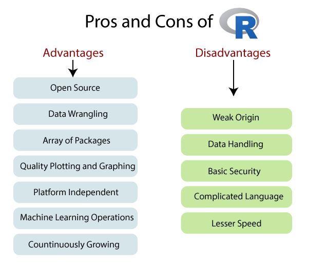
- What are the advantages of using Python over R when working with Data Science/Big Data Analytics projects?
- Python is a general-purpose language, meaning it can be used for a wide variety of tasks, including data science and big data analytics. R is a domain-specific language, meaning it is designed for statistical computing and graphics.
- Python has a larger user base than R, meaning there is a larger community of developers and support available.
- Python is easier to learn and use than R, making it more accessible to beginners.
- Python has a larger library of packages and modules than R, meaning it can be used for a wider range of tasks.
- Python is faster than R, making it more suitable for large-scale data analysis and machine learning tasks.
- Python is more versatile than R, allowing for the integration of other programming languages and tools.
- What is your strategy to avoid type I or II error when doing hypothesis testing with small or large samples?
- When dealing with small samples, it is important to use a large enough sample size to ensure that the results are statistically significant. This can be done by using a power analysis to determine the necessary sample size.
- When dealing with large samples, it is important to use a conservative significance level (e.g. 0.01 or 0.001) in order to reduce the chances of a Type I error.
- In both cases, it is important to use a well-defined null hypothesis and an appropriate statistical test to ensure that the results are valid.
- What are the benefits of using Tensorflow over other frameworks like PyTorch, Keras, or Theano?
- TensorFlow has a large community and is well-supported with tutorials, documentations, and other resources.
- TensorFlow is highly scalable, allowing for distributed training and deployment across multiple machines.
- TensorFlow’s graph-based computation model makes it easier to debug and visualize complex networks.
- TensorFlow is designed for production use, allowing for easy deployment of trained models.
- TensorFlow has built-in support for automatic differentiation, making it easier to implement complex architectures.
- TensorFlow’s high-level APIs make it easier to quickly build and train models, allowing for faster experimentation.
Read more about Tensorflow
99% Accurate Breast Cancer Classification using Neural Networks in TensorFlow 2.11.0
- What are some tips for using pandas as a data source in Tableau?
- Make sure the data is in the right format for Tableau. Tableau works best with data that is in a tabular format, so make sure that the data is in a tidy format with each variable in a separate column.
- Use the Pandas melt() function to transform your data into long format. This will make it easier to work with in Tableau.
- Use the Pandas groupby() function to aggregate and summarize your data. This will give you a better understanding of your data and make it easier to visualize in Tableau.
- Use the Pandas pivot_table() function to reshape your data. This will allow you to create more complex visualizations in Tableau.
- Use the Pandas to_csv() function to save your data in a CSV format. This will make it easier to import into Tableau.
- How do you become an entry level data scientist? How much could one earn per month from such a role if hired immediately after graduation (BS, statistics)?
To become an entry level data scientist, you will need to have a strong background in mathematics and statistics, as well as experience with coding and data analysis. You should also have a good understanding of machine learning algorithms and techniques. Additionally, you should have a strong portfolio of data science projects and be able to demonstrate your analytical and problem-solving skills.
The salary for an entry-level data scientist can vary depending on the company and the location. Generally speaking, entry-level data scientists can earn an average of $60-90k per year. If hired immediately after graduation, the salary could be lower, starting at around $50k per year.
- What are some good and bad examples of charts?
Good Examples:
- Bar Chart: A bar chart is a great way to visually compare different categories of data. It can be used to compare values over time, or to compare different items within a category.
- Line Chart: A line chart is a great way to visualize trends over time. It can be used to track changes in a single variable over time, or to compare multiple variables over time.
- Pie Chart: A pie chart is a great way to quickly show the relative proportions of different categories. It can be used to compare the parts of a whole, or to compare the proportions of different items within a category.
Bad Examples:
- 3D Pie Chart: A 3D pie chart is difficult to read and can be misleading. It can make it difficult to compare different categories, or to accurately read the data.
- Stacked Bar Chart: A stacked bar chart can be difficult to read and can be misleading. It can make it difficult to compare different categories, or to accurately read the data.
- Radar Chart: A radar chart is difficult to read and can be misleading. It can make it difficult to compare different categories, or to accurately read the data.
Read more use-cases of data visualization in Python
- What is the biggest challenge of big data in 2023?
The biggest challenge of big data in 2023 is managing and analyzing the sheer volume of data. As data continues to increase exponentially, businesses must be able to effectively store, process, and analyze the data in order to derive meaningful insights. Additionally, organizations must be able to identify the most relevant data and use the insights to make informed decisions. Furthermore, they must be able to do this quickly and accurately in order to stay competitive.
Solution: multi-cloud AIOps
Read more AI-relevant Posts.
- How can data accuracy be ensured?
- Validate Data: Data validation is the process of ensuring that data is accurate, complete, and valid before it is stored in a database.
- Quality Control: Quality control is the process of ensuring that data is accurate and complete by verifying the accuracy, completeness, and consistency of data.
- Use Automated Tools: Automated tools such as data quality tools can help to ensure data accuracy by automatically detecting and correcting errors in data.
- Regular Audits: Regular audits of data can help to identify any discrepancies and errors in data.
- Establish Clear Data Definitions: Establishing clear definitions for data and ensuring that everyone follows them can help to ensure data accuracy.
- Train Employees: Training employees on data accuracy and data entry best practices can help to ensure data accuracy.
Read more data QC relevant Posts.
- How Uber uses Machine Learning?
Uber uses machine learning in a variety of ways. One example is in predicting demand for its services. By analyzing past data, Uber can predict where and when demand for its services will be highest and adjust prices accordingly. This helps to ensure that drivers are able to make more money while also providing customers with an affordable ride.
Uber also uses machine learning to detect fraud. By analyzing past data, Uber can detect patterns of fraudulent activity, such as riders using stolen credit cards or drivers engaging in illegal activities. This helps to ensure that Uber’s services are safe and secure for both riders and drivers.
Finally, Uber uses machine learning to improve its routing algorithms. By analyzing past data, Uber can more accurately predict the fastest route for drivers and riders, helping to reduce travel time and increase customer satisfaction.
- Is Prompt engineering the new hottest tech job?
No, prompt engineering is not the new hottest tech job. It is a relatively new field, but there are many other tech jobs that are more in demand. Some of these include software engineering, data science, artificial intelligence, and cybersecurity, as explained below
- In Healthcare Machine Learning, what is the primary advantage of using Federated Learning?
The primary advantage of using Federated Learning in Healthcare Machine Learning is that it allows for the secure and privacy-preserving sharing of data across multiple parties. Federated Learning allows for the training of models on distributed data without having to move or store the data in a central location. This helps to ensure that the data remains secure and private, while still allowing for the development of powerful machine learning models.
A Roadmap from Data Science to BI via ML
- What are the pros and cons of switching to PyTorch from Theano/TensorFlow for deep learning research?
Pros:
- PyTorch is much easier to use than Theano or TensorFlow. It has a much more intuitive and user-friendly API, making it easier to learn and use.
- PyTorch is much faster than Theano or TensorFlow. It has a dynamic computation graph that allows for faster training and inference.
- PyTorch has better support for distributed training, allowing for faster training on multiple machines.
- PyTorch has a much larger community and more resources available, making it easier to find help or tutorials when needed.
Cons:
- PyTorch is relatively new, so it may not have as many features as Theano or TensorFlow.
- PyTorch does not have as much support for production-level deployment as Theano or TensorFlow.
- PyTorch is not as widely used as Theano or TensorFlow, so there may be fewer community resources available.
- What is the best way to get into data analysis for someone with no background or education in computer science or mathematics?
- Start with the quick hands-on plunge into basics of data analysis
2. Follow the Python/R open-source code examples available on Kaggle and GitHub
3. Share your findings and acquired knowledge with the learning community by publishing blogs and participating in relevant discussion forums.
Explore more
A Roadmap from Data Science to BI via ML
The 5-Step Tech Blogging Roadmap
- What are some examples of Power BI visuals that can be used to analyze data distribution?
- Histogram: A histogram is a graphical representation of data distribution that shows the frequency of a particular variable in a set of data.
- Box and Whisker Plot: A box and whisker plot is a graphical representation of data distribution that shows the median, quartiles, and range of a data set.
- Scatter Plot: A scatter plot is a graphical representation of data distribution that shows the relationship between two variables.
- Pareto Chart: A Pareto chart is a graphical representation of data distribution that shows the relative importance of different categories of data.
- Waterfall Chart: A waterfall chart is a graphical representation of data distribution that shows the cumulative effect of different categories of data.
- Can I do an MS in GIS after a bachelor’s in environmental science?
Yes, you can. GIS is a popular tool used in environmental science, and many universities offer GIS programs that are tailored to environmental science students.
See the excellent example of the relevant MS project
ML/AI Wildfire Prediction using Remote Sensing Data
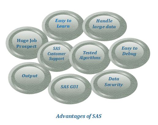
- What are the benefits of SAS and R for data science? Which one has more job opportunities in the future and why?
- How can businesses use data analytics to make more informed decisions?
There are several benefits to data-driven decision-making:
- Enhanced accuracy of decisions
- Cost savings and operational efficiency
- Create personalized customer experiences
- Agility to stay ahead of the competition
- How does the current ChatGPT work and process data?
- ChatGPT is the latest language model from OpenAI and represents a significant improvement over its predecessor GPT-3. Similarly to many Large Language Models (LLMs), ChatGPT is capable of generating text in a wide range of styles and for different purposes, but with remarkably greater precision, detail, and coherence. It is designed with a strong focus on interactive conversations.
- ChatGPT provides a response based on the context and intent behind a user’s question. You can’t, for example, ask Google to write a story or ask Wolfram Alpha to write a code module, but ChatGPT can do these sorts of things.
References
- Which software can I use for data mining in medical record?
OSP – HEALTHCARE DATA MINING SOFTWARE SOLUTIONS
- MySQL vs PostgreSQL vs SQLite – What is the difference?
MySQL vs PostgreSQL vs SQLite – 3 RDBMSs
MySQL is one of the most popular open-source and large-scale RDBMS systems out there. Unlike SQLite, it employs a server/client architecture.
MySQL is owned and maintained by Oracle.
Like MySQL, PostgreSQL uses a client/server database model and the server process that handles the client communications.
Unlike MySQL, PostgreSQL supports materialized views (cached views) resulting in faster frequent access to big and active tables.
In terms of popularity, MySQL is way ahead of PostgreSQL and SQLite, but one must consider the use case and features before making it the de-facto choice.
SQLite is serverless, suitable for Low-Medium Traffic Websites, IoT and Embedded Devices, Testing and Development.
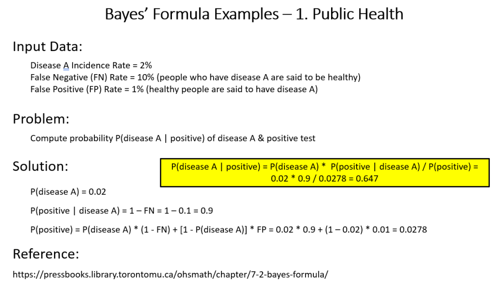
Bayes’ Formula Demystified
Non-Linear Regression Analysis
Nonlinear regression is a form of regression analysis in which data is fit to a model and then expressed as a mathematical function. Simple linear regression relates two variables (X and Y) with a straight line (y = mx + b), while nonlinear regression relates the two variables in a nonlinear (curved) relationship.
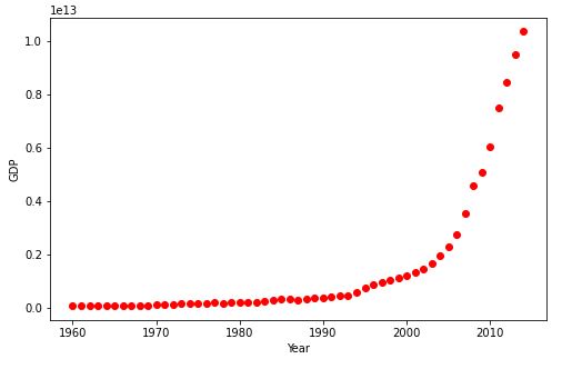
Let’s learn about non-linear regressions by considering a few examples in Python. The scikit-learn library contains the simplified example of 1D regression using linear, polynomial and RBF kernels, as shown below. As a real-worls example, we fit a non-linear model to the datapoints corrensponding to China’s GDP from 1960 to 2014.

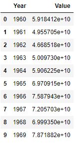
China’s GDP Example
Let’s consider the China’s GDP Kaggle Dataset to test the non-linear regression algorithm
Import and install libraries
import numpy as np
import pandas as pd
!pip install wget
Read the csv file
df = pd.read_csv(“YourPath/china_gdp.csv”)
df.head(10)
Let’s plot the data
import matplotlib.pyplot as plt
%matplotlib inline
plt.figure(figsize=(8,5))
x_data, y_data = (df[“Year”].values, df[“Value”].values)
plt.plot(x_data, y_data, ‘ro’)
plt.ylabel(‘GDP’)
plt.xlabel(‘Year’)
plt.show()
Let’s introduce the non-linear sigmoid function
X = np.arange(-5.0, 5.0, 0.1)
Y = 1.0 / (1.0 + np.exp(-X))
plt.plot(X,Y)
plt.ylabel(‘Dependent Variable’)
plt.xlabel(‘Indepdendent Variable’)
plt.show()
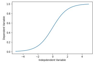
def sigmoid(x, Beta_1, Beta_2):
y = 1 / (1 + np.exp(-Beta_1*(x-Beta_2)))
return y
beta_1 = 0.10
beta_2 = 1990.0
Logistic function
Y_pred = sigmoid(x_data, beta_1 , beta_2)
Let’s plot initial prediction against datapoints
plt.plot(x_data, Y_pred*15000000000000.)
plt.plot(x_data, y_data, ‘ro’)

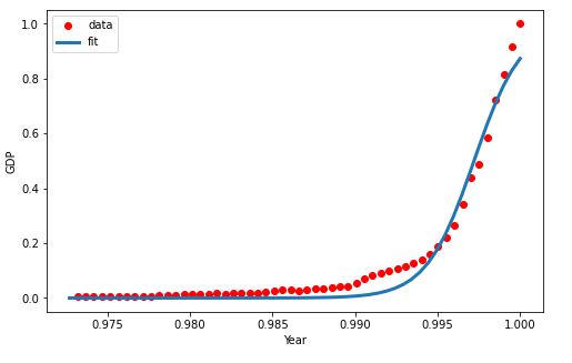
Lets normalize our data
xdata =x_data/max(x_data)
ydata =y_data/max(y_data)
Let’s perform non-linear curve fitting
from scipy.optimize import curve_fit
popt, pcov = curve_fit(sigmoid, xdata, ydata)
And print the final parameters
print(” beta_1 = %f, beta_2 = %f” % (popt[0], popt[1]))
beta_1 = 690.451712, beta_2 = 0.997207
x = np.linspace(1960, 2015, 55)
x = x/max(x)
plt.figure(figsize=(8,5))
y = sigmoid(x, *popt)
plt.plot(xdata, ydata, ‘ro’, label=’data’)
plt.plot(x,y, linewidth=3.0, label=’fit’)
plt.legend(loc=’best’)
plt.ylabel(‘GDP’)
plt.xlabel(‘Year’)
plt.show()
Let’s split data into the train and test sets
msk = np.random.rand(len(df)) < 0.8
train_x = xdata[msk]
test_x = xdata[~msk]
train_y = ydata[msk]
test_y = ydata[~msk]
Let’s build the model using the train set
popt, pcov = curve_fit(sigmoid, train_x, train_y)
Predict using test set
y_hat = sigmoid(test_x, *popt)
Perform evaluation
print(“Mean absolute error: %.2f” % np.mean(np.absolute(y_hat – test_y)))
print(“Residual sum of squares (MSE): %.2f” % np.mean((y_hat – test_y) ** 2))
from sklearn.metrics import r2_score
print(“R2-score: %.2f” % r2_score(y_hat , test_y) )
Mean absolute error: 0.03
Residual sum of squares (MSE): 0.00
R2-score: 0.96
- An Intro to Graph Algorithms in R
- Python Data Science for Real Estate & REIT Amsterdam: (Auto) EDA, NLP, Maps & ML
- Titanic Benchmark Hypothesis Testing in Disaster Risk Management: (Auto)EDA, ML, HPO & SHAP
- Walmart Weekly Sales Time Series Forecasting using SARIMAX & ML Models
- Time Series Data Imputation, Interpolation & Anomaly Detection
Posts of Interest
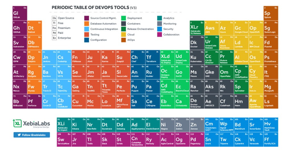
XebiaLabs to Update Periodic Table of DevOps Tools
#ContinuousDelivery#XLPeriodicTable#DevOps
Version 4 of the industry’s most popular DevOps market landscape tool, the Periodic Table of DevOps. Selected Vendors: Snowflake, Moogsoft, Instana, DataDog, GitLab, among others.
The Content Marketing (CM) in a Nutshell
CM is a strategic marketing approach focused on creating and distributing valuable, relevant, and consistent content to attract and retain a clearly defined audience — and, ultimately, to drive profitable customer action.
Benefits of CM:
* Grow brand awareness
* Drive organic visitors
* Generate sales leads
* Build trust
* Earn customer loyalty
* Create demand
The 3 key elements of effective CM are:
- Move your audience
- Earn your audiences attention
- Have a spark

A Start-Up Marketing Plan

Investor FAQ
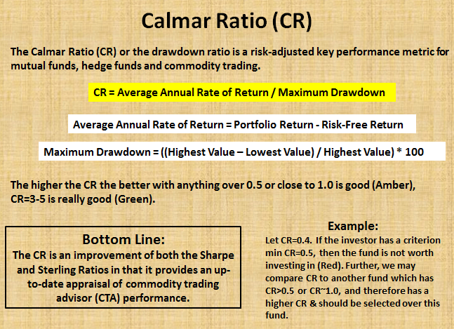
The Calmar Ratio (CR) or the drawdown ratio is a risk-adjusted key performance metric for mutual funds, hedge funds and commodity trading. In fact, it measures the return per unit of risk and lets the investor decide whether the given amount of return is worth it at the given level of risk or not. Calmar is short for California Managed Accounts Report and is very similar to MAR ratio. The CR was first published in 1991. It is most similar to the Sterling ratio in its calculation, it takes the average annual compounded rate of return and divides it by the maximum drawdown for that same time period, usually over a period of 3 years. The higher the CR the better with anything over 0.5 or close to 1.0 is good (Amber), CR=3-5 is really good (Green).
Let’s consider a fund started 3 years ago. It reached a value of $2 mln but went as low as $1.5 mln. Over this period the average annual return was 10%. In this example, the CR should help in evaluating whether the fund is worth investing. The outcome is given below:

It appears that the risk-adjusted ratio is 0.4. If the investor has a criterion of a minimum CR of 0.5 [21], then the fund is not worth investing in (Red). Further, we may compare CR to another fund which has CR>0.5 or CR~1.0, and therefore has a higher risk-adjusted return and should be selected over this fund.
The CR is an improvement of both the Sharpe and Sterling Ratios in that it provides an up-to-date appraisal of commodity trading advisor (CTA) performance.
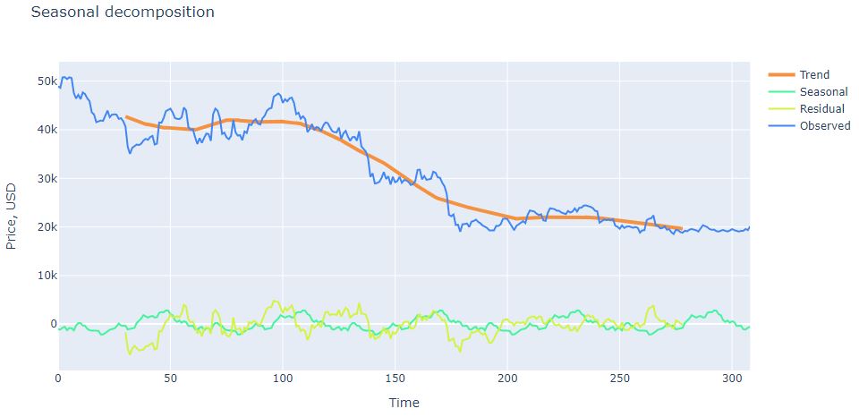
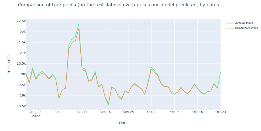
Advanced ML/AI: BTC-USD Price Prediction with LSTM Keras

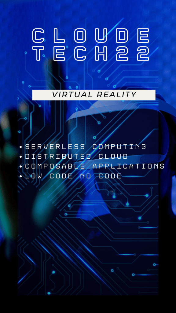
Cloud-Native Tech Autumn 2022 Fair


Leave a comment