
Featured Image Design Template via Canva.
- Amsterdam’s (AMS) Real Estate Market is experiencing an resurgence, with property prices soaring by double-digits on an yearly basis since 2013.
- Can data science help us understand where we stand in the AMS housing market? Read more here.
- Following the recent ML studies, let’s take a closer look at the city’s rental market landscape using data science in Python.
- Project 1: Amsterdam Inside Airbnb
From the project website: http://insideairbnb.com/about/
Inside Airbnb is a mission driven project that provides data and advocacy about Airbnb’s impact on residential communities.
We work towards a vision where data and information empower communities to understand, decide and control the role of renting residential homes to tourists.
- Project 2: Amsterdam House Price Prediction
The housing prices have been obtained from Pararius.nl as a snapshot in August 2021 (courtesy of Pararius). The original data provided features such as price, floor area and the number of rooms. The data has been further enhanced by utilizing the Mapbox API to obtain the coordinates of each listing.
Table of Contents
- An Environment Setup
- About Input Datasets in Projects 1-2
- Project 1: Interactive Data Analysis with ITables
- Projects 1-2: Basic Statistical Data Analysis
- Projects 1-2: Exploratory Data Analysis (EDA) & ML
- Project 1: SweetViz AutoEDA
- Project 1: AutoViz AutoEDA
- Project 1: Geospatial EDA
- Project 1: NLP Wordcloud Images
- Project 1: ML Regression of Review Scores
- Project 2: Tuned RF Regression of Prices
- Conclusions
- Explore More
- References
- Embed Socials
- Infographics
An Environment Setup
- Set up a lean, robust data science environment with Miniconda and Conda-Forge
- Download and install Miniconda
- conda create -n my-conda-env
- conda install jupyter
- jupyter notebook
- For installing multiple packages from the command line, just pass them as a space-delimited list, e.g.:
- pip install package1, package2, …
- conda deactivate (exit)
- Jupyter Notebook: Setting up the working directory YOURPATH
import os
os.chdir('YOURPATH')    # Set working directory
os. getcwd()
- Basic Python imports and installations
import numpy as np
import pandas as pd
import seaborn as sns
sns.set()
import matplotlib.pyplot as plt

import os
import warnings
warnings.simplefilter(action='ignore', category=FutureWarning)

#to make the interactive maps
import folium
from folium.plugins import FastMarkerCluster
import geopandas as gpd
from branca.colormap import LinearColormap

#to make the plotly graphs
import plotly.graph_objs as go
import chart_studio.plotly as py
from plotly.offline import iplot, init_notebook_mode
import cufflinks
cufflinks.go_offline(connected=True)
init_notebook_mode(connected=True)

#text mining
from nltk.tokenize import word_tokenize
from nltk.corpus import stopwords
import re
from sklearn.feature_extraction.text import TfidfVectorizer, CountVectorizer
from wordcloud import WordCloud
About Input Datasets in Projects 1-2
- Project 1: File descriptions in the netherlands/Amsterdam folder:
- listings.csv: Detailed Listings data
- calendar.csv: Detailed Calendar Data
- reviews.csv: Detailed Review Data
- listings.csv: Summary information and metrics for listings in Amsterdam (good for visualizations).
- reviews.csv: Summary Review data and Listing ID (to facilitate time based analytics and visualizations linked to a listing).
- neighbourhoods.csv Neighborhood list for geo filter. Sourced from city or open source GIS files.
- neighbourhoods.geojson GeoJSON file of neighborhoods of the city.
- Project 2: The file HousingPrices-Amsterdam-August-2021.csv contains 8 columns with 919 unique values (Unnamed: 0, Address, Zip, Price, Area, Room, Lon, Lat).
Project 1: Interactive Data Analysis with ITables
- Reading the datasets that belong to Project 1
listings1 = pd.read_csv('listings.csv',low_memory=False)
listings2 = pd.read_csv('listings_details.csv',low_memory=False)
calendar1 = pd.read_csv('calendar.csv',low_memory=False)
neighb=pd.read_csv('neighbourhoods.csv',low_memory=False)
reviews1 = pd.read_csv('reviews.csv',low_memory=False)
reviews2 = pd.read_csv('reviews_details.csv',low_memory=False)
listings1.info()
<class 'pandas.core.frame.DataFrame'>
RangeIndex: 20030 entries, 0 to 20029
Data columns (total 16 columns):
 #   Column                          Non-Null Count  Dtype
---  ------                          --------------  -----
 0   id                              20030 non-null  int64
 1   name                            19992 non-null  object
 2   host_id                         20030 non-null  int64
 3   host_name                       20026 non-null  object
 4   neighbourhood_group             0 non-null      float64
 5   neighbourhood                   20030 non-null  object
 6   latitude                        20030 non-null  float64
 7   longitude                       20030 non-null  float64
 8   room_type                       20030 non-null  object
 9   price                           20030 non-null  int64
 10  minimum_nights                  20030 non-null  int64
 11  number_of_reviews               20030 non-null  int64
 12  last_review                     17624 non-null  object
 13  reviews_per_month               17624 non-null  float64
 14  calculated_host_listings_count  20030 non-null  int64
 15  availability_365                20030 non-null  int64
dtypes: float64(4), int64(7), object(5)
memory usage: 2.4+ MB
listings2.info()
<class 'pandas.core.frame.DataFrame'>
RangeIndex: 20030 entries, 0 to 20029
Data columns (total 96 columns):
 #   Column                            Non-Null Count  Dtype
---  ------                            --------------  -----
 0   id                                20030 non-null  int64
 1   listing_url                       20030 non-null  object
 2   scrape_id                         20030 non-null  int64
 3   last_scraped                      20030 non-null  object
 4   name                              19992 non-null  object
 5   summary                           19510 non-null  object
 6   space                             14579 non-null  object
 7   description                       19906 non-null  object
 8   experiences_offered               20030 non-null  object
 9   neighborhood_overview             13257 non-null  object
 10  notes                             9031 non-null   object
 11  transit                           13635 non-null  object
 12  access                            12227 non-null  object
 13  interaction                       11974 non-null  object
 14  house_rules                       12571 non-null  object
 15  thumbnail_url                     0 non-null      float64
 16  medium_url                        0 non-null      float64
 17  picture_url                       20030 non-null  object
 18  xl_picture_url                    0 non-null      float64
 19  host_id                           20030 non-null  int64
 20  host_url                          20030 non-null  object
 21  host_name                         20026 non-null  object
 22  host_since                        20026 non-null  object
 23  host_location                     19991 non-null  object
 24  host_about                        11803 non-null  object
 25  host_response_time                10547 non-null  object
 26  host_response_rate                10547 non-null  object
 27  host_acceptance_rate              0 non-null      float64
 28  host_is_superhost                 20026 non-null  object
 29  host_thumbnail_url                20026 non-null  object
 30  host_picture_url                  20026 non-null  object
 31  host_neighbourhood                14222 non-null  object
 32  host_listings_count               20026 non-null  float64
 33  host_total_listings_count         20026 non-null  float64
 34  host_verifications                20030 non-null  object
 35  host_has_profile_pic              20026 non-null  object
 36  host_identity_verified            20026 non-null  object
 37  street                            20030 non-null  object
 38  neighbourhood                     18377 non-null  object
 39  neighbourhood_cleansed            20030 non-null  object
 40  neighbourhood_group_cleansed      0 non-null      float64
 41  city                              20026 non-null  object
 42  state                             19903 non-null  object
 43  zipcode                           19164 non-null  object
 44  market                            19988 non-null  object
 45  smart_location                    20030 non-null  object
 46  country_code                      20030 non-null  object
 47  country                           20030 non-null  object
 48  latitude                          20030 non-null  float64
 49  longitude                         20030 non-null  float64
 50  is_location_exact                 20030 non-null  object
 51  property_type                     20030 non-null  object
 52  room_type                         20030 non-null  object
 53  accommodates                      20030 non-null  int64
 54  bathrooms                         20020 non-null  float64
 55  bedrooms                          20022 non-null  float64
 56  beds                              20023 non-null  float64
 57  bed_type                          20030 non-null  object
 58  amenities                         20030 non-null  object
 59  square_feet                       406 non-null    float64
 60  price                             20030 non-null  object
 61  weekly_price                      2843 non-null   object
 62  monthly_price                     1561 non-null   object
 63  security_deposit                  13864 non-null  object
 64  cleaning_fee                      16401 non-null  object
 65  guests_included                   20030 non-null  int64
 66  extra_people                      20030 non-null  object
 67  minimum_nights                    20030 non-null  int64
 68  maximum_nights                    20030 non-null  int64
 69  calendar_updated                  20030 non-null  object
 70  has_availability                  20030 non-null  object
 71  availability_30                   20030 non-null  int64
 72  availability_60                   20030 non-null  int64
 73  availability_90                   20030 non-null  int64
 74  availability_365                  20030 non-null  int64
 75  calendar_last_scraped             20030 non-null  object
 76  number_of_reviews                 20030 non-null  int64
 77  first_review                      17624 non-null  object
 78  last_review                       17624 non-null  object
 79  review_scores_rating              17391 non-null  float64
 80  review_scores_accuracy            17381 non-null  float64
 81  review_scores_cleanliness         17383 non-null  float64
 82  review_scores_checkin             17369 non-null  float64
 83  review_scores_communication       17378 non-null  float64
 84  review_scores_location            17370 non-null  float64
 85  review_scores_value               17371 non-null  float64
 86  requires_license                  20030 non-null  object
 87  license                           9 non-null      object
 88  jurisdiction_names                19358 non-null  object
 89  instant_bookable                  20030 non-null  object
 90  is_business_travel_ready          20030 non-null  object
 91  cancellation_policy               20030 non-null  object
 92  require_guest_profile_picture     20030 non-null  object
 93  require_guest_phone_verification  20030 non-null  object
 94  calculated_host_listings_count    20030 non-null  int64
 95  reviews_per_month                 17624 non-null  float64
dtypes: float64(21), int64(13), object(62)
memory usage: 14.7+ MB
- Making our Pandas DataFrames interactive with ITables 2.0
from itables import init_notebook_mode

init_notebook_mode(all_interactive=True)
from itables import show
show(listings1, buttons=["copyHtml5", "csvHtml5", "excelHtml5"])
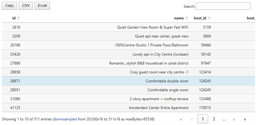
- This packages changes how Pandas and Polars DataFrames are rendered in Jupyter Notebooks. With
itablesyou can display your tables as interactive DataTables that you can sort, paginate, scroll or filter. - ITables is just about how tables are displayed. You can turn it on and off in just two lines, with no other impact on your data workflow.
Projects 1-2: Basic Statistical Data Analysis
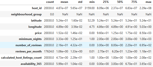
- Project 1:
ddf = pd.read_csv("listings.csv", index_col= "id")
print(ddf.shape)
(20030, 15)
print(ddf.columns)
Index(['name', 'host_id', 'host_name', 'neighbourhood_group', 'neighbourhood',
       'latitude', 'longitude', 'room_type', 'price', 'minimum_nights',
       'number_of_reviews', 'last_review', 'reviews_per_month',
       'calculated_host_listings_count', 'availability_365'],
      dtype='object')
ddf.describe().T
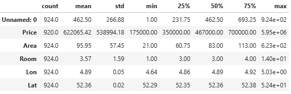
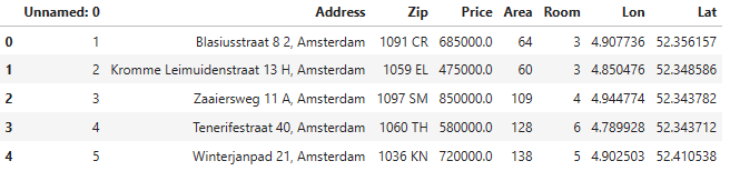
- Project 2:
ddf1 = pd.read_csv('HousingPrices-Amsterdam-August-2021.csv')
ddf1.head()
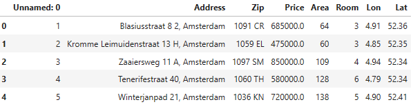
print(ddf1.shape)
(924, 8)
print(ddf1.columns)
Index(['Unnamed: 0', 'Address', 'Zip', 'Price', 'Area', 'Room', 'Lon', 'Lat'], dtype='object')
ddf1.describe().T
Projects 1-2: Exploratory Data Analysis (EDA) & ML
- Project 1
- Input data preparation
listings = pd.read_csv("listings.csv", index_col= "id")
target_columns = ["property_type", "accommodates", "first_review", "review_scores_value", "review_scores_cleanliness", "review_scores_location", "review_scores_accuracy", "review_scores_communication", "review_scores_checkin", "review_scores_rating", "maximum_nights", "listing_url", "host_is_superhost", "host_about", "host_response_time", "host_response_rate", "street", "weekly_price", "monthly_price", "market"]
listings = pd.merge(listings, listings_details[target_columns], on='id', how='left')
listings = listings.drop(columns=['neighbourhood_group'])
listings['host_response_rate'] = pd.to_numeric(listings['host_response_rate'].str.strip('%'))
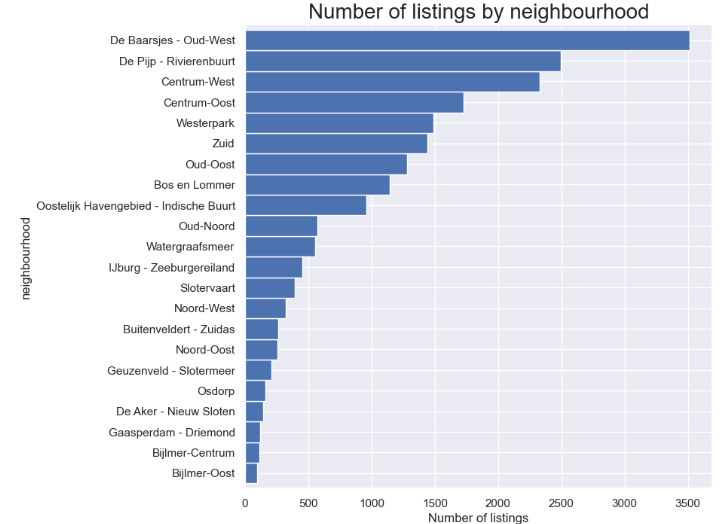
- Number of listings by neighborhood
feq=listings['neighbourhood'].value_counts().sort_values(ascending=True)
feq.plot.barh(figsize=(10, 8), color='b', width=1)
plt.title("Number of listings by neighbourhood", fontsize=20)
plt.xlabel('Number of listings', fontsize=12)
plt.show()
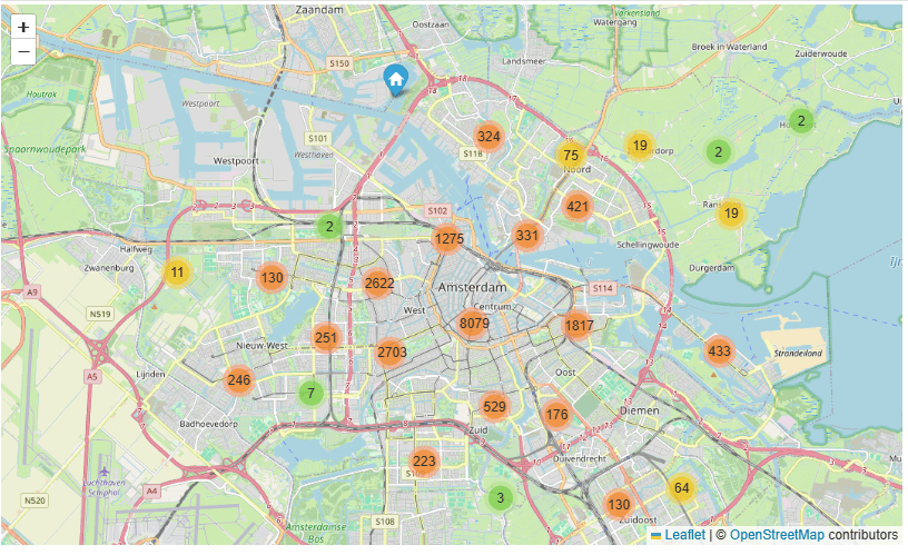
- AMS Open Street Location Map: number of listings per neighborhood
lats2018 = listings['latitude'].tolist()
lons2018 = listings['longitude'].tolist()
locations = list(zip(lats2018, lons2018))

map1 = folium.Map(location=[52.3680, 4.9036], zoom_start=11.5)
FastMarkerCluster(data=locations).add_to(map1)
map1
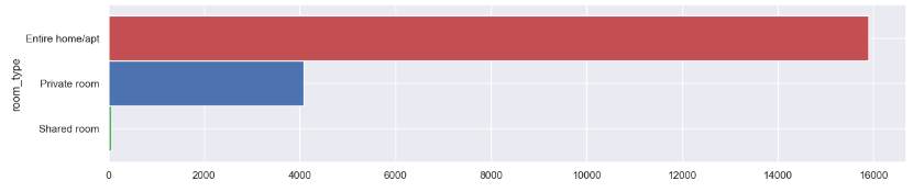
- Room type counts
freq = listings['room_type']. value_counts().sort_values(ascending=True)
freq.plot.barh(figsize=(15, 3), width=1, color = ["g","b","r"])
plt.show()
- Check unique property types in our listings
listings.property_type.unique()
array(['Apartment', 'Townhouse', 'Houseboat', 'Bed and breakfast', 'Boat',
       'Guest suite', 'Loft', 'Serviced apartment', 'House',
       'Boutique hotel', 'Guesthouse', 'Other', 'Condominium', 'Chalet',
       'Nature lodge', 'Tiny house', 'Hotel', 'Villa', 'Cabin',
       'Lighthouse', 'Bungalow', 'Hostel', 'Cottage', 'Tent',
       'Earth house', 'Campsite', 'Castle', 'Camper/RV', 'Barn',
       'Casa particular (Cuba)', 'Aparthotel'], dtype=object)
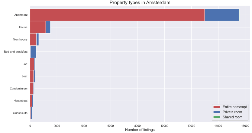
- Comparing property types in Amsterdam
prop = listings.groupby(['property_type','room_type']).room_type.count()
prop = prop.unstack()
prop['total'] = prop.iloc[:,0:3].sum(axis = 1)
prop = prop.sort_values(by=['total'])
prop = prop[prop['total']>=100]
prop = prop.drop(columns=['total'])

prop.plot(kind='barh',stacked=True, color = ["r","b","g"],
              linewidth = 1, grid=True, figsize=(15,8), width=1)
plt.title('Property types in Amsterdam', fontsize=18)
plt.xlabel('Number of listings', fontsize=14)
plt.ylabel("")
plt.legend(loc = 4,prop = {"size" : 13})
plt.rc('ytick', labelsize=13)
plt.show()
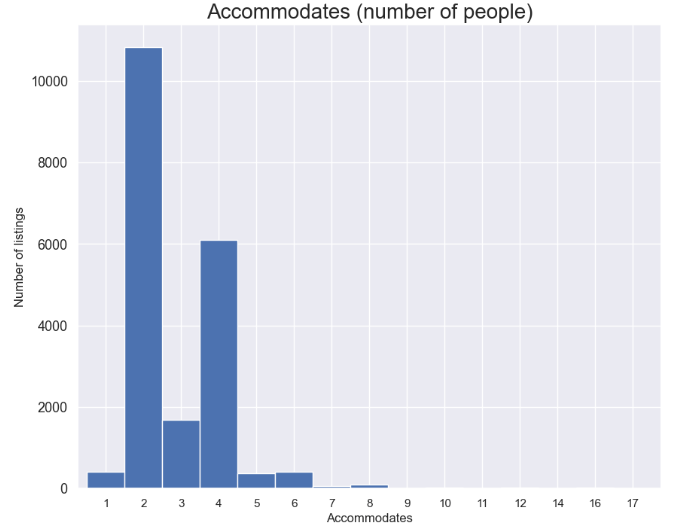
- Accommodates (number of people)
feq=listings['accommodates'].value_counts().sort_index()
feq.plot.bar(figsize=(10, 8), color='b', width=1, rot=0)
plt.title("Accommodates (number of people)", fontsize=20)
plt.ylabel('Number of listings', fontsize=12)
plt.xlabel('Accommodates', fontsize=12)
plt.show()
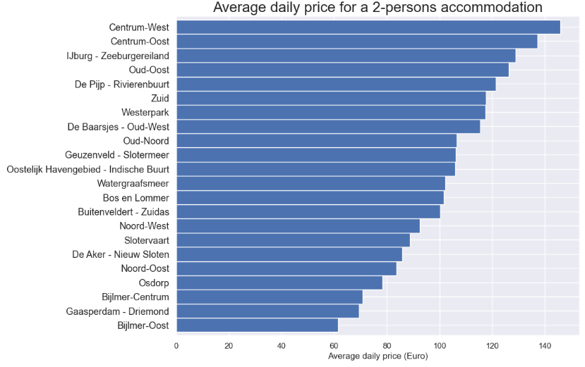
- Average daily price for a 2-persons accommodation
feq = listings[listings['accommodates']==2]
feq = feq.groupby('neighbourhood')['price'].mean().sort_values(ascending=True)
feq.plot.barh(figsize=(10, 8), color='b', width=1)
plt.title("Average daily price for a 2-persons accommodation", fontsize=20)
plt.xlabel('Average daily price (Euro)', fontsize=12)
plt.ylabel("")
plt.show()
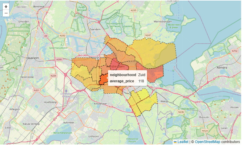
- City map average price per neighborhood
adam = gpd.read_file("neighbourhoods.geojson")
feq = pd.DataFrame([feq])
feq = feq.transpose()
adam = pd.merge(adam, feq, on='neighbourhood', how='left')
adam.rename(columns={'price': 'average_price'}, inplace=True)
adam.average_price = adam.average_price.round(decimals=0)

map_dict = adam.set_index('neighbourhood')['average_price'].to_dict()
color_scale = LinearColormap(['yellow','red'], vmin = min(map_dict.values()), vmax = max(map_dict.values()))

def get_color(feature):
    value = map_dict.get(feature['properties']['neighbourhood'])
    return color_scale(value)

map3 = folium.Map(location=[52.3680, 4.9036], zoom_start=11)
folium.GeoJson(data=adam,
               name='Amsterdam',
               tooltip=folium.features.GeoJsonTooltip(fields=['neighbourhood', 'average_price'],
                                                      labels=True,
                                                      sticky=False),
               style_function= lambda feature: {
                   'fillColor': get_color(feature),
                   'color': 'black',
                   'weight': 1,
                   'dashArray': '5, 5',
                   'fillOpacity':0.5
                   },
               highlight_function=lambda feature: {'weight':3, 'fillColor': get_color(feature), 'fillOpacity': 0.8}).add_to(map3)
map3
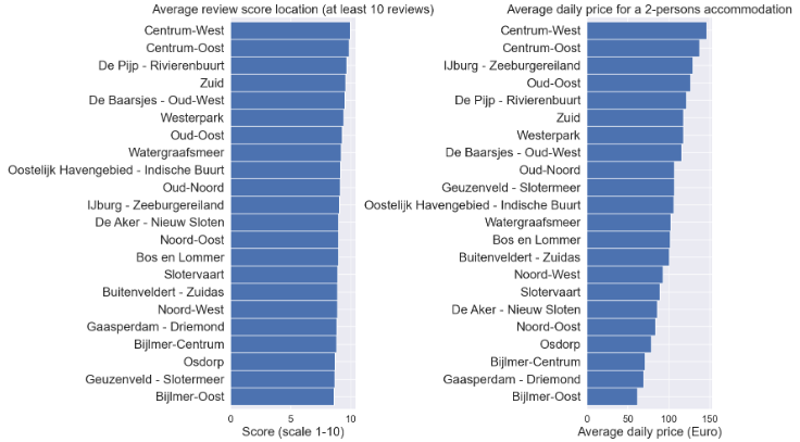
- Average review score location (at least 10 reviews) vs Average daily price for a 2-persons accommodation
fig = plt.figure(figsize=(20,10))
plt.rc('xtick', labelsize=16)
plt.rc('ytick', labelsize=20)

ax1 = fig.add_subplot(121)
feq = listings[listings['number_of_reviews']>=10]
feq1 = feq.groupby('neighbourhood')['review_scores_location'].mean().sort_values(ascending=True)
ax1=feq1.plot.barh(color='b', width=1)
plt.title("Average review score location (at least 10 reviews)", fontsize=20)
plt.xlabel('Score (scale 1-10)', fontsize=20)
plt.ylabel("")

ax2 = fig.add_subplot(122)
feq = listings[listings['accommodates']==2]
feq2 = feq.groupby('neighbourhood')['price'].mean().sort_values(ascending=True)
ax2=feq2.plot.barh(color='b', width=1)
plt.title("Average daily price for a 2-persons accommodation", fontsize=20)
plt.xlabel('Average daily price (Euro)', fontsize=20)
plt.ylabel("")

plt.tight_layout()
plt.show()
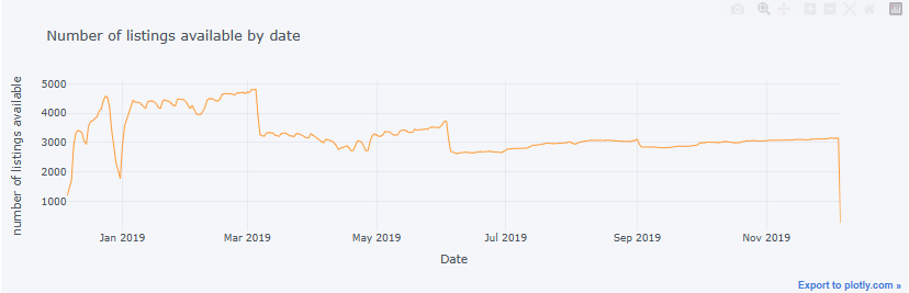
- Number of listings available by date
sum_available = calendar[calendar.available == "t"].groupby(['date']).size().to_frame(name= 'available').reset_index()
sum_available['weekday'] = sum_available['date'].dt.day_name()
sum_available = sum_available.set_index('date')

sum_available.iplot(y='available', mode = 'lines', xTitle = 'Date', yTitle = 'number of listings available',\
                   text='weekday', title = 'Number of listings available by date')
- Project 2
- Let’s consider the Amsterdam House Price Prediction project, including data processing, EDA, feature engineering, and ML regression. Read more here.
- Basic imports and reading the input dataset
import numpy as np # linear algebra
import pandas as pd # data processing, CSV file I/O (e.g. pd.read_csv)
import warnings
warnings.filterwarnings('ignore')
import matplotlib.pyplot as plt
import seaborn as sns
from sklearn.model_selection import cross_val_score
from sklearn.metrics import mean_squared_error
df = pd.read_csv('HousingPrices-Amsterdam-August-2021.csv')
df.head()
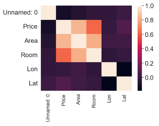
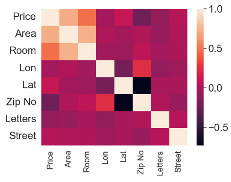
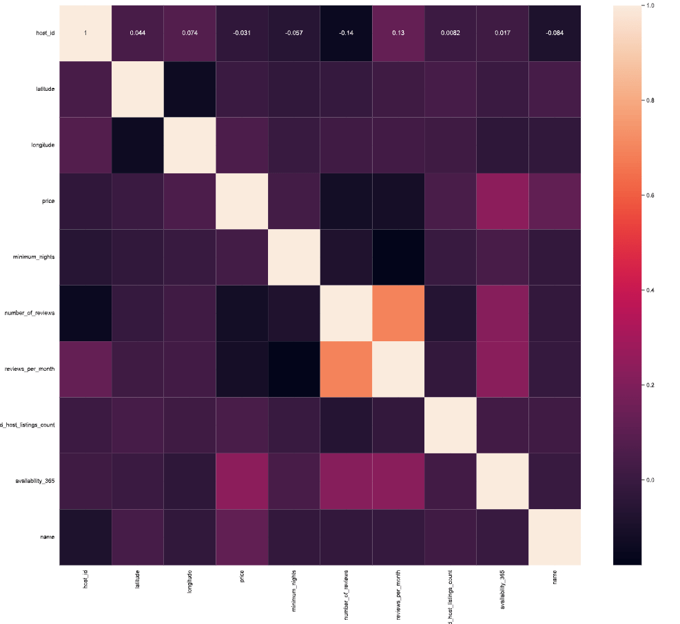
- Plotting the feature correlation heatmap
sns.heatmap(df.corr())
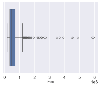
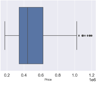
- Removing undefined values while examining the price outliers with boxplots
df = df.dropna(axis = 0, inplace = False)
sns.boxplot(x='Price', data = df)
- Removing price outliers with the IQR thresholds
q1 = df.describe()['Price']['25%']
q3 = df.describe()['Price']['75%']
iqr = q3 - q1
max_price = q3 + 1.5 * iqr
outliers = df[df['Price'] >= max_price]
outliers_count = outliers['Price'].count()
df_count = df['Price'].count()
print('Percentage removed: ' + str(round(outliers_count/df_count * 100, 2)) + '%')
Percentage removed: 7.72%
df= df[df['Price'] <= max_price]
sns.boxplot(x='Price', data = df)
- Input data editing and plotting the modified feature correlation heatmap
df['Zip No'] = df['Zip'].apply(lambda x:x.split()[0])
df['Letters'] = df['Zip'].apply(lambda x:x.split()[-1])
def word_separator(string):
    list = string.split()
    word = []
    number = []
    for element in list:
        if element.isalpha() == True:
            word.append(element)
        else:
            break
    word = ' '.join(word)
    return word
df['Street'] = df['Address'].apply(lambda x:word_separator(x))
numerical = ['Price', 'Area', 'Room', 'Lon', 'Lat']
categorical = ['Address', 'Zip No', 'Letters', 'Street']
from sklearn.preprocessing import LabelEncoder
for c in categorical:
    lbl = LabelEncoder()
    lbl.fit(list(df[c].values))
    df[c] = lbl.transform(list(df[c].values))
df.drop(['Zip', 'Unnamed: 0', 'Address'], axis =1, inplace = True)
sns.heatmap(df.corr())
- Preparing data for training and testing supervised ML models
from sklearn.model_selection import train_test_split
X = df.drop('Price', axis =1)
y = df['Price']
X_train, X_test, y_train, y_test = train_test_split(X,y, test_size = 0.4)
from sklearn.preprocessing import StandardScaler
scaler = StandardScaler()
X_train = scaler.fit_transform(X_train)
X_test = scaler.transform(X_test)
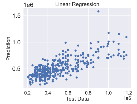
- Linear Regression (LR)
from sklearn.linear_model import LinearRegression
linreg = LinearRegression()
linreg.fit(X_train, y_train)
predictions = linreg.predict(X_test)
plt.scatter(y_test,predictions)
plt.title('Linear Regression',fontsize=18)
plt.xlabel('Test Data',fontsize=18)
plt.ylabel('Prediction',fontsize=18)
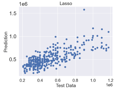
- Lasso regression
from sklearn.linear_model import Lasso
lasso = Lasso()
lasso.fit(X_train, y_train)
predictions = lasso.predict(X_test)
plt.scatter(y_test,predictions)
plt.title('Lasso',fontsize=18)
plt.xlabel('Test Data',fontsize=18)
plt.ylabel('Prediction',fontsize=18)
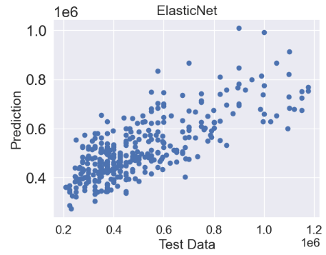
- ElasticNet regression
from sklearn.linear_model import ElasticNet
elasticnet = ElasticNet()
elasticnet.fit(X_train, y_train)
predictions = elasticnet.predict(X_test)
plt.scatter(y_test,predictions)
plt.title('ElasticNet',fontsize=18)
plt.xlabel('Test Data',fontsize=18)
plt.ylabel('Prediction',fontsize=18)
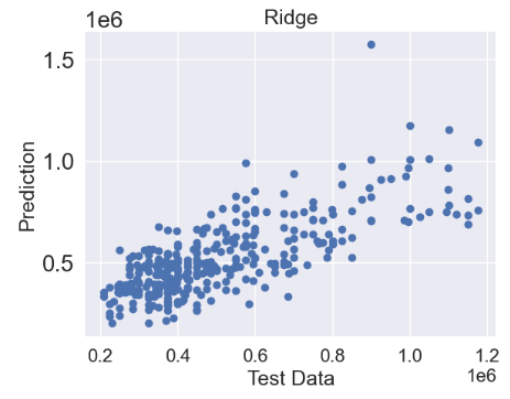
- Ridge regression
from sklearn.linear_model import Ridge
ridge = Ridge()
ridge.fit(X_train, y_train)
predictions = ridge.predict(X_test)
plt.scatter(y_test,predictions)
plt.title('Ridge',fontsize=18)
plt.xlabel('Test Data',fontsize=18)
plt.ylabel('Prediction',fontsize=18)
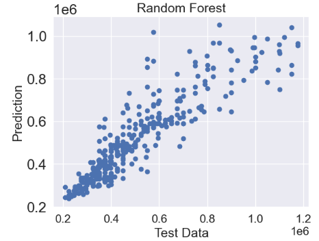
- Random Forest (RF) Regressor
from sklearn.ensemble import RandomForestRegressor
random_forest = RandomForestRegressor()
random_forest.fit(X_train, y_train)
predictions = random_forest.predict(X_test)
plt.scatter(y_test,predictions)
plt.title('Random Forest',fontsize=18)
plt.xlabel('Test Data',fontsize=18)
plt.ylabel('Prediction',fontsize=18)
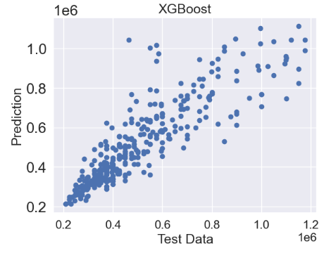
- XGBoost Regressor
from xgboost import XGBRegressor
xgb = XGBRegressor()
xgb.fit(X_train, y_train)
predictions = xgb.predict(X_test)
plt.scatter(y_test,predictions)
plt.title('XGBoost',fontsize=18)
plt.xlabel('Test Data',fontsize=18)
plt.ylabel('Prediction',fontsize=18)
- Random Forest Hyperparameter Optimization (HPO)
from sklearn.model_selection import RandomizedSearchCV, GridSearchCV

random_grid = {'bootstrap': [True, False],
 'max_depth': [10, 20, 30, 40, 50, 60, 70, 80, 90, 100, None],
 'max_features': ['auto', 'sqrt'],
 'min_samples_leaf': [1, 2, 4],
 'min_samples_split': [2, 5, 10],
 'n_estimators': [200, 400, 600, 800, 1000, 1200, 1400, 1600, 1800, 2000]}

random_cv = RandomizedSearchCV(estimator = random_forest, param_distributions = random_grid, n_iter = 100, cv = 10, verbose = 2, n_jobs = -1)
random_cv.fit(X_train, y_train)
Fitting 10 folds for each of 100 candidates, totalling 1000 fits
RandomizedSearchCV(cv=10, estimator=RandomForestRegressor(), n_iter=100,
                   n_jobs=-1,
                   param_distributions={'bootstrap': [True, False],
                                        'max_depth': [10, 20, 30, 40, 50, 60,
                                                      70, 80, 90, 100, None],
                                        'max_features': ['auto', 'sqrt'],
                                        'min_samples_leaf': [1, 2, 4],
                                        'min_samples_split': [2, 5, 10],
                                        'n_estimators': [200, 400, 600, 800,
                                                         1000, 1200, 1400, 1600,
                                                         1800, 2000]},
                   verbose=2)
random_cv.best_params_
{'n_estimators': 1400,
 'min_samples_split': 2,
 'min_samples_leaf': 2,
 'max_features': 'sqrt',
 'max_depth': 100,
 'bootstrap': False}

param_grid = {'bootstrap': [True, False],
'max_depth': [60,65,70,75,80],
'min_samples_leaf':[1,2,3],
'min_samples_split': [1,2,3],
'n_estimators': [1750,1760,1770,1780,1790,1800,1810,1820,1830,1840,1850]}
grid_search = GridSearchCV(estimator = random_forest, param_grid = param_grid, cv = 3, n_jobs = -1, verbose = 2)

grid_search.fit(X_train,y_train)

Fitting 3 folds for each of 990 candidates, totalling 2970 fits
GridSearchCV(cv=3, estimator=RandomForestRegressor(), n_jobs=-1,
             param_grid={'bootstrap': [True, False],
                         'max_depth': [60, 65, 70, 75, 80],
                         'min_samples_leaf': [1, 2, 3],
                         'min_samples_split': [1, 2, 3],
                         'n_estimators': [1750, 1760, 1770, 1780, 1790, 1800,
                                          1810, 1820, 1830, 1840, 1850]},
             verbose=2)

grid_search.best_params_
{'bootstrap': True,
 'max_depth': 65,
 'min_samples_leaf': 1,
 'min_samples_split': 2,
 'n_estimators': 1840}
tuned_random_forest = RandomForestRegressor(n_estimators = 1750, max_depth = 80, min_samples_leaf = 1, min_samples_split = 2)
random_forest.fit(X_train, y_train)
predictions = random_forest.predict(X_test)

cv = cross_val_score(tuned_random_forest, X_train, y_train, cv=20, scoring = 'neg_mean_squared_error')
print("The Random Forest Regressor with tuned parameters has a RMSE of: " + str(abs(cv.mean())**0.5))
The Random Forest Regressor with tuned parameters has a RMSE of: 95830.77429927936
# Calculate testing scores
from sklearn.metrics import mean_absolute_error, r2_score
test_mae = mean_absolute_error(y_test, predictions)
test_mse = mean_squared_error(y_test, predictions)
test_rmse = mean_squared_error(y_test, predictions, squared=False)
test_r2 = r2_score(y_test, predictions)
print(test_mae)
65426.81317647059
print(test_mse)
9152415095.08142
print(test_rmse)
95668.25541986966
print(test_r2)
0.8319334007165564
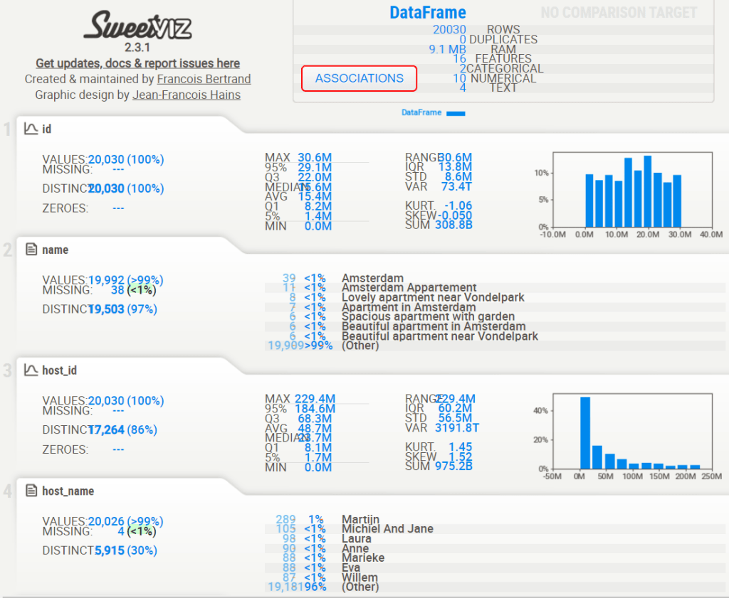
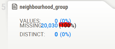
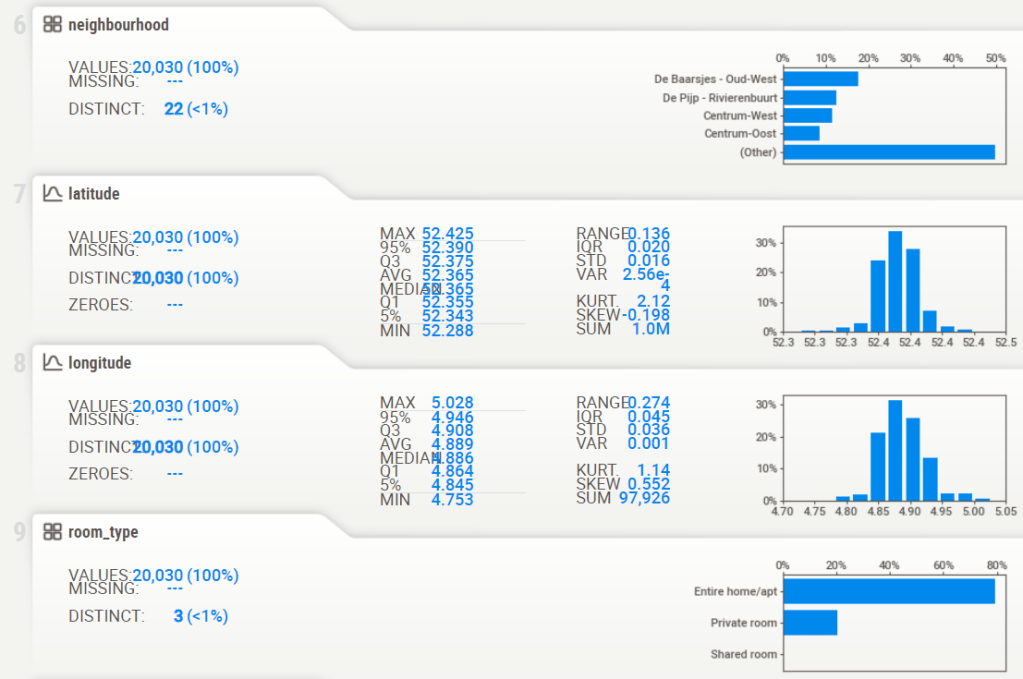
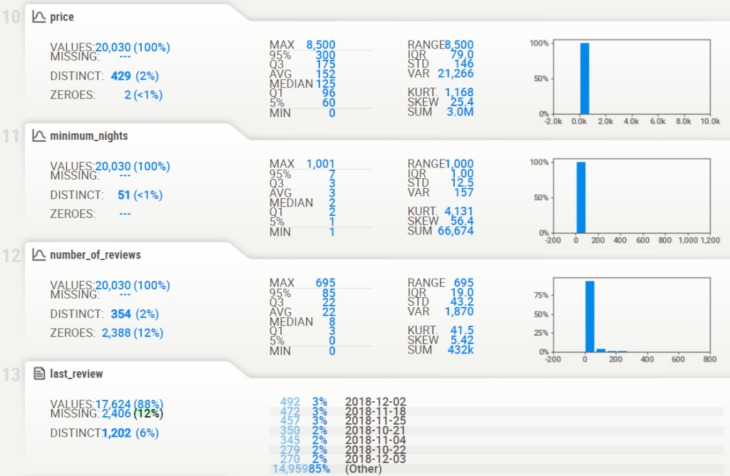
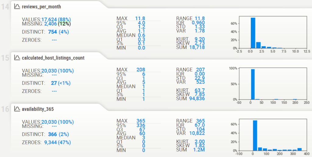
Project 1: SweetViz AutoEDA
- Project 1: Reading input data & displaying the sweetviz EDA HTML report
listings = pd.read_csv('listings.csv')
# importing sweetviz
import sweetviz as sv
#analyzing the dataset
advert_report = sv.analyze(listings)
#display the report
advert_report.show_html('listings_sv.html')
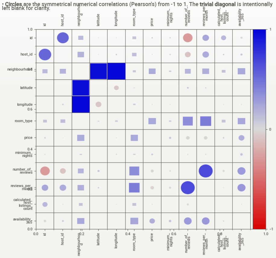
- Associations [Only including dataset “DataFrame”]
- ■ Squares are categorical associations (uncertainty coefficient & correlation ratio) from 0 to 1. The uncertainty coefficient is asymmetrical, (i.e. ROW LABEL values indicate how much they PROVIDE INFORMATION to each LABEL at the TOP).
- Circles are the symmetrical numerical correlations (Pearson’s) from -1 to 1. The trivial diagonal is intentionally left blank for clarity.
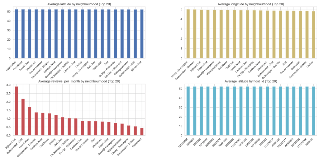
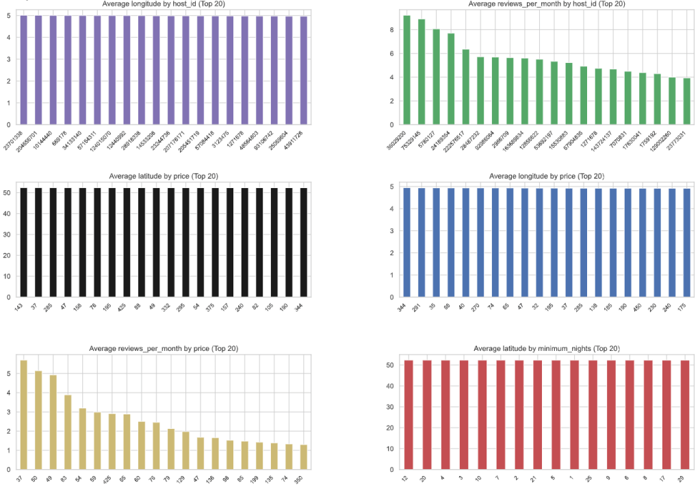
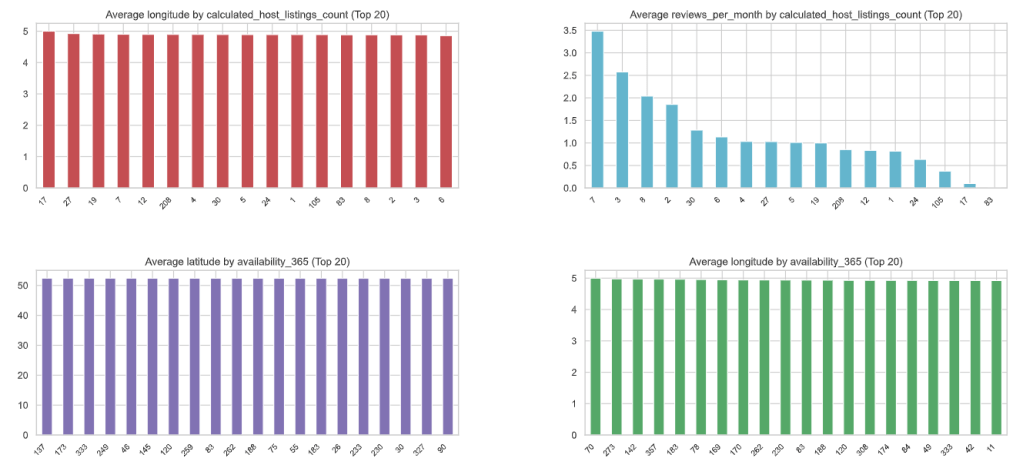
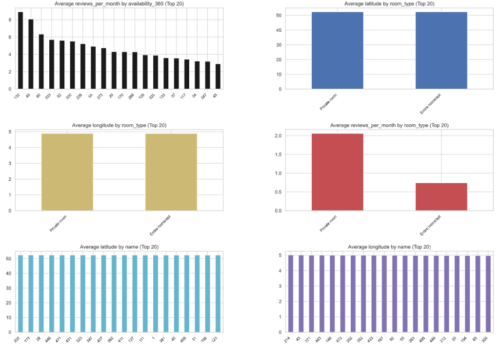
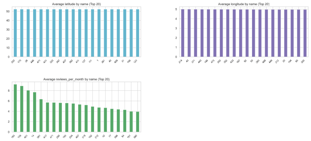
Project 1: AutoViz AutoEDA
- Project 1: Let’s explore the AutoViz EDA library. With just one line of code, you can effortlessly generate multiple informative plots, while addressing Data Quality issues.
- Defining the input csv file and loading the AutoViz Class
filename = "listings.csv"
target_variable = "name"
#Load Autoviz
from autoviz import AutoViz_Class
%matplotlib inline

AV = AutoViz_Class()
dft = AV.AutoViz(
    filename,
    sep=",",
    depVar=target_variable,
    dfte=None,
    header=0,
    verbose=2,
    lowess=False,
    chart_format="svg",
    max_rows_analyzed=500,
    max_cols_analyzed=20,
    save_plot_dir=None
)
from autoviz import FixDQ
fixdq = FixDQ()
- AutoViz Log Output
max_rows_analyzed is smaller than dataset shape 20030...
randomly sampled 500 rows from read CSV file
Shape of your Data Set loaded: (500, 16)
#######################################################################################
######################## C L A S S I F Y I N G V A R I A B L E S ####################
#######################################################################################
Classifying variables in data set...
Printing upto 30 columns (max) in each category:
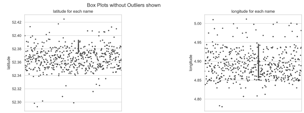
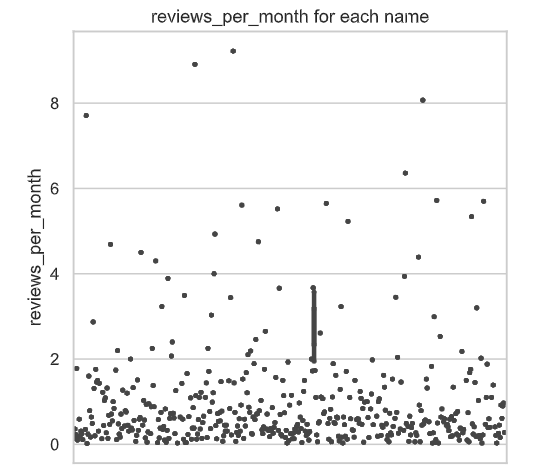
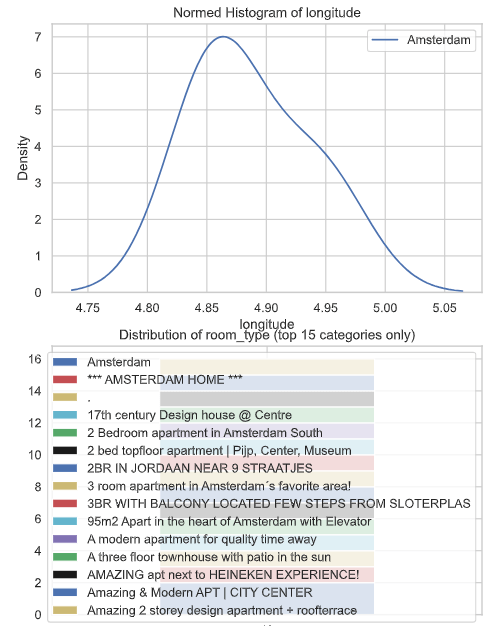
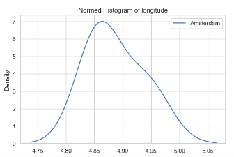
Numeric Columns : ['latitude', 'longitude', 'reviews_per_month']
Integer-Categorical Columns: ['host_id', 'price', 'minimum_nights', 'number_of_reviews', 'calculated_host_listings_count', 'availability_365']
String-Categorical Columns: ['neighbourhood']
Factor-Categorical Columns: []
String-Boolean Columns: ['room_type']
Numeric-Boolean Columns: []
Discrete String Columns: ['host_name', 'last_review']
NLP text Columns: []
Date Time Columns: []
ID Columns: ['id']
Columns that will not be considered in modeling: ['neighbourhood_group']
15 Predictors classified...
2 variable(s) removed since they were ID or low-information variables
List of variables removed: ['id', 'neighbourhood_group']
Since Number of Rows in data 500 exceeds maximum, randomly sampling 500 rows for EDA...
################ Multi_Classification problem #####################
Columns to delete:
" ['neighbourhood_group']"
Boolean variables %s
" ['room_type']"
Categorical variables %s
(" ['neighbourhood', 'host_id', 'price', 'minimum_nights', "
"'number_of_reviews', 'calculated_host_listings_count', 'availability_365', "
"'room_type']")
Continuous variables %s
" ['latitude', 'longitude', 'reviews_per_month']"
Discrete string variables %s
" ['host_name', 'last_review']"
Date and time variables %s
' []'
ID variables %s
" ['id']"
Target variable %s
' name'
To fix these data quality issues in the dataset, import FixDQ from autoviz...
All variables classified into correct types.
- AutoViz HTML Plots in the new sub-directory name:
- Bar Plots
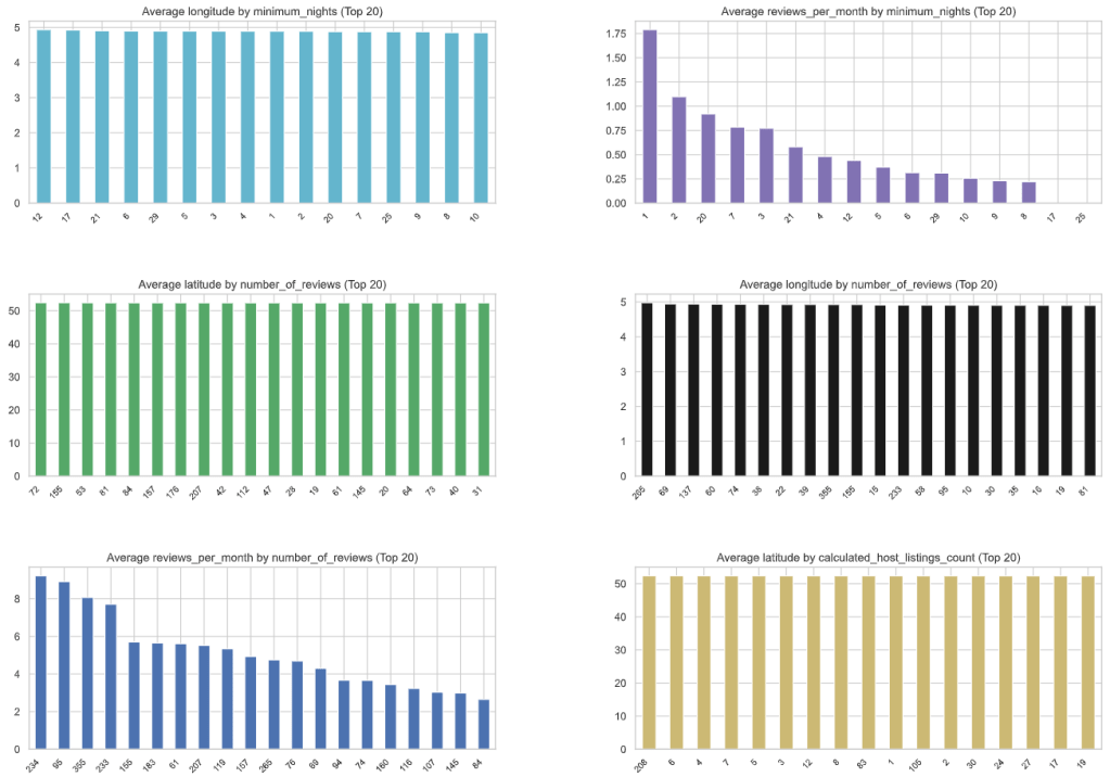
- Box Plots
- Dist Plots Numerics
- Heat Map
Project 1: Geospatial EDA
- Let’s follow the Plotly Geospatial EDA.
- Basic imports and downloads
import numpy as np
import pandas as pd
import seaborn as sns
sns.set()
import matplotlib.pyplot as plt

import os
import warnings
warnings.simplefilter(action='ignore', category=FutureWarning)

#to make the interactive maps
import folium
from folium.plugins import FastMarkerCluster
import geopandas as gpd
from branca.colormap import LinearColormap

#to make the plotly graphs
import plotly.graph_objs as go
import chart_studio.plotly as py
from plotly.offline import iplot, init_notebook_mode
import cufflinks
cufflinks.go_offline(connected=True)
init_notebook_mode(connected=True)

#text mining
from nltk.tokenize import word_tokenize
from nltk.corpus import stopwords
import re
from sklearn.feature_extraction.text import TfidfVectorizer, CountVectorizer
from wordcloud import WordCloud
from json.decoder import JSONDecoder
import warnings


warnings.simplefilter(action='ignore', category=FutureWarning)


import numpy as np
import pandas as pd
import plotly.express as px
import plotly.io as pio
import nltk
from nltk.corpus import stopwords
from nltk.tokenize import word_tokenize
from nltk.stem import WordNetLemmatizer
from wordcloud import WordCloud


nltk.download('punkt', quiet=True)
nltk.download('wordnet', quiet=True)
nltk.download('stopwords', quiet=True)
nltk.download('omw-1.4', quiet=True)

lemmatizer = WordNetLemmatizer()
stop_words = set(stopwords.words('english') + ['ha', 'wa', 'br', 'b'])
- Preprocessing and plotting functions
def preprocess(text):
    text = list(filter(str.isalpha, word_tokenize(text)))
    text = list(lemmatizer.lemmatize(word) for word in text)
    text = list(word for word in text if word not in stop_words)
    return ' '.join(text)


def draw_wordcloud(texts, max_words=1000, width=1000, height=500):
    wordcloud = WordCloud(background_color='white', max_words=max_words,
                          width=width, height=height)
    joint_texts = ' '.join(list(texts))
    wordcloud.generate(joint_texts)
    return wordcloud.to_image()


def draw_choropleth(neighbourhoods_geojson,feature, stat='mean', only_reviewed=False, title=None):
    stats = {
        'mean': pd.api.typing.DataFrameGroupBy.mean,
        'median': pd.api.typing.DataFrameGroupBy.median,
        'sum': pd.api.typing.DataFrameGroupBy.sum,
    }
    gb = stats[stat]((listings_reviewed if only_reviewed else listings).groupby(by='neighbourhood', as_index=False), feature)
    fig = px.choropleth_mapbox(gb, geojson=neighbourhoods_geojson, color=feature,
                           locations="neighbourhood", featureidkey="properties.neighbourhood",
                           center={"lat": 52.3676, "lon": 4.9041}, title=title or f'{feature} by neighbourhood',
                           mapbox_style="carto-positron", zoom=10, opacity=0.5)
    return fig.show()
- Reading and preparing the input data of Project 1
calendar = pd.read_csv('calendar.csv')
listings = pd.read_csv('listings.csv')
listings_detailed = pd.read_csv('listings_details.csv')
reviews = pd.read_csv('reviews.csv')
reviews_detailed = pd.read_csv('reviews_details.csv')
neighbourhoods = pd.read_csv('neighbourhoods.csv')
listings = listings_detailed.drop(columns=['neighbourhood']).rename(columns={'neighbourhood_cleansed': 'neighbourhood'})  # we will only need neighbourhood_cleansed
reviews = reviews_detailed
for column in ['host_since', 'first_review', 'last_review']:
    listings[column] = pd.to_datetime(listings[column], format='%Y-%m-%d')
    listings[column].dt.day.describe()

calendar.date = pd.to_datetime(calendar.date, format='%Y-%m-%d')

listings.price = listings.price.replace('[\$,]', '', regex=True).astype(float)
calendar.price = calendar.price.replace('[\$,]', '', regex=True).astype(float)
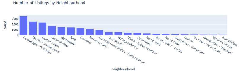
- Bar plot Number of Listings by Neighborhood
fig = px.histogram(listings, x="neighbourhood", category_orders={'neighbourhood': list(listings.neighbourhood.value_counts().index)}, title='Number of Listings by Neighbourhood')
fig.show()
- Preparing data for geospatial mapping
adam = gpd.read_file("neighbourhoods.geojson")
adam.head()
neighbourhood	neighbourhood_group	geometry
0	Bijlmer-Oost	None	MULTIPOLYGON Z (((4.99167 52.32444 43.06929, 4...
1	Noord-Oost	None	MULTIPOLYGON Z (((5.07916 52.38865 42.95663, 5...
2	Noord-West	None	MULTIPOLYGON Z (((4.93072 52.41161 42.91539, 4...
3	Oud-Noord	None	MULTIPOLYGON Z (((4.95242 52.38983 42.95411, 4...
4	IJburg - Zeeburgereiland	None	MULTIPOLYGON Z (((5.03906 52.35458 43.01664, 5...
gb = listings.neighbourhood.value_counts().reset_index()
gb.head()
index	neighbourhood
0	De Baarsjes - Oud-West	3515
1	De Pijp - Rivierenbuurt	2493
2	Centrum-West	2326
3	Centrum-Oost	1730
4	Westerpark	1490
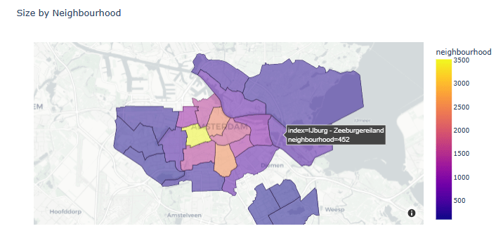
- Plotting Size by Neighborhood
gb = listings.neighbourhood.value_counts().reset_index()
fig = px.choropleth_mapbox(gb, geojson=adam, color='neighbourhood',
                       locations="index", featureidkey="properties.neighbourhood",
                       center={"lat": 52.3676, "lon": 4.9041}, title=f'Size by Neighbourhood',
                       mapbox_style="carto-positron", zoom=10, opacity=0.5)
fig.show()
- Printing top 10 neighborhoods
top10_neighbourhoods = list(listings.neighbourhood.value_counts()[:10].index)
top10_neighbourhoods
['De Baarsjes - Oud-West',
 'De Pijp - Rivierenbuurt',
 'Centrum-West',
 'Centrum-Oost',
 'Westerpark',
 'Zuid',
 'Oud-Oost',
 'Bos en Lommer',
 'Oostelijk Havengebied - Indische Buurt',
 'Oud-Noord']
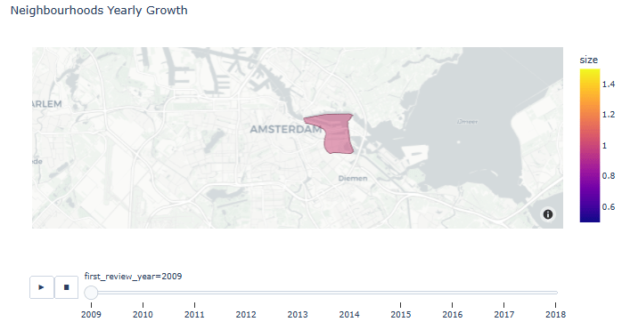
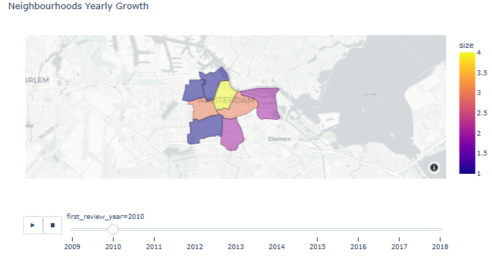
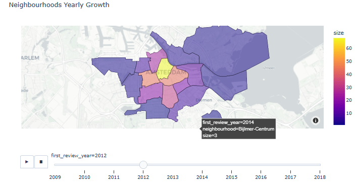
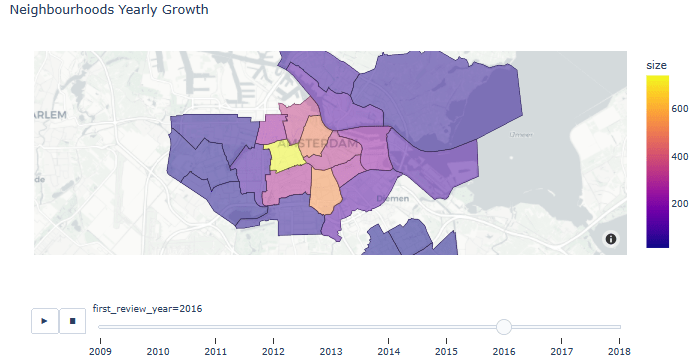
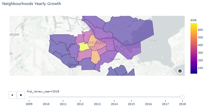
- Animated Neighborhoods Yearly Growth
listings_reviewed = listings[listings.number_of_reviews > 0]
listings_reviewed.loc[:, 'first_review_year'] = listings_reviewed['first_review'].dt.year
gb = listings_reviewed.groupby(by=['first_review_year', 'neighbourhood'], as_index=False).size()
gb.first_review_year = gb.first_review_year.astype(int)
fig = px.choropleth_mapbox(gb, geojson=adam, color='size',
                       locations="neighbourhood", featureidkey="properties.neighbourhood",
                       center={"lat": 52.3676, "lon": 4.9041}, title='Neighbourhoods Yearly Growth',
                       mapbox_style="carto-positron", zoom=10, opacity=0.5, animation_frame='first_review_year')
fig.show()
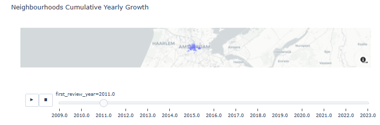
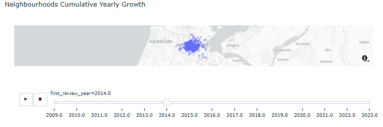
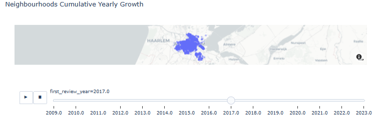
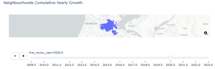
- Neighborhoods Cumulative Yearly Growth
res = listings_reviewed.copy()
for year in range(2009, 2023):
    listings_at_year = listings_reviewed[listings_reviewed.first_review_year == year]
    ls = [res]
    for future_year in range(year + 1, 2024):
        l = listings_at_year.copy()
        l.first_review_year = future_year
        ls.append(l)
    res = pd.concat(ls)
fig = px.scatter_mapbox(res.sort_values('first_review_year', ascending=True), lat='latitude', lon='longitude', center={"lat": 52.3676, "lon": 4.9041}, #color="peak_hour", size="car_hours",
                        zoom=10, mapbox_style="carto-positron", animation_frame='first_review_year', opacity=0.25, title='Neighbourhoods Cumulative Yearly Growth')
fig.show()
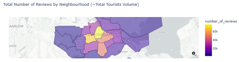
- Total Number of Reviews by Neighborhood (~Total Tourists Volume)
draw_choropleth(adam,'number_of_reviews', 'sum', title='Total Number of Reviews by Neighbourhood (~Total Tourists Volume)')
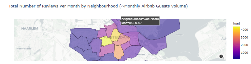
- Total Number of Reviews Per Month by Neighborhood (~Monthly Airbnb Guests Volume)
listings_reviewed['lifetime_in_months'] = ((listings_reviewed.last_review - listings_reviewed.first_review)/np.timedelta64(1, 'D'))/30 + 1/30
listings_reviewed['load'] = listings_reviewed['number_of_reviews'] / np.ceil(listings_reviewed['lifetime_in_months']
draw_choropleth(adam,'load', 'sum', only_reviewed=True, title='Total Number of Reviews Per Month by Neighbourhood (~Monthly Airbnb Guests Volume)')
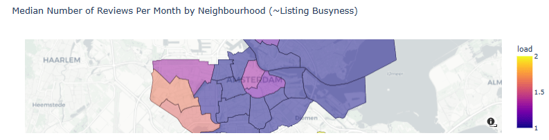
- Median Number of Reviews Per Month by Neighborhood (~Listing Busyness)
draw_choropleth(adam,'load', 'median', only_reviewed=True, title='Median Number of Reviews Per Month by Neighbourhood (~Listing Busyness)')
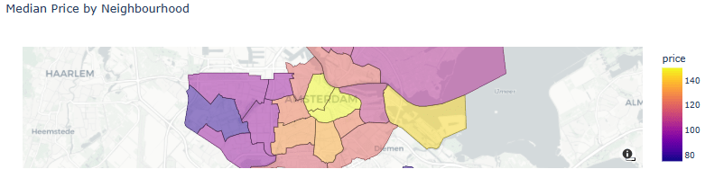
- Median Price by Neighborhood
draw_choropleth(adam,'price', 'median', title='Median Price by Neighbourhood')
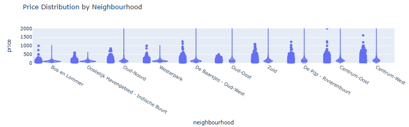
- Violin Plot of Price Distribution by Neighborhood (top 10 areas)
listings_in_top10_neighbourhoods = listings[listings.neighbourhood.isin(top10_neighbourhoods)]
len(listings_in_top10_neighbourhoods)
16952
fig = px.violin(listings_in_top10_neighbourhoods, y="price", x="neighbourhood", log_y=False, range_y=[-10, 2000], points="all", box=True, title='Price Distribution by Neighbourhood',
               category_orders={'neighbourhood': list(listings_in_top10_neighbourhoods.groupby('neighbourhood')['price'].aggregate('median').reset_index().sort_values(by='price')['neighbourhood'])}
)
fig.show()
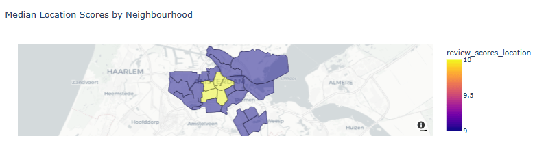
- Median Location Scores by Neighborhood
draw_choropleth(adam,'review_scores_location', 'median', title='Median Location Scores by Neighbourhood')
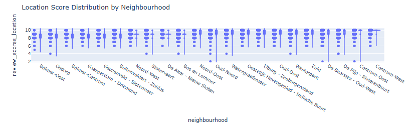
- Violin Plot of Location Score Distribution by Neighborhood
fig = px.violin(listings, y="review_scores_location", x="neighbourhood", box=True, points="all", range_y=[1.8, 10.5], title='Location Score Distribution by Neighbourhood',
               category_orders={'neighbourhood': list(listings.groupby('neighbourhood')['review_scores_location'].aggregate('mean').reset_index().sort_values(by='review_scores_location')['neighbourhood'])}
)
fig.show()
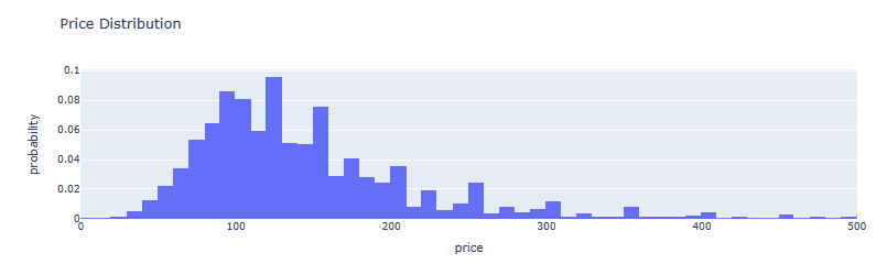
- AMS Price Distribution histogram
fig = px.histogram(listings, x='price', nbins=1000, barmode='group', range_x=[0, 500], histnorm='probability', title='Price Distribution')
fig.show()
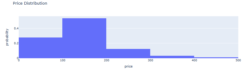
- AMS Price-to-Probability Distribution histogram
fig = px.histogram(listings, x='price', nbins=100, barmode='group', range_x=[0, 500], histnorm='probability', title='Price Distribution')
fig.show()
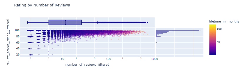
- Rating by Number of Reviews scatter plot
listings_reviewed.loc[:, 'number_of_reviews_jittered'] = listings_reviewed.number_of_reviews + np.exp(np.random.randn(len(listings_reviewed)) / 10)
listings_reviewed.loc[:, 'review_scores_rating_jittered'] = listings_reviewed.review_scores_rating + np.random.randn(len(listings_reviewed)) / 10
fig = px.scatter(listings_reviewed[listings_reviewed.price < 1000], x='number_of_reviews_jittered', y='review_scores_rating_jittered', color='lifetime_in_months', log_x=True, opacity=0.25, marginal_x='box', marginal_y='histogram', title='Rating by Number of Reviews')
fig.show()
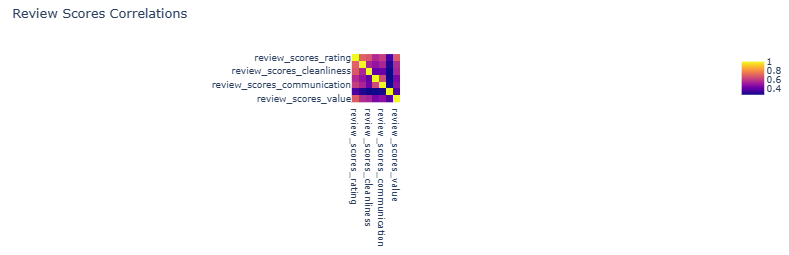
- Review Scores Correlations heatmap
aspect_scores_feats = ['review_scores_accuracy', 'review_scores_cleanliness', 'review_scores_checkin', 'review_scores_communication', 'review_scores_location', 'review_scores_value']
scores_feats = ['review_scores_rating'] + aspect_scores_feats
px.imshow(listings[scores_feats].corr(), title='Review Scores Correlations')
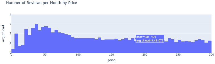
- Number of Reviews per Month by Price
listings_reviewed.loc[:, 'load_jittered'] = listings_reviewed.load + np.random.randn(len(listings_reviewed)) / 5
listings_reviewed.loc[:, 'price_jittered'] = listings_reviewed.price + np.random.randn(len(listings_reviewed)) * 2

px.histogram(listings_reviewed, x='price', y='load', histfunc='avg', range_x=[0, 300], range_y=[0, 4], nbins=2500, title='Number of Reviews per Month by Price').show()
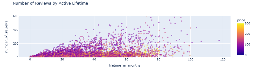
- Number of Reviews by Active Lifetime scatter plot
px.scatter(listings_reviewed, x='lifetime_in_months', y='number_of_reviews', color='price', range_color=[0, 300], range_y=[0, 600], opacity=0.5, title='Number of Reviews by Active Lifetime').show()
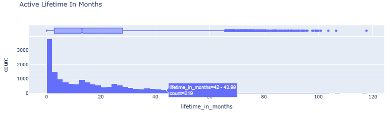
- Active Lifetime In Months histogram vs boxplot
fig = px.histogram(listings_reviewed, x='lifetime_in_months', nbins=int(listings_reviewed.lifetime_in_months.max()), barmode='group', marginal='box', title='Active Lifetime In Months')
fig.show()
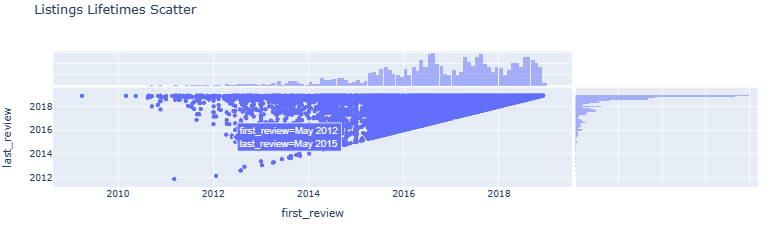
- Listings Lifetimes Scatter
fig = px.scatter(listings, x='first_review', y='last_review', marginal_x='histogram', marginal_y='histogram', title='Listings Lifetimes Scatter')
fig.show()
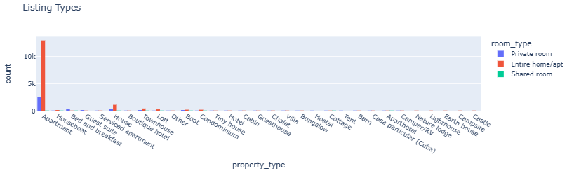
- Listing Types
fig = px.histogram(listings, x='property_type', color='room_type', barmode='group', title='Listing Types')
fig.show()
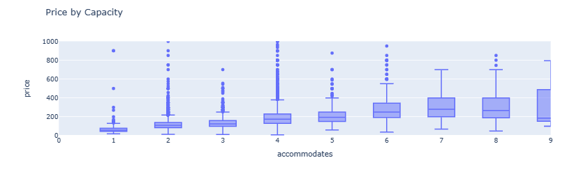
- Price by Capacity boxplots
fig = px.box(listings, x='accommodates', y='price', range_y=[0, 1000], range_x=[0, 9], title='Price by Capacity')
fig.show()
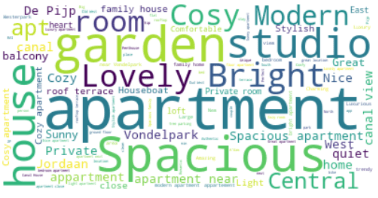
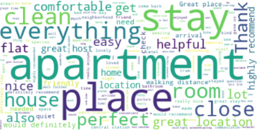
Project 1: NLP Wordcloud Images
- Let’s generate a word cloud image of the aforementioned listings.
- Preparing the input text data
listings['listing_name'] = listings.name.astype('string')
print(listings['listing_name'])
0                 Quiet Garden View Room & Super Fast WiFi
1                        Quiet apt near center, great view
2               100%Centre-Studio 1 Private Floor/Bathroom
3                      Lovely apt in City Centre (Jordaan)
4        Romantic, stylish B&B houseboat in canal district
                               ...
20025     Family House City + free Parking+garden (160 m2)
20026                    Home Sweet Home in Indische Buurt
20027               Amsterdam Cozy apartment nearby center
20028              Home Sweet Home for a Guest or a Couple
20029          Cosy two bedroom appartment near 'de Pijp'!
Name: listing_name, Length: 20000, dtype: string
txt=listings['listing_name'].str.cat(sep=' ')
- Creating and generating the word cloud
# Create and generate a word cloud image:

wordcloud = WordCloud().generate(txt)
type(txt)
str
# Display the generated image:
plt.imshow(wordcloud, interpolation='bilinear')
plt.axis("off")
plt.show()

- Using stop words
STOPWORDS = nltk.corpus.stopwords.words('english')
# Create stopword list:
stopwords = set(STOPWORDS)
stopwords.update(["Amsterdam", "city", "Beautiful","centre",'center'])

# Generate a word cloud image
wordcloud = WordCloud(stopwords=stopwords, background_color="white").generate(txt)

# Display the generated image:
# the matplotlib way:
plt.imshow(wordcloud, interpolation='bilinear')
plt.axis("off")
plt.show()
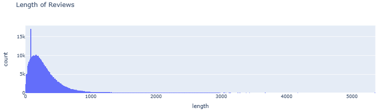
- Examining the Length of Reviews
reviews = reviews.dropna()
reviews.loc[:, 'length'] = reviews.comments.str.len()
fig = px.histogram(reviews[reviews.length != 0], x='length', nbins=1000, barmode='group', title='Length of Reviews')
fig.show()
- Restricting the Length of Reviews by 750
reviews = reviews[reviews.length < 750]
reviews_with_rating = reviews.join(listings[['id', 'review_scores_rating']].set_index('id'), on='listing_id', validate='m:1')
txt1=reviews_with_rating['comments'].str.cat(sep=' ')
- Updating the word cloud image
#wordcloud = WordCloud().generate(txt1)
wordcloud = WordCloud(stopwords=stopwords, background_color="white").generate(txt1)
# Display the generated image:
plt.imshow(wordcloud, interpolation='bilinear')
plt.axis("off")
plt.show()
Project 1: ML Regression of Review Scores
- Linear Regression
from sklearn.linear_model import LinearRegression
from sklearn.model_selection import train_test_split
from sklearn.metrics import mean_squared_error
from pprint import pprint

def calc_prediction_quality(X_feats, y_feat):
    df = listings[X_feats + [y_feat]].dropna(how='any')
    X_train, X_test, y_train, y_test = train_test_split(df[X_feats], df[y_feat], test_size=0.33, random_state=42)
    lr = LinearRegression().fit(X_train, y_train)
    mse = mean_squared_error(y_test, lr.predict(X_test))
    from sklearn.metrics import r2_score
    r2score=r2_score(y_test, lr.predict(X_test))
    print(f'LR R2: {r2score}')
    print(f'constant model MSE: {mean_squared_error(y_test, [y_train.mean()] * len(y_test))}')
    print(f'LR MSE: {mse}')
    print(f'LR intercept: {lr.intercept_}')
    print(f'LR weights:')
    pprint(dict(zip(aspect_scores_feats, lr.coef_)))

calc_prediction_quality(aspect_scores_feats, 'review_scores_rating')

LR R2: 0.6843609885371096
constant model MSE: 42.109935110705806
LR MSE: 13.289090701988293
LR intercept: 0.1273328699656986
LR weights:
{'review_scores_accuracy': 2.6342633776024216,
 'review_scores_checkin': 0.8067556404716549,
 'review_scores_cleanliness': 2.159631791937603,
 'review_scores_communication': 1.8040139905123578,
 'review_scores_location': 0.31715042347693845,
 'review_scores_value': 2.2077211691735097}
- Random Forest (RF) Regressor
from sklearn.ensemble import RandomForestRegressor
from sklearn.model_selection import train_test_split
from sklearn.metrics import mean_squared_error
from pprint import pprint

def calc_prediction_quality(X_feats, y_feat):
    df = listings[X_feats + [y_feat]].dropna(how='any')
    X_train, X_test, y_train, y_test = train_test_split(df[X_feats], df[y_feat], test_size=0.33, random_state=42)
    lr = RandomForestRegressor(n_estimators=1000,max_depth=22).fit(X_train, y_train)
    mse = mean_squared_error(y_test, lr.predict(X_test))
    from sklearn.metrics import r2_score
    r2score=r2_score(y_test, lr.predict(X_test))
    print(f'RF R2: {r2score}')
    print(f'RF constant model MSE: {mean_squared_error(y_test, [y_train.mean()] * len(y_test))}')
    print(f'RF MSE: {mse}')

calc_prediction_quality(aspect_scores_feats, 'review_scores_rating')
RF R2: 0.6564884792280963
RF constant model MSE: 42.109935110705806
RF MSE: 14.462584125956381
- XGBoost Regressor
from xgboost import XGBRegressor
print(xgboost.__version__)
from sklearn.model_selection import train_test_split
from sklearn.metrics import mean_squared_error

def calc_prediction_quality(X_feats, y_feat):
    df = listings[X_feats + [y_feat]].dropna(how='any')
    X_train, X_test, y_train, y_test = train_test_split(df[X_feats], df[y_feat], test_size=0.33, random_state=42)
    model = XGBRegressor(n_estimators=1000, max_depth=17, eta=0.1, subsample=0.7, colsample_bytree=0.8)
    lr = model.fit(X_train, y_train)
    mse = mean_squared_error(y_test, lr.predict(X_test))
    from sklearn.metrics import r2_score
    r2score=r2_score(y_test, lr.predict(X_test))
    print(f'XGB R2: {r2score}')
    print(f'XGB constant model MSE: {mean_squared_error(y_test, [y_train.mean()] * len(y_test))}')
    print(f'XGB MSE: {mse}')

calc_prediction_quality(aspect_scores_feats, 'review_scores_rating')
2.0.3
XGB R2: 0.6217210860475758
XGB constant model MSE: 42.109935110705806
XGB MSE: 15.926367196706325
- SVR Algorithm
from sklearn.svm import SVR
from sklearn.model_selection import train_test_split
from sklearn.metrics import mean_squared_error

def calc_prediction_quality(X_feats, y_feat):
    df = listings[X_feats + [y_feat]].dropna(how='any')
    X_train, X_test, y_train, y_test = train_test_split(df[X_feats], df[y_feat], test_size=0.4, random_state=42)
    model = SVR(C=28.0, epsilon=0.2)
    lr = model.fit(X_train, y_train)
    mse = mean_squared_error(y_test, lr.predict(X_test))
    from sklearn.metrics import r2_score
    r2score=r2_score(y_test, lr.predict(X_test))
    print(f'SVR R2: {r2score}')
    print(f'SVR constant model MSE: {mean_squared_error(y_test, [y_train.mean()] * len(y_test))}')
    print(f'SVR MSE: {mse}')

calc_prediction_quality(aspect_scores_feats, 'review_scores_rating')
SVR R2: 0.6371308133892497
SVR constant model MSE: 42.77398907443572
SVR MSE: 15.518963670618406
- Decision Tree (DT) regression
from sklearn.tree import DecisionTreeRegressor
from sklearn.model_selection import train_test_split
from sklearn.metrics import mean_squared_error

def calc_prediction_quality(X_feats, y_feat):
    df = listings[X_feats + [y_feat]].dropna(how='any')
    X_train, X_test, y_train, y_test = train_test_split(df[X_feats], df[y_feat], test_size=0.4, random_state=42)
    model = DecisionTreeRegressor(max_depth=28)
    lr = model.fit(X_train, y_train)
    mse = mean_squared_error(y_test, lr.predict(X_test))
    from sklearn.metrics import r2_score
    r2score=r2_score(y_test, lr.predict(X_test))
    print(f'DT R2: {r2score}')
    print(f'DT constant model MSE: {mean_squared_error(y_test, [y_train.mean()] * len(y_test))}')
    print(f'DT MSE: {mse}')

calc_prediction_quality(aspect_scores_feats, 'review_scores_rating')
DT R2: 0.6202272475226304
DT constant model MSE: 42.77398907443572
DT MSE: 16.2418848616904
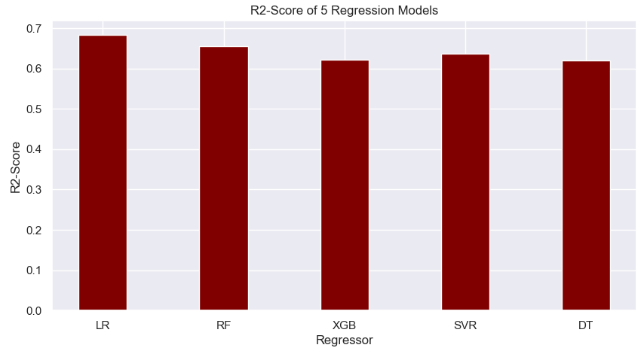
- Comparison of R2-score for 5 regression models
import numpy as np
import matplotlib.pyplot as plt


# creating the dataset
data = {'LR':0.684, 'RF':0.656, 'XGB':0.621,
        'SVR':0.637,'DT':0.620}
courses = list(data.keys())
values = list(data.values())

fig = plt.figure(figsize = (10, 5))

# creating the bar plot
plt.bar(courses, values, color ='maroon',
        width = 0.4)

plt.xlabel("Regressor")
plt.ylabel("R2-Score")
plt.title("R2-Score of 5 Regression Models")
plt.show()
Project 2: Tuned RF Regression of Prices
- Preparing the input data for Random Forest (RF) regression of AMS house prices in 2021
import numpy as np # linear algebra
import pandas as pd # data processing, CSV file I/O (e.g. pd.read_csv)
import warnings
warnings.filterwarnings('ignore')
import matplotlib.pyplot as plt
import seaborn as sns
from sklearn.model_selection import cross_val_score
from sklearn.metrics import mean_squared_error
df = pd.read_csv('HousingPrices-Amsterdam-August-2021.csv')
df = df.dropna(axis = 0, inplace = False)
q1 = df.describe()['Price']['25%']
q3 = df.describe()['Price']['75%']
iqr = q3 - q1
max_price = q3 + 1.5 * iqr
outliers = df[df['Price'] >= max_price]
outliers_count = outliers['Price'].count()
df_count = df['Price'].count()
print('Percentage removed: ' + str(round(outliers_count/df_count * 100, 2)) + '%')
Percentage removed: 7.72%
df= df[df['Price'] <= max_price]
df['Zip No'] = df['Zip'].apply(lambda x:x.split()[0])
df['Letters'] = df['Zip'].apply(lambda x:x.split()[-1])
def word_separator(string):
    list = string.split()
    word = []
    number = []
    for element in list:
        if element.isalpha() == True:
            word.append(element)
        else:
            break
    word = ' '.join(word)
    return word
df['Street'] = df['Address'].apply(lambda x:word_separator(x))
numerical = ['Price', 'Area', 'Room', 'Lon', 'Lat']
categorical = ['Address', 'Zip No', 'Letters', 'Street']
- Applying Label Encoding to categorical data and dropping unused columns
from sklearn.preprocessing import LabelEncoder
for c in categorical:
    lbl = LabelEncoder()
    lbl.fit(list(df[c].values))
    df[c] = lbl.transform(list(df[c].values))

df.drop(['Zip', 'Unnamed: 0', 'Address'], axis =1, inplace = True)
- Train/test data splitting and scaling
from sklearn.model_selection import train_test_split
X = df.drop('Price', axis =1)
y = df['Price']
X_train, X_test, y_train, y_test = train_test_split(X,y, test_size = 0.2)
from sklearn.preprocessing import StandardScaler
scaler = StandardScaler()
X_train = scaler.fit_transform(X_train)
X_test = scaler.transform(X_test)
- Applying RandomizedSearchCV to RandomForestRegressor
from sklearn.model_selection import RandomizedSearchCV, GridSearchCV

random_grid = {'bootstrap': [True, False],
 'max_depth': [10, 20, 30, 40, 50, 60, 70, 80, 90, 100, None],
 'max_features': ['auto', 'sqrt'],
 'min_samples_leaf': [1, 2, 4],
 'min_samples_split': [2, 5, 10],
 'n_estimators': [200, 400, 600, 800, 1000, 1200, 1400, 1600, 1800, 2000]}

random_cv = RandomizedSearchCV(estimator = random_forest, param_distributions = random_grid, n_iter = 100, cv = 10, verbose = 2, n_jobs = -1)
random_cv.fit(X_train, y_train)
Fitting 10 folds for each of 100 candidates, totalling 1000 fits

  RandomizedSearchCV
estimator: RandomForestRegressor

 RandomForestRegressor
- Getting the best hyperparameters
random_cv.best_params_

{'n_estimators': 1600,
 'min_samples_split': 2,
 'min_samples_leaf': 1,
 'max_features': 'sqrt',
 'max_depth': 70,
 'bootstrap': False}
- Training the tuned RF model
tuned_random_forest = RandomForestRegressor(n_estimators = 1600, max_depth = 70, min_samples_leaf = 1, min_samples_split = 2)
random_forest.fit(X_train, y_train)
predictions = random_forest.predict(X_test)
cv = cross_val_score(tuned_random_forest, X_train, y_train, cv=20, scoring = 'neg_mean_squared_error')
print("The Random Forest Regressor with tuned parameters has a RMSE of: " + str(abs(cv.mean())**0.5))
The Random Forest Regressor with tuned parameters has a RMSE of: 92683.47375648536

# Calculate testing scores
from sklearn.metrics import mean_absolute_error, r2_score
test_mae = mean_absolute_error(y_test, predictions)
test_mse = mean_squared_error(y_test, predictions)
test_rmse = mean_squared_error(y_test, predictions, squared=False)
test_r2 = r2_score(y_test, predictions)
print(test_mae)
60217.95247058822
print(test_mse)
7459469611.399326
print(test_rmse)
86368.22107349048
print(test_r2)
0.8544722257795427
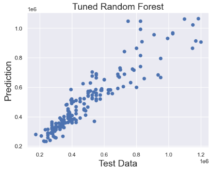
- Plotting test data vs tuned RF predictions
plt.scatter(y_test,predictions)
plt.title('Tuned Random Forest',fontsize=18)
plt.xlabel('Test Data',fontsize=18)
plt.ylabel('Prediction',fontsize=18)
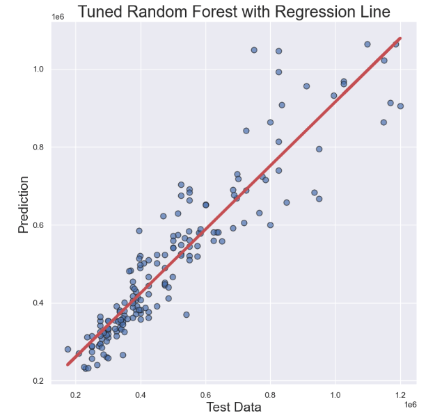
- Finally, let’s make the scatter X-plot, and add the regression line:
# Generate data
x = y_test
y = predictions

# Initialize layout
fig, ax = plt.subplots(figsize = (9, 9))

# Add scatterplot
ax.scatter(x, y, s=60, alpha=0.7, edgecolors="k")

# Fit linear regression via least squares with numpy.polyfit
# It returns an slope (b) and intercept (a)
# deg=1 means linear fit (i.e. polynomial of degree 1)
b, a = np.polyfit(x, y, deg=1)

# Create sequence
xseq = x

# Plot regression line
ax.plot(xseq, a + b * xseq, color="r", lw=4);
plt.xlabel('Test Data',fontsize=18)
plt.ylabel('Prediction',fontsize=18)
plt.title('Tuned Random Forest with Regression Line',fontsize=22)
Conclusions
- As data scientists, we have the power to revolutionize the REIT by developing models that can accurately analyze the real estate market trends while predicting house prices.
- In this study, we have chosen Amsterdam (AMS) as the key place to focus on, and we are estimating the current market value of REIT in a number of different neighborhoods.
- Project 1 reports on the comprehensive Exploratory Data Analysis (EDA) of the summary information and metrics for listings as well as ML regression of review scores in AMS.
- Project 2 utilizes various features to predict housing prices in and around AMS using the Kaggle dataset.
- Through descriptive statistics, we gain insight into the central tendencies and distributions of our data, while correlation analysis helps us to understand the relationships between different variables.
- Our ML approach encompasses regression, model tuning and NLP algorithms deployed to facilitate investments, enhance property management, and improve customer experience in AMS real estate & REIT.
- Trained with historical data, our ML systems can recognize patterns and relationships among multiple variables to predict how such parameters will affect the price-to-rent ratio, property sale price, and review scores of tenants bringing transparency to the rental market.
- This case study has confirmed the great business value of data science applications in real estate that can help companies get real-time information on customer needs and interests, property valuation, and local market insights.
- We have shown that real estate investors can get some excellent benefits of data science such as optimized profits vs risks, improved competitive advantage, automated operations, and increased employee efficiency.
Explore More
- About MLOps
- US Real Estate – Harnessing the Power of AI
- WA House Price Prediction: EDA-ML-HPO
- Real Estate Supervised ML/AI Linear Regression Revisited – USA House Price Prediction
- Supervised Machine Learning Use Case: Prediction of House Prices
References
- Airbnb: The Amsterdam story with interactive maps
- Amsterdam Inside Airbnb EDA
- Amsterdam House Price Prediction
- Amsterdam House Prices
- Amsterdam house price prediction
- Machine Learning and Real State: Predicting Rental Prices in Amsterdam
- Going Dutch: How I Used Data Science and Machine Learning to Find an Apartment in Amsterdam — Part I
Embed Socials
Infographics
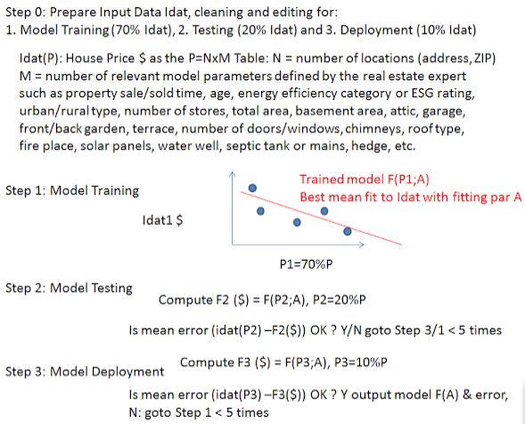
- Real estate ML regression algorithm explained.
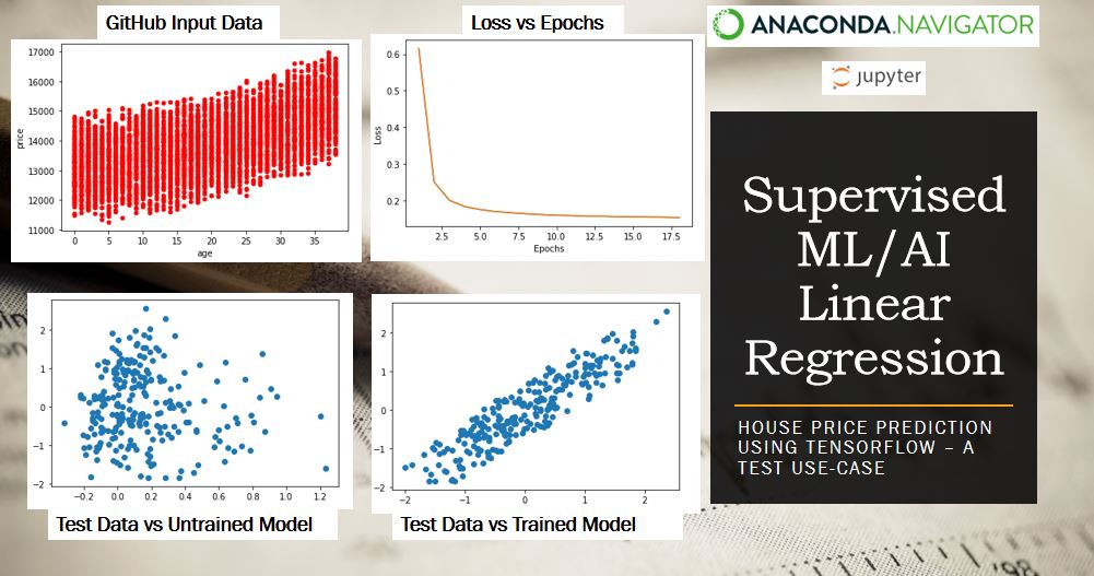
- Supervised ML/AI linear regression of house prices: TensorFlow demo.
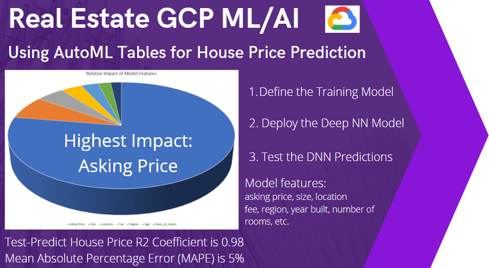
- Real estate GCP ML/AI workflow deployed.
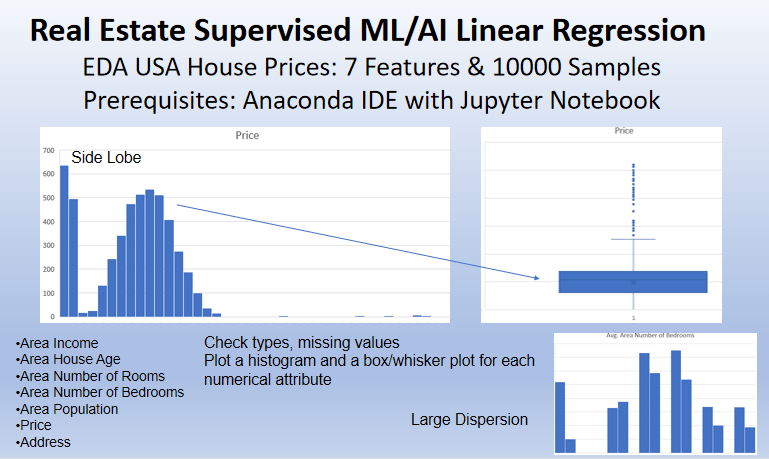
- Real estate supervised ML/AI linear regression: USA house prices demo example
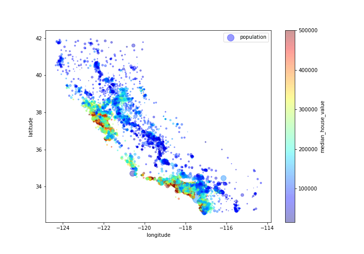
- CA median house value, population and geospatial map


Make a one-time donation
Make a monthly donation
Make a yearly donation
Choose an amount
Or enter a custom amount
Your contribution is appreciated.
Your contribution is appreciated.
Your contribution is appreciated.

Leave a comment