
- The objective of this study is to evaluate sales and demand forecasting methods to help retail businesses make sense of market trends and provide the best possible offering to their customers. In fact, for sales forecasting is a large part of supply chain planning, as the chains only provide what retailers think the customers will want.
- Time-series analysis (TSA) is an effective statistical approach for predicting sales based on historical data, allowing retailers to make data-driven decisions and enhance operational efficiency.
- Referring to the multiple TSA case study and the corresponding algorithm, we train and evaluate the FB Prophet models with cross-validation and hyper-parameter optimization (Part 1). We will examine the impact of adding change points, seasonality, and events to these TSA models.
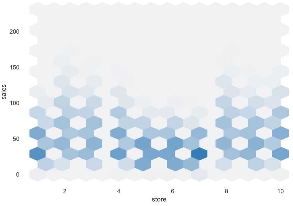
- We download the first input Kaggle dataset that has 10 different stores and each store has 50 items, i.e. total of 500 daily level time series data for 5 years. We analyze and investigate this dataset using the Pandas Profiling and SWEETVIZ AutoEDA HTML reports.
- In the second part of the post, the focus is on ARIMA models and their variants SARIMA and SARIMAX. These are widely recognized and extensively utilized TSA models.
- The aim is to unlock the power of the SARIMAX TSA in comparison with the FB Prophet, ARIMA and SARIMA predictions. In this example, we use a part of the input data that can be found here.
- To help us understand the accuracy of TSA, we compare predicted sales to real sales of the time series.
- FB Prophet X-validation plots consist of the trend, seasonal components, MAE and MAPE between expected and predicted values.
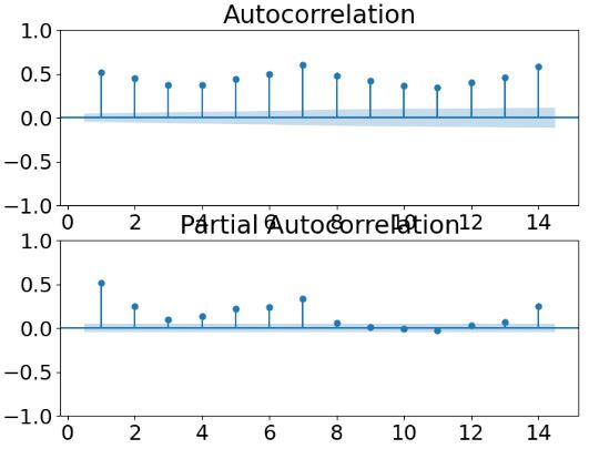
- The autocorrelation analysis (ACF and PACF) helps detect patterns and check for randomness.
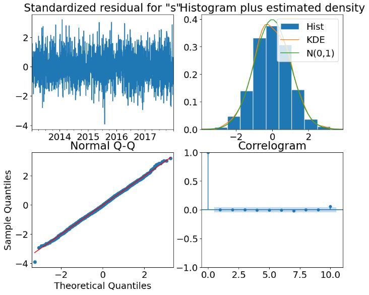
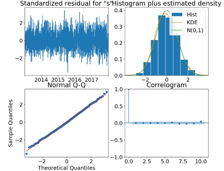
- In addition to correlograms, ARIMA diagnostics plots contain standardized residuals, normal Q-Q, and histogram + estimated density.
- Points on the Normal Q-Q plot provide an indication of univariate normality of the dataset. Read more here.
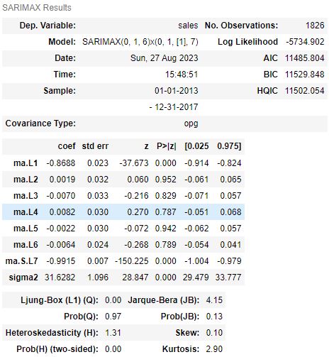
- The Statsmodels’ SARIMAX QC tables can help you determine whether our SARIMAX model can actually yield meaningful information. These tables contain the following statistical metrics: Log Likelihood, AIC, BIC, HQIC, Ljung-Box, JB, H, Prob, Skew, and Kurtosis.
Table of Contents
AutoEDA
- Let’s set the working directory ARL and import the basic libraries
import os
os.chdir('ARL')    # Set working directory
os. getcwd()
%matplotlib inline

import pandas as pd
import numpy as np
import matplotlib.pyplot as plt
- Reading the input data
data = pd.read_csv("trainretail.csv", index_col=0)
data = data.reset_index()
data.head()
date	store	item	sales
0	2013-01-01	1	1	13
1	2013-01-02	1	1	11
2	2013-01-03	1	1	14
3	2013-01-04	1	1	13
4	2013-01-05	1	1	10

print(f"The dataset has {data.shape[0]} rows and {data.shape[1]} columns")
The dataset has 913000 rows and 4 columns
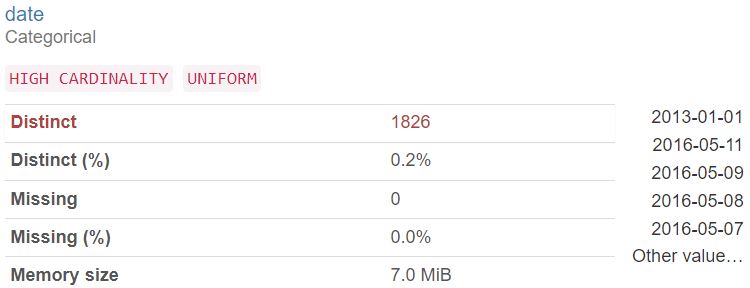
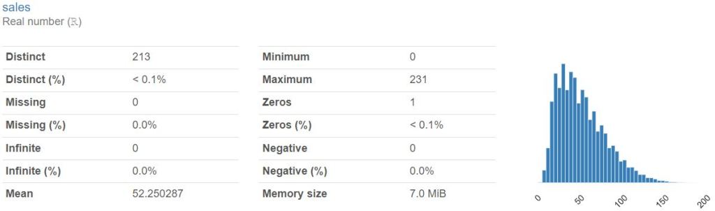
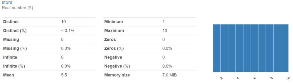
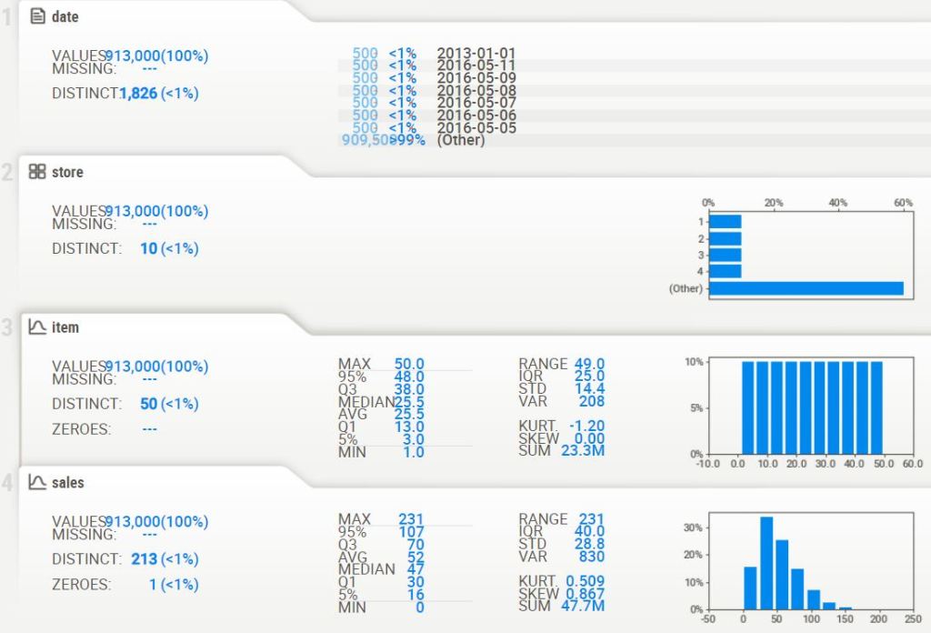
- Generating the Pandas Profiling Report
import pandas as pd
from pandas_profiling import ProfileReport

profile = ProfileReport(data, title="Pandas Profiling Report")
profile.to_file("reportretail.html")
Variables:

Interactions:
Correlations: store item sales
| store | 1.000 | 0.000 | -0.007 |
|---|---|---|---|
| item | 0.000 | 1.000 | -0.054 |
| sales | -0.007 | -0.054 | 1.000 |
Alerts:
date has a high cardinality: 1826 distinct values | High cardinality |
date is uniformly distributed |
- Generating the sweetviz report
import sweetviz as sv
import pandas as pd

# Create an analysis report for your data
report = sv.analyze(data)

# Display the report
report.show_html()

Variables
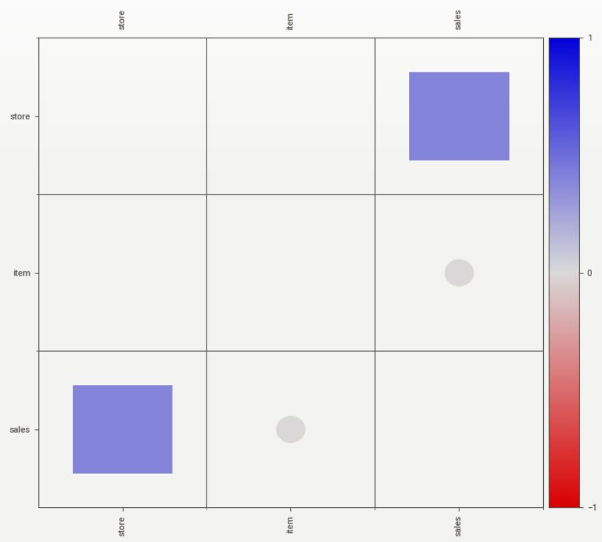
Associations
[Only including dataset “DataFrame”]
■ Squares are categorical associations (uncertainty coefficient & correlation ratio) from 0 to 1. The uncertainty coefficient is assymmetrical, (i.e. ROW LABEL values indicate how much they PROVIDE INFORMATION to each LABEL at the TOP).
• Circles are the symmetrical numerical correlations (Pearson’s) from -1 to 1. The trivial diagonal is intentionally left blank for clarity.
FB Prophet
- Preparing the input data for TSA
import itertools

multiindex = list(zip(item_sales_per_date["date"], item_sales_per_date["store_item"]))
multiindex = pd.MultiIndex.from_tuples(multiindex, names=('index_1', 'index_2'))

dataset = item_sales_per_date.copy()
dataset.index = multiindex


idx_dates = list(pd.date_range(min(item_sales_per_date["date"]), max(item_sales_per_date["date"])))
idx_ids = list(dataset["store_item"].unique())
idx = list(itertools.product(idx_dates, idx_ids))
dataset = dataset.reindex(idx)
dataset = dataset.reset_index()
dataset.head()
index_1	index_2	date	store_item	sales
0	2013-01-01	1_1	2013-01-01	1_1	13
1	2013-01-01	2_3	2013-01-01	2_3	19
2	2013-01-01	2_29	2013-01-01	2_29	50
3	2013-01-01	2_28	2013-01-01	2_28	45
4	2013-01-01	2_27	2013-01-01	2_27	17

dataset["date"] = dataset["date"].fillna(dataset["index_1"])
dataset["store_item"] = dataset["store_item"].fillna(dataset["index_2"])
dataset["sales"] = dataset["sales"].fillna(0)
dataset = dataset.drop(columns=["index_1", "index_2"])
dataset = dataset.set_index("date")
dataset.index.name = "date"
dataset.head()
store_item	sales
date
2013-01-01	1_1	13
2013-01-01	2_3	19
2013-01-01	2_29	50
2013-01-01	2_28	45
2013-01-01	2_27	17
- Renaming the columns as follows
# The 'store_item' becomes 'unique_id' representing the unique identifier of the time series
# The 'date' becomes 'ds' representing the time stamp of the data points
# The 'sales' becomes 'y' representing the target variable we want to forecast
# Y_df = dataset.query('unique_id.str.startswith("6_46")').copy()
Y_df = dataset.copy()
Y_df = Y_df.reset_index()
Y_df = Y_df.rename(columns={
    'store_item': 'unique_id',
    'date': 'ds',
    'sales': 'y'
})
Y_df['y'] = Y_df['y'].astype(int)
# Convert the 'ds' column to datetime format to ensure proper handling of date-related operations in subsequent steps
Y_df['ds'] = pd.to_datetime(Y_df['ds'])


Y_df['unique_id'] = Y_df['unique_id'].astype(str)

Y_df.tail()
ds	unique_id	y
182595	2017-12-31	1_36	71
182596	2017-12-31	1_35	55
182597	2017-12-31	1_34	32
182598	2017-12-31	1_33	61
182599	2017-12-31	1_42	27
- Running the FB Prophet TSA with 95% confidence
# Import Prophet
from prophet import Prophet
## Creating model parameters
model_param ={
    "daily_seasonality": False,
    "weekly_seasonality":False,
    "yearly_seasonality":True,
    "seasonality_mode": "multiplicative",
    "growth": "logistic"
}
Y_df['cap']= Y_df["y"].max() + Y_df["y"].std() * 0.05
# Setting a cap or upper limit for the forecast as we are using logistics growth
# The cap will be maximum value of target variable plus 5% of std.
model = Prophet(**model_param)
model.fit(Y_df)

# Create future dataframe
future= model.make_future_dataframe(periods=365)
future['cap'] = Y_df['cap'].max()

forecast= model.predict(future)
- Plotting the FB Prophet components and the forecast output
model.plot_components(forecast);
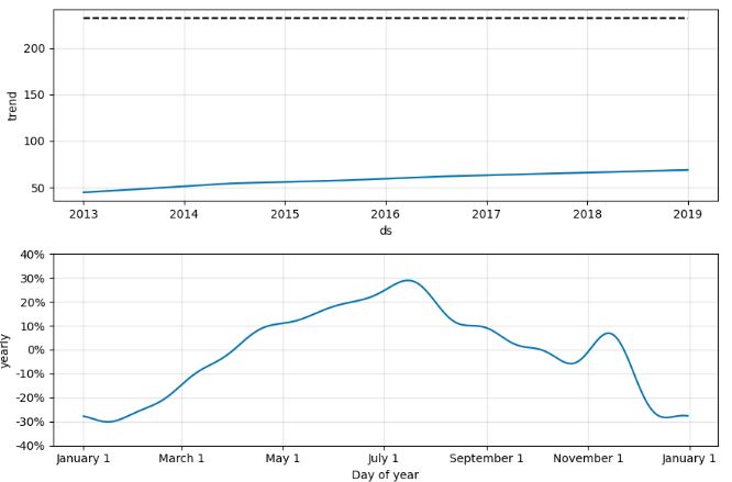
model.plot(forecast);# black dots are actual values and blue dots are forecast

- Adding extra parameters related to seasonality and events
## Adding parameters and seasonality and events
model = Prophet(**model_param)

model= model.add_seasonality(name="monthly", period=30, fourier_order=10)
model= model.add_seasonality(name="quarterly", period=92.25, fourier_order=10)

model.add_country_holidays("US")

model.fit(Y_df)

# Create future dataframe
future= model.make_future_dataframe(periods=365)
future['cap'] = Y_df['cap'].max()

forecast= model.predict(future)


- Selecting store 2 and item 28 subset of the input data
import pandas as pd
import numpy as np
import matplotlib.pyplot as plt

import statsmodels.api as sm
from sklearn.metrics import mean_absolute_error, mean_absolute_percentage_error
from prophet import Prophet

import warnings
warnings.filterwarnings('ignore')
pd.set_option('display.width', None)
pd.set_option('display.max_rows', None)
df_store_2_item_28 = pd.read_csv("sales_store_2_item_28.csv")
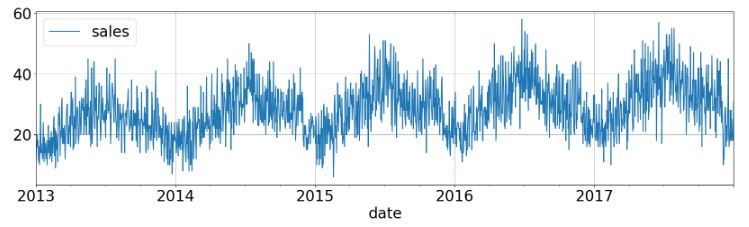
- Plotting the time-series data
import matplotlib
plt.figure(figsize=(15, 6))
matplotlib.rcParams.update({'font.size': 24})
df_store_2_item_28['date']=pd.to_datetime(df_store_2_item_28['date'])
df_store_2_item_28_time = df_store_2_item_28.set_index('date')
# Plot the entire time series data
df_store_2_item_28_time.plot(grid=True,figsize=(20,5))
plt.show()
- Plotting the monthly resampled data
df_store_2_item_28_time.resample('M').sum().plot(grid=True,figsize=(20,5))
plt.show()

- Plotting the yearly resampled data
df_store_2_item_28_time.resample('A').sum().plot(grid=True,figsize=(20,5))
plt.show()

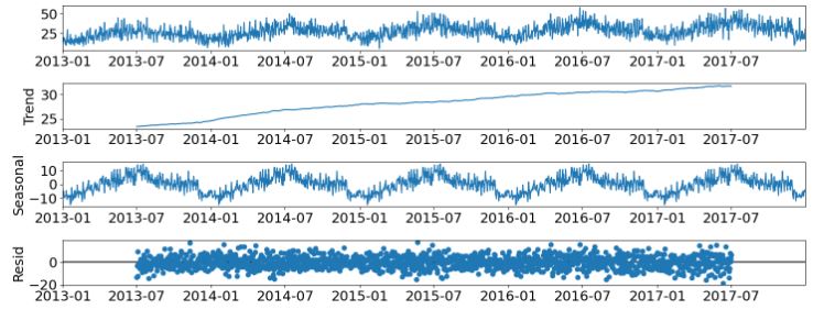
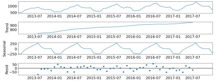
- Performing the statsmodels seasonal additive decomposition of original and resampled data
from pylab import rcParams
matplotlib.rcParams.update({'font.size': 18})
rcParams['figure.figsize'] = 15, 6
decomposition = sm.tsa.seasonal_decompose(df_store_2_item_28_time,
                                         model = 'additive',
                                         period=365)
fig = decomposition.plot()
plt.show()
decomposition = sm.tsa.seasonal_decompose(df_store_2_item_28_time.resample('M').sum(),
                                          model = 'additive',
                                         period=12)
fig = decomposition.plot()
plt.show()
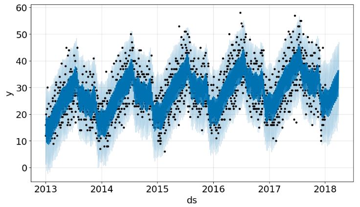
- Forecasting with FB Prophet (periods=90 and interval_width=0.95)
# rename date and sales, respectively ds and y
df_store_2_item_28.columns = ['ds','y']
m = Prophet(interval_width=0.95) #by default is 80%
model = m.fit(df_store_2_item_28)
future = m.make_future_dataframe(periods=90)
forecast = m.predict(future)
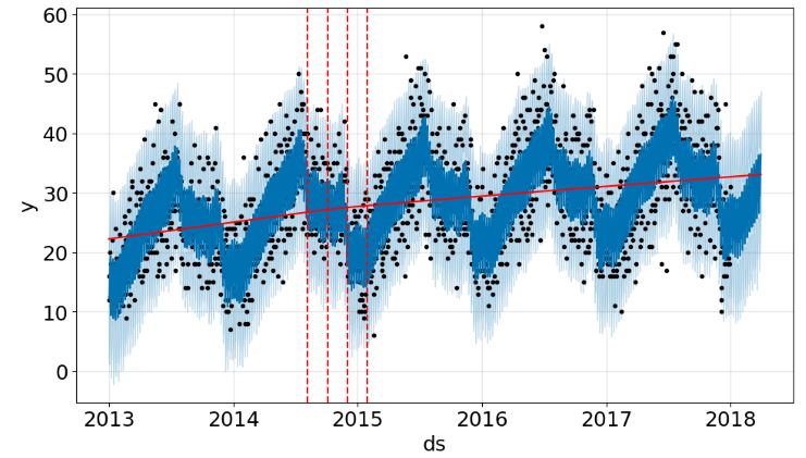
plot1 = m.plot(forecast)
- Adding change points to the above plot
from prophet.plot import add_changepoints_to_plot

plot1 = m.plot(forecast)
a = add_changepoints_to_plot(plot1.gca(),m,forecast)
- Plotting the subset components
plot2 = m.plot_components(forecast)

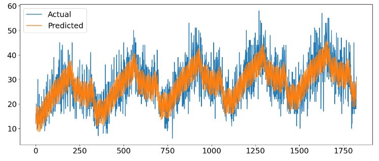
- Plotting the key FB Prophet (model 1) X-validation diagnostics – yhat, MAE, and MAPE
df_merge = pd.merge(df_store_2_item_28, forecast[['ds','yhat_lower','yhat_upper','yhat']],on='ds')
df_merge = df_merge[['ds','yhat_lower','yhat_upper','yhat','y']]
# calculate MAE between observed and predicted values
y_true = df_merge['y'].values
y_pred = df_merge['yhat'].values
mae_01 = mean_absolute_error(y_true, y_pred)
print('MAE: %.3f' % mae_01)
MAE: 4.275
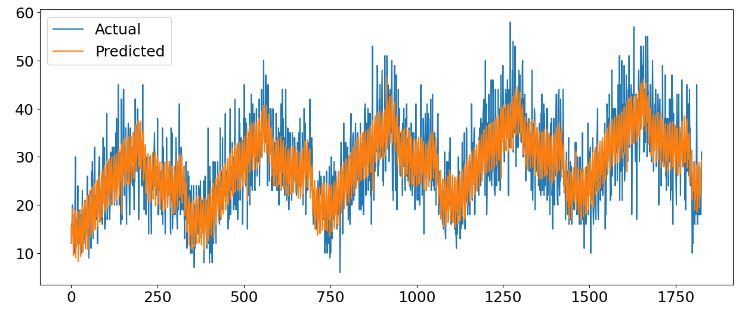
# plot expected vs actual
plt.plot(y_true, label='Actual')
plt.plot(y_pred, label='Predicted')
plt.legend()
plt.show()
- FB Prophet X-validation
from prophet.diagnostics import cross_validation
df_cv = cross_validation(m, horizon='90 days')
INFO:prophet:Making 31 forecasts with cutoffs between 2014-01-21 00:00:00 and 2017-10-02 00:00:00
- Calculating the key performance metrics
from prophet.diagnostics import performance_metrics
df_p = performance_metrics(df_cv)
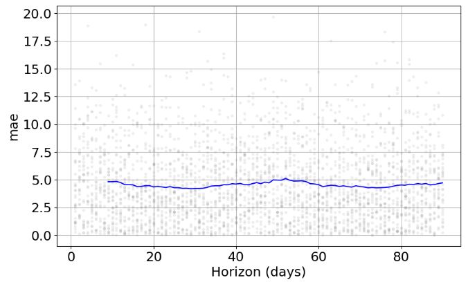
- Plotting MAE
from prophet.plot import plot_cross_validation_metric

plot3 = plot_cross_validation_metric(df_cv, metric='mae')
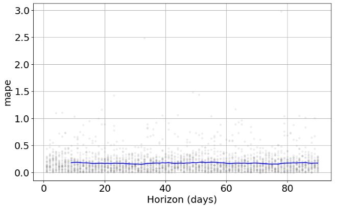
- Plotting MAPE
plot4 = plot_cross_validation_metric(df_cv, metric='mape')
- Storing the calculated metrics (model 1) in metrics_prophet_01
y_true = df_merge['y'].values
y_pred = df_merge['yhat'].values
mae_01 = mean_absolute_error(y_true, y_pred)
print('MAE: %.3f' % mae_01)
MAE: 4.252
mape_01 = mean_absolute_percentage_error(y_true, y_pred)
print('MAPE: %.3f' % mape_01)
MAPE: 0.168
metrics_prophet_01 = [round(mae_01,3),
                 round(mape_01,3)]
- Fine tuning hyperparameters by generating all combinations of parameters while minimizing MAE and MAPE
import itertools

param_grid = {
    'changepoint_prior_scale': [0.001, 0.01, 0.1, 0.5],
    'seasonality_prior_scale': [0.01, 0.1, 1.0, 10.0],
}

# Generate all combinations of parameters
all_params = [dict(zip(param_grid.keys(), v)) for v in itertools.product(*param_grid.values())]
maes = []  # Store the MAE for each params here
mapes = [] # Store the MAPE for each params here

# Use cross validation to evaluate all parameters
for params in all_params:
    m = Prophet(**params).fit(df_store_2_item_28)  # Fit model with given params
    df_cv = cross_validation(m, horizon='90 days', parallel="processes")
    df_p = performance_metrics(df_cv, rolling_window=1)
    maes.append(df_p['mae'].values[0])
    mapes.append(df_p['mape'].values[0])

# Find the best parameters
tuning_results = pd.DataFrame(all_params)
tuning_results['mae'] = maes
tuning_results['mape'] = mapes
tuning_results_df = pd.DataFrame(tuning_results)
tuning_results_df.sort_values(['mae','mape'])
- Finding the best parameters and generating TSA model 2
best_params = all_params[np.argmin(mapes)]
print(best_params)
{'changepoint_prior_scale': 0.1, 'seasonality_prior_scale': 10.0}
m = Prophet(interval_width=0.95, weekly_seasonality=True,
            changepoint_prior_scale=best_params['changepoint_prior_scale'],
            seasonality_prior_scale=best_params['seasonality_prior_scale'])
model = m.fit(df_store_2_item_28)
future = m.make_future_dataframe(periods=90) #to predict 90 days in the future
forecast = m.predict(future)
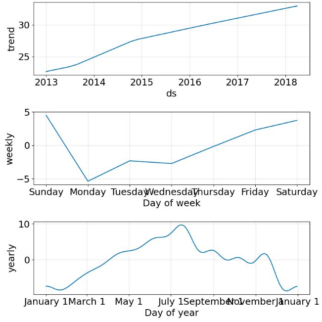
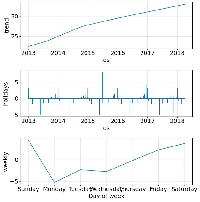
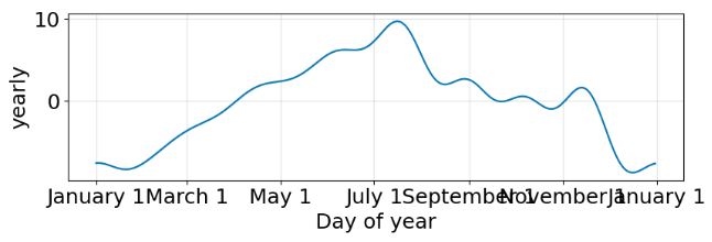
- Plotting the TSA forecast and key components of model 2
plot5 = m.plot(forecast)
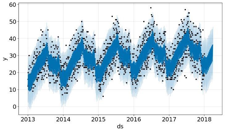
plot6 = m.plot_components(forecast)
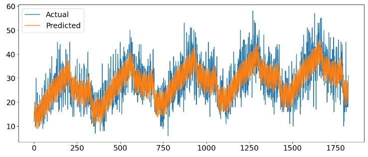
- Calculating the key performance metrics and storing them in metrics_prophet_02, running X-validation and plotting time-series comparisons (model 2)
df_merge = pd.merge(df_store_2_item_28, forecast[['ds','yhat_lower','yhat_upper','yhat']],on='ds')
df_merge = df_merge[['ds','yhat_lower','yhat_upper','yhat','y']]
y_true = df_merge['y'].values
y_pred = df_merge['yhat'].values
mae_02 = mean_absolute_error(y_true, y_pred)
print('MAE: %.3f' % mae_02)
MAE: 4.269
mape_02 = mean_absolute_percentage_error(y_true, y_pred)
print('MAPE: %.3f' % mape_02)
MAPE: 0.168
# plot expected vs actual
plt.plot(y_true, label='Actual')
plt.plot(y_pred, label='Predicted')
plt.legend()
plt.show()
df_cv = cross_validation(m, horizon='90 days')
df_p = performance_metrics(df_cv)
plot7 = plot_cross_validation_metric(df_cv, metric='mape')

- Adding the US holidays as events to the tuned model (model 3)
m = Prophet(interval_width=0.95, weekly_seasonality=True,
            changepoint_prior_scale=best_params['changepoint_prior_scale'],
            seasonality_prior_scale=best_params['seasonality_prior_scale'])
m.add_country_holidays(country_name='US')
model = m.fit(df_store_2_item_28)
# holidays included
m.train_holiday_names
0                  New Year's Day
1      Martin Luther King Jr. Day
2           Washington's Birthday
3                    Memorial Day
4                Independence Day
5                       Labor Day
6                    Columbus Day
7                    Veterans Day
8                    Thanksgiving
9                   Christmas Day
10       Christmas Day (Observed)
11      New Year's Day (Observed)
12        Veterans Day (Observed)
13    Independence Day (Observed)
dtype: object
future = m.make_future_dataframe(periods=90)
forecast = m.predict(future)
- Plotting the TSA forecast and key components of model 3
plot5 = m.plot(forecast)
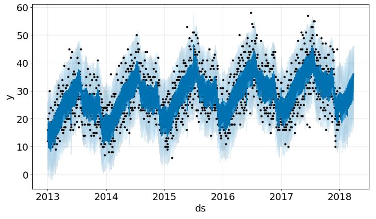
plot6 = m.plot_components(forecast)
- Calculating the key performance metrics and storing them in metrics_prophet_03, running X-validation and plotting time-series comparisons (model 3)
df_merge = pd.merge(df_store_2_item_28, forecast[['ds','yhat_lower','yhat_upper','yhat']],on='ds')
df_merge = df_merge[['ds','yhat_lower','yhat_upper','yhat','y']]
# calculate MAE between expected and predicted values
y_true = df_merge['y'].values
y_pred = df_merge['yhat'].values
mae_03 = mean_absolute_error(y_true, y_pred)
print('MAE: %.3f' % mae_03)
MAE: 4.252
mape_03 = mean_absolute_percentage_error(y_true, y_pred)
print('MAPE: %.3f' % mape_03)
MAPE: 0.168
# plot expected vs actual
plt.plot(y_true, label='Actual')
plt.plot(y_pred, label='Predicted')
plt.legend()
plt.show()
df_cv = cross_validation(m, horizon='90 days')
metrics_prophet_03 = [round(mae_03,3),
                 round(mape_03,3)]
- Printing the final FB Prophet TSA summary for models 1-3
pd.DataFrame({'metrics':['MAE','MAPE'],
              'Prophet_01':metrics_prophet_01,
              'Prophet_02':metrics_prophet_02,
              'Prophet_03':metrics_prophet_03,
             })
metrics	Prophet_01	Prophet_02	Prophet_03
0	MAE	    4.252	4.269	4.252
1	MAPE	0.168	0.168	0.168
- It is clear that neither model tuning nor adding extra events provides significantly better prediction accuracy. Which approach should we follow to minimize MAE and MAPE?
SARIMAX
- Defining the input dataset and searching for optimal SARIMAX order parameters p and q using AIC and BIC
df_store_2_item_28 = pd.read_csv("sales_store_2_item_28.csv")
# set date as index
df_store_2_item_28_time = df_store_2_item_28.set_index('date')
df_store_2_item_28_time.index = pd.DatetimeIndex(df_store_2_item_28_time.index.values)
# Create empty list to store search results
order_aic_bic=[]

# Loop over p values from 0-6
for p in range(7):
  # Loop over q values from 0-6
    for q in range(7):
      	# create and fit ARMA(p,q) model
        model = SARIMAX(df_store_2_item_28_time, order=(p,1,q), freq="D") #because adf test showed that d=1
        results = model.fit()

        # Append order and results tuple
        order_aic_bic.append((p,q,results.aic, results.bic))

# Construct DataFrame from order_aic_bic
order_df = pd.DataFrame(order_aic_bic,
                        columns=['p','q','AIC','BIC'])

# Print order_df in order of increasing AIC
order_df.sort_values('AIC')

p	q	AIC	BIC
33	4	5	11671.554531	11726.647884
40	5	5	11672.383126	11732.985814
34	4	6	11683.272060	11743.874748
48	6	6	11708.930745	11780.552103
41	5	6	11719.959572	11786.071595
26	3	5	11723.712296	11773.296313
32	4	4	11725.330619	11774.914637
47	6	5	11726.087503	11792.199526
27	3	6	11729.544932	11784.638285

# Print order_df in order of increasing BIC
order_df.sort_values('BIC')
	p	q	AIC	BIC
33	4	5	11671.554531	11726.647884
40	5	5	11672.383126	11732.985814
34	4	6	11683.272060	11743.874748
18	2	4	11729.819753	11768.385100
24	3	3	11731.213716	11769.779063
26	3	5	11723.712296	11773.296313
32	4	4	11725.330619	11774.914637
25	3	4	11730.958579	11775.033261
48	6	6	11708.930745	11780.552103
20	2	6	11733.878491	11783.462508
19	2	5	11739.689796	11783.764478
27	3	6	11729.544932	11784.638285
41	5	6	11719.959572	11786.071595
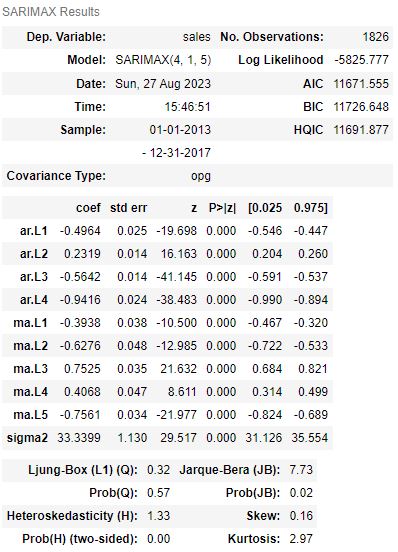
- Fitting the optimized model, calculating MAE and printing the summary diagnostics
arima_model = SARIMAX(df_store_2_item_28_time, order=(4,1,5))
# fit model
arima_results = arima_model.fit()

# Calculate the mean absolute error from residuals
mae = np.mean(np.abs(arima_results.resid))

# Print mean absolute error
print('MAE: %.3f' % mae)
MAE: 4.737
arima_results.summary()
- Creating the 4 diagnostics plots using plot_diagnostics for the above model
- Computing ACF and PACF for the SARIMAX(4,1,5) model
# Create the figure
fig, (ax1, ax2) = plt.subplots(2,1,figsize=(8,6))

# Plot the ACF on ax1
plot_acf(df_store_2_item_28_time, lags=14, zero=False, ax=ax1)

# Plot the PACF on ax2
plot_pacf(df_store_2_item_28_time, lags=14, zero=False, ax=ax2)

plt.show()
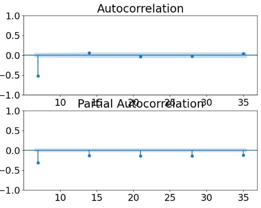
- Transformation to stationary data by taking the first and seasonal differences (S=7) and dropping Nan’s
df_store_2_item_28_time_diff = df_store_2_item_28_time.diff().diff(7).dropna()
# Make list of lags
lags = [7, 14, 21, 28, 35]

# Create the figure
fig, (ax1, ax2) = plt.subplots(2,1,figsize=(8,6))

# Plot the ACF on ax1
plot_acf(df_store_2_item_28_time_diff, lags=lags, zero=False, ax=ax1)

# Plot the PACF on ax2
plot_pacf(df_store_2_item_28_time_diff, lags=lags, zero=False, ax=ax2)

plt.show()
- Creating the 2nd SARIMAX model with order=(0,1,6), seasonal_order=(0,1,1,7)
sarima_01_model = SARIMAX(df_store_2_item_28_time, order=(0,1,6), seasonal_order=(0,1,1,7))
sarima_01_results = sarima_01_model.fit()

# Calculate the mean absolute error from residuals
mae = np.mean(np.abs(sarima_01_results.resid))

# Print mean absolute error
print('MAE: %.3f' % mae)
MAE: 4.555
- Printing the SARIMAX summary for the above model
sarima_01_results.summary()
- Creating the 4 diagnostics plots using plot_diagnostics for the 2nd SARIMAX model
- Creating the Auto ARIMA model by performing stepwise search to minimize AIC
import pmdarima as pm

# Create auto_arima model
model1 = pm.auto_arima(df_store_2_item_28_time, #time series
                      seasonal=True, # is the time series seasonal
                      m=7, # the seasonal period - one week?
                      d=1, # non-seasonal difference order
                      D=1, # seasonal difference order
                 	  max_p=6, # max value of p to test
                      max_q=6, # max value of p to test
                      max_P=6, # max value of P to test
                      max_Q=6, # max value of Q to test
                      information_criterion='aic', # used to select best mode
                      trace=True, # prints the information_criterion for each model it fits
                      error_action='ignore', # ignore orders that don't work
                      stepwise=True, # apply an intelligent order search
                      suppress_warnings=True)

# Print model summary
print(model1.summary())

Performing stepwise search to minimize aic
 ARIMA(2,1,2)(1,1,1)[7]             : AIC=inf, Time=3.88 sec
 ARIMA(0,1,0)(0,1,0)[7]             : AIC=13739.527, Time=0.03 sec
 ARIMA(1,1,0)(1,1,0)[7]             : AIC=12650.572, Time=0.17 sec
 ARIMA(0,1,1)(0,1,1)[7]             : AIC=inf, Time=0.64 sec
 ARIMA(1,1,0)(0,1,0)[7]             : AIC=13229.902, Time=0.06 sec
 ARIMA(1,1,0)(2,1,0)[7]             : AIC=12480.179, Time=0.31 sec
 ARIMA(1,1,0)(3,1,0)[7]             : AIC=12344.238, Time=0.71 sec
 ARIMA(1,1,0)(4,1,0)[7]             : AIC=12270.400, Time=1.12 sec
 ARIMA(1,1,0)(5,1,0)[7]             : AIC=12224.430, Time=1.57 sec
 ARIMA(1,1,0)(6,1,0)[7]             : AIC=12196.670, Time=2.79 sec
 ARIMA(1,1,0)(6,1,1)[7]             : AIC=inf, Time=22.80 sec
 ARIMA(1,1,0)(5,1,1)[7]             : AIC=inf, Time=16.60 sec
 ARIMA(0,1,0)(6,1,0)[7]             : AIC=12702.277, Time=2.00 sec
 ARIMA(2,1,0)(6,1,0)[7]             : AIC=11998.566, Time=2.86 sec
 ARIMA(2,1,0)(5,1,0)[7]             : AIC=12027.447, Time=2.37 sec
 ARIMA(2,1,0)(6,1,1)[7]             : AIC=inf, Time=24.39 sec
 ARIMA(2,1,0)(5,1,1)[7]             : AIC=inf, Time=18.97 sec
 ARIMA(3,1,0)(6,1,0)[7]             : AIC=11888.959, Time=4.14 sec
 ARIMA(3,1,0)(5,1,0)[7]             : AIC=11915.280, Time=2.62 sec
 ARIMA(3,1,0)(6,1,1)[7]             : AIC=inf, Time=32.36 sec
 ARIMA(3,1,0)(5,1,1)[7]             : AIC=inf, Time=21.27 sec
 ARIMA(4,1,0)(6,1,0)[7]             : AIC=11829.853, Time=3.99 sec
 ARIMA(4,1,0)(5,1,0)[7]             : AIC=11855.759, Time=3.71 sec
 ARIMA(4,1,0)(6,1,1)[7]             : AIC=inf, Time=36.03 sec
 ARIMA(4,1,0)(5,1,1)[7]             : AIC=inf, Time=21.41 sec
 ARIMA(5,1,0)(6,1,0)[7]             : AIC=11787.764, Time=4.93 sec
 ARIMA(5,1,0)(5,1,0)[7]             : AIC=11813.941, Time=2.94 sec
 ARIMA(5,1,0)(6,1,1)[7]             : AIC=inf, Time=46.20 sec
 ARIMA(5,1,0)(5,1,1)[7]             : AIC=inf, Time=25.65 sec
 ARIMA(6,1,0)(6,1,0)[7]             : AIC=11723.670, Time=6.75 sec
 ARIMA(6,1,0)(5,1,0)[7]             : AIC=11754.653, Time=4.73 sec
 ARIMA(6,1,0)(6,1,1)[7]             : AIC=inf, Time=52.06 sec
 ARIMA(6,1,0)(5,1,1)[7]             : AIC=inf, Time=33.75 sec
 ARIMA(6,1,1)(6,1,0)[7]             : AIC=11680.726, Time=15.66 sec
 ARIMA(6,1,1)(5,1,0)[7]             : AIC=11700.932, Time=10.98 sec
 ARIMA(6,1,1)(6,1,1)[7]             : AIC=inf, Time=69.93 sec
 ARIMA(6,1,1)(5,1,1)[7]             : AIC=inf, Time=40.65 sec
 ARIMA(5,1,1)(6,1,0)[7]             : AIC=11681.051, Time=11.06 sec
 ARIMA(6,1,2)(6,1,0)[7]             : AIC=11681.423, Time=10.89 sec
 ARIMA(5,1,2)(6,1,0)[7]             : AIC=11683.639, Time=21.40 sec
 ARIMA(6,1,1)(6,1,0)[7] intercept   : AIC=11682.576, Time=79.21 sec

Best model:  ARIMA(6,1,1)(6,1,0)[7]
Total fit time: 663.675 seconds
                                     SARIMAX Results
==========================================================================================
Dep. Variable:                                  y   No. Observations:                 1826
Model:             SARIMAX(6, 1, 1)x(6, 1, [], 7)   Log Likelihood               -5826.363
Date:                            Sun, 27 Aug 2023   AIC                          11680.726
Time:                                    16:00:26   BIC                          11757.803
Sample:                                01-01-2013   HQIC                         11709.164
                                     - 12-31-2017
Covariance Type:                              opg
==============================================================================
                 coef    std err          z      P>|z|      [0.025      0.975]
------------------------------------------------------------------------------
ar.L1          0.0671      0.026      2.595      0.009       0.016       0.118
ar.L2          0.0575      0.027      2.118      0.034       0.004       0.111
ar.L3          0.0467      0.026      1.800      0.072      -0.004       0.098
ar.L4          0.0486      0.026      1.905      0.057      -0.001       0.099
ar.L5          0.0363      0.026      1.390      0.164      -0.015       0.087
ar.L6          0.0410      0.025      1.613      0.107      -0.009       0.091
ma.L1         -0.9464      0.014    -69.687      0.000      -0.973      -0.920
ar.S.L7       -0.8558      0.024    -36.375      0.000      -0.902      -0.810
ar.S.L14      -0.6815      0.032    -21.632      0.000      -0.743      -0.620
ar.S.L21      -0.5757      0.035    -16.429      0.000      -0.644      -0.507
ar.S.L28      -0.4127      0.033    -12.481      0.000      -0.478      -0.348
ar.S.L35      -0.2411      0.031     -7.798      0.000      -0.302      -0.181
ar.S.L42      -0.1133      0.024     -4.677      0.000      -0.161      -0.066
sigma2        35.3666      1.202     29.416      0.000      33.010      37.723
===================================================================================
Ljung-Box (L1) (Q):                   0.00   Jarque-Bera (JB):                 0.04
Prob(Q):                              1.00   Prob(JB):                         0.98
Heteroskedasticity (H):               1.31   Skew:                             0.01
Prob(H) (two-sided):                  0.00   Kurtosis:                         3.00
===================================================================================
- Creating the mean forecast
# Create ARIMA mean forecast
arima_pred = arima_results.get_prediction(start=-90, dynamic=True)
arima_mean = arima_pred.predicted_mean

# Create SARIMA mean forecast
sarima_01_pred = sarima_01_results.get_prediction(start=-90, dynamic=True)
sarima_01_mean = sarima_01_pred.predicted_mean

# Create SARIMA mean forecast
sarima_02_pred = sarima_02_results.get_prediction(start=-90, dynamic=True)
sarima_02_mean = sarima_02_pred.predicted_mean
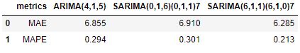
- Calculating the MAE and MAPE metrics and printing the summary
from sklearn.metrics import mean_absolute_error, mean_absolute_percentage_error

metrics_arima = [round(mean_absolute_error(df_store_2_item_28_time[-90:],arima_mean),3),
                 round(mean_absolute_percentage_error(df_store_2_item_28_time[-90:],arima_mean),3)]
metrics_sarima_01 = [round(mean_absolute_error(df_store_2_item_28_time[-90:],sarima_01_mean),3),
                       round(mean_absolute_percentage_error(df_store_2_item_28_time[-90:],sarima_01_mean),3)]
metrics_sarima_02 = [round(mean_absolute_error(df_store_2_item_28_time[-90:],sarima_02_mean),3),
                       round(mean_absolute_percentage_error(df_store_2_item_28_time[-90:],sarima_02_mean),3)]
df_arima_results = pd.DataFrame({'metrics':['MAE','MAPE'],
              'ARIMA(4,1,5)':metrics_arima,
              'SARIMA(0,1,6)(0,1,1)7':metrics_sarima_01,
              'SARIMA(6,1,1)(6,1,0)7':metrics_sarima_02,
             })

df_arima_results

metrics	ARIMA(4,1,5)	SARIMA(0,1,6)(0,1,1)7	SARIMA(6,1,1)(6,1,0)7
0	MAE	6.855	6.910	6.285
1	MAPE	0.294	0.301	0.213
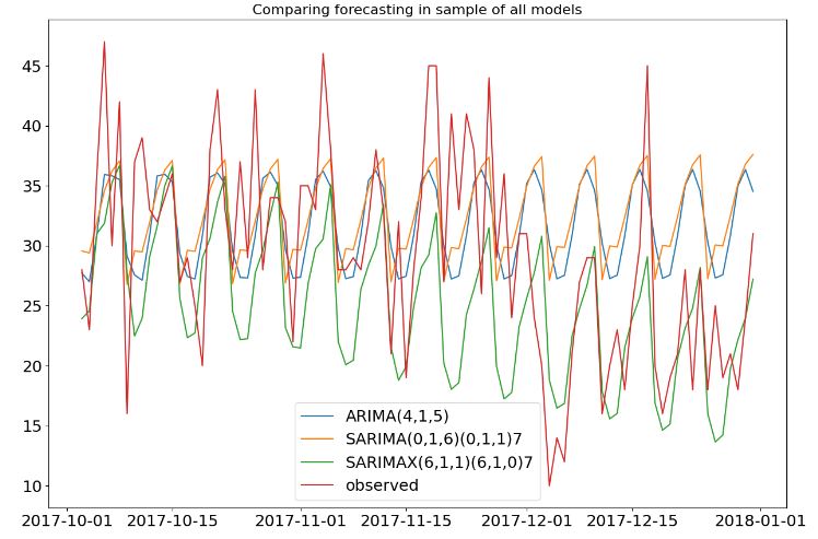
- Comparing forecasting in sample of all models
dates = df_store_2_item_28_time.index
# Plot mean ARIMA and SARIMA predictions and observed
plt.figure(figsize=(15,10))
plt.title('Comparing forecasting in sample of all models', size = 16)
plt.plot(arima_mean.index, arima_mean, label='ARIMA(4,1,5)')
plt.plot(sarima_01_mean.index, sarima_01_mean, label='SARIMA(0,1,6)(0,1,1)7')
plt.plot(sarima_02_mean.index, sarima_02_mean, label='SARIMAX(6,1,1)(6,1,0)7')
plt.plot(df_store_2_item_28_time[-90:], label='observed')
plt.legend()
plt.show()
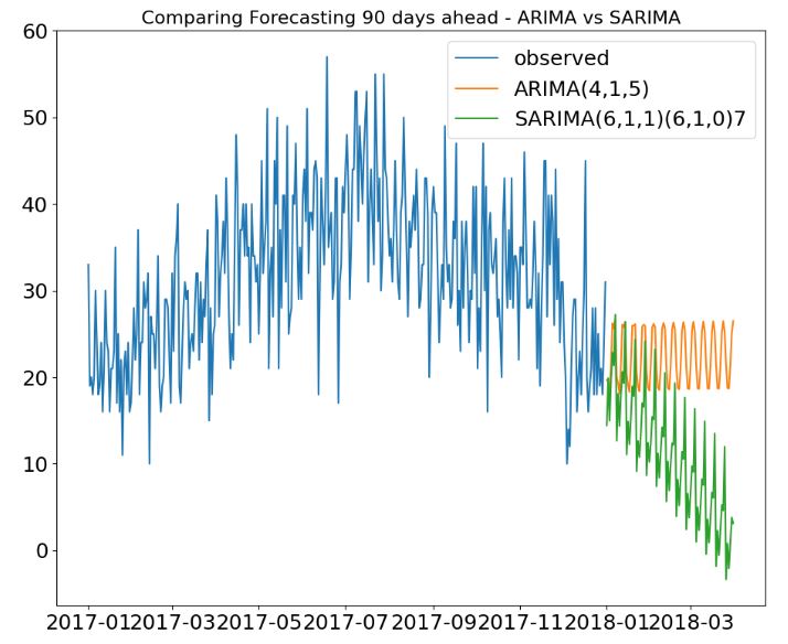
- Comparing Forecasting 90 days ahead – ARIMA vs SARIMA
#Forecast Out of Sample
# Create ARIMA mean forecast
arima_pred = arima_results.get_forecast(steps=90)
arima_mean = arima_pred.predicted_mean
# Create SARIMA mean forecast
sarima_02_pred = sarima_02_results.get_forecast(steps=90)
sarima_02_mean = sarima_02_pred.predicted_mean
dates = df_store_2_item_28_time.index
# Plot mean ARIMA and SARIMA predictions and observed
plt.title("Comparing Forecasting 90 days ahead - ARIMA vs SARIMA", size =16)
plt.plot(df_store_2_item_28_time['2017':], label='observed')
plt.plot(arima_mean.index, arima_mean, label='ARIMA(4,1,5)')
plt.plot(sarima_02_mean.index, sarima_02_mean, label='SARIMA(6,1,1)(6,1,0)7')
plt.legend()
plt.show()
Summary
- We compared 3 optimized FB Prophet models to forecast sales at the store level with high seasonality effects. The final model Prophet_03 yields MAE=4.252 and MAPE=0.168.
- Referring to these models, our observations support the following 2 aspects of previous case studies: (1) a native handling of trend and seasonality features, that makes FB Prophet a good baseline model if the time series follows sales cycles; (2) if your signal is noisy, fine-tuning the model’s performance can be a hassle.
- We also considered various autoregressive (AR) models. Specifically, SARIMAX models are among the most widely used AR models for forecasting, with good forecasting performance. In the SARIMAX model notation, the parameters p , d , and q represent the autoregressive, differencing, and moving-average components, respectively.
- We studied possible combinations of AR models for different values of (p , d , q). As a result of hyperparameter optimization, we calculated MAE and MAPE for the following 3 AR models: AR1=ARIMA(4,1,5), AR2=SARIMA(0,1,6)(0,1,1)7, and AR3=SARIMA(6,1,1)(6,1,0)7. AR3 is the the final AR model with MAE=6.285 and MAPE=0.213.
- If we look at the residual time-series plot, there is no trend or seasonal pattern, so it can be assumed that the residuals are normally distributed. This is also supported by the model residual histogram, which is bell-shaped, meaning the residuals are normally distributed.
- Event though SARIMA models allow for differencing data by seasonal frequency, FB Prophet provides an interpretable model with the best (short-time) performance.
- This data can also be applied to more complex forecasting models or by combining other forecasting methods to increase the accuracy of forecasting results.
- Business impact: if there is a significant decline in sales, then we can identify promotional strategies that have least impact on sales and further boost profitable promotional strategies.
Explore More
- Leveraging Predictive Uncertainties of Time Series Forecasting Models
- Evaluation of ML Sales Forecasting: tslearn, Random Walk, Holt-Winters, SARIMAX, GARCH, Prophet, and LSTM
- A Balanced Mix-and-Match Time Series Forecasting: ThymeBoost, Prophet, and AutoARIMA
- Low-Code AutoEDA of Dutch eHealth Data in Python
- A Comparison of Automated EDA Tools in Python: Pandas-Profiling vs SweetViz
- Time Series Forecasting of Hourly U.S.A. Energy Consumption – PJM East Electricity Grid
- SARIMAX Cross-Validation of EIA Crude Oil Prices Forecast in 2023 – 2. Brent
- SARIMAX-TSA Forecasting, QC and Visualization of Online Food Delivery Sales
- BTC-USD Freefall vs FB/Meta Prophet 2022-23 Predictions
- Stock Forecasting with FBProphet
- Brazilian E-Commerce Showcase
- Unsupervised ML Clustering, Customer Segmentation, Cohort, Market Basket, Bank Churn, CRM, ABC & RFM Analysis – A Comprehensive Guide in Python
References
- Time Series Part 3: Forecasting with Facebook Prophet: An Intro
- Time Series Part 2: Forecasting with SARIMAX models: An Intro
- Prophet vs SARIMA — Time Series Forecasting
- MKB-DataLab
- Time Series Model (SARIMAX Vs LSTM Vs fbprophet)
- An End-to-End Project on Time Series Analysis and Forecasting with Python
- ARIMA for Time-Series Forecasting: Retail Sales Predictions


One-Time
Monthly
Yearly
Make a one-time donation
Make a monthly donation
Make a yearly donation
Choose an amount
€5.00
€15.00
€100.00
€5.00
€15.00
€100.00
€5.00
€15.00
€100.00
Or enter a custom amount
€
Your contribution is appreciated.
Your contribution is appreciated.
Your contribution is appreciated.
DonateDonate monthlyDonate yearly
Leave a comment