
Contents:
- Introduction
- Importing Libraries
- Input Data
- Exploratory Data Analysis
- Data Preparation & Pre-Processing
- Model Training, Testing and Validation
- Output Data
- Summary Report
- Conclusions


How to Improve Customer Retention & Generate Revenue With Your CX Programme.
Introduction
Customer churn rate is the percentage of customers that sign up and then leave within a given amount of time. Whereas customer retention rate is the percentage of customers that sign up and stay with you.
To put it simply, churn rate is bad because it means you’re losing customers, and retention rate is good because it means you’re keeping customers.
There are three major benefits to having a high customer retention rate and a low customer churn rate:
- you’re likely spending money on new customer acquisition costs
- a low churn rate and high retention rate means your customers are happy with your product
- having a high retention rate allows you to accurately predict your future revenue.
The simplest way to calculate your customer churn rate is to use the basic churn calculation of:
Number of customers who left / total number of customers x 100
For example, if you had 1000 new customers in a given time period and 50 of them left without renewing their subscription, you would have a churn rate of 5%. Because 50 divided by 1000 is 0.05; multiply that by 100 and you get 5%.
Just like user retention rate, you’ll want to calculate your churn rate on a monthly, quarterly, and/or annual basis depending on how long your subscription agreements last for.
The objective of this project is to build a Machine Learning (ML) Python model to predict, with reasonable accuracy, those customers who are going to churn soon. In doing so, we need to install the Anaconda IDE with the Jupyter Notebook and all relevant ML libraries.
Importing Libraries
!pip install joblib lightgbm matplotlib numpy pandas scikit_learn seaborn xgboost
import pandas as pd
import numpy as np
import matplotlib.pyplot as plt
import seaborn as sns
from sklearn.preprocessing import LabelEncoder, OneHotEncoder, StandardScaler
from sklearn.feature_selection import RFE
from sklearn.linear_model import LogisticRegression
from sklearn.svm import SVC
from sklearn.decomposition import PCA
from sklearn.tree import DecisionTreeClassifier, export_graphviz
from sklearn.pipeline import Pipeline
from sklearn.model_selection import train_test_split
from lightgbm import LGBMClassifier
from sklearn.metrics import roc_auc_score, recall_score, confusion_matrix, classification_report
import subprocess
import joblib
Get multiple outputs in the same cell
from IPython.core.interactiveshell import InteractiveShell
InteractiveShell.ast_node_interactivity = “all”
Ignore all warnings
import warnings
warnings.filterwarnings(‘ignore’)
warnings.filterwarnings(action=’ignore’, category=DeprecationWarning)
pd.set_option(‘display.max_columns’, None)
pd.set_option(‘display.max_rows’, None)
Input Data
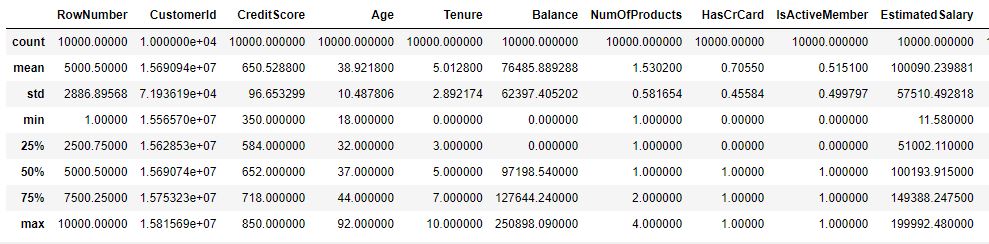
The Kaggle churn modelling dataset consists of 10000 rows representing a customer and 15 columns: 14 features and 1 target feature, Exited = whether the customer churned or not. The data consists of both numerical and categorical features:
CustomerId: A unique ID of the customer.CreditScore: The credit score of the customer,Age: The age of the customer,Tenure: The number of months the client has been with the firm.Balance: Balance remaining in the customer account,NumOfProducts: The number of products sold by the customer.EstimatedSalary: The estimated salary of the customer.
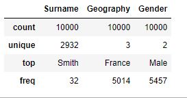
Surname: The surname of the customer.Geography: The country of the customer.Gender: M/FHasCrCard: Whether the customer has a credit card or not.IsActiveMember: Whether the customer is active or not.
Reading the dataset
dc = pd.read_csv(“YourPath/Churn_Modelling.csv”)
dc.head(5)

Exploratory Data Analysis
Dimension of the dataset
dc.shape
(10000, 14)
Describe all numerical columns
dc.describe(exclude= [‘O’])
Describe all categorical columns
dc.describe(include = [‘O’])
Checking number of unique customers in the dataset
dc.shape[0], dc.CustomerId.nunique()
(10000, 10000)
Churn Value Distribution
dc[“Exited”].value_counts()
0    7963
1    2037
Name: Exited, dtype: int64
dc.groupby([‘Surname’]).agg({‘RowNumber’:’count’, ‘Exited’:’mean’}
).reset_index().sort_values(by=’RowNumber’, ascending=False).head()

dc.groupby([‘Geography’]).agg({‘RowNumber’:’count’, ‘Exited’:’mean’}
).reset_index().sort_values(by=’RowNumber’, ascending=False)

sns.set(style=”whitegrid”)
sns.boxplot(y=dc[‘CreditScore’])

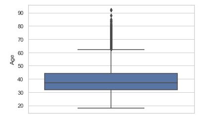
sns.boxplot(y=dc[‘Age’])
sns.violinplot(y = dc.Tenure)

sns.violinplot(y = dc[‘Balance’])

sns.set(style = ‘ticks’)
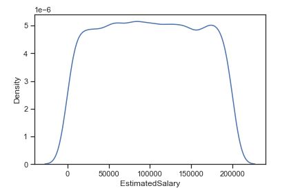
sns.distplot(dc.NumOfProducts, hist=True, kde=False)

When dealing with numerical characteristics, one of the most useful statistics to examine is the data distribution. We can use Kernel-Density-Estimation plot for that purpose.
Data Preparation & Pre-Processing
Separating out different columns into various categories as defined below:
target_var = [‘Exited’]
cols_to_remove = [‘RowNumber’, ‘CustomerId’]
numerical columns
num_feats = [‘CreditScore’, ‘Age’, ‘Tenure’, ‘Balance’, ‘NumOfProducts’, ‘EstimatedSalary’]
and categorical columns
cat_feats = [‘Surname’, ‘Geography’, ‘Gender’, ‘HasCrCard’, ‘IsActiveMember’]
Get values of target_var and drop redundant columns cols_to_remove
y = dc[target_var].values
dc.drop(cols_to_remove, axis=1, inplace=True)
Keeping aside a test/holdout set
dc_train_val, dc_test, y_train_val, y_test = train_test_split(dc, y.ravel(), test_size = 0.1, random_state = 42)
Splitting data into train and validation sets
dc_train, dc_val, y_train, y_val = train_test_split(dc_train_val, y_train_val, test_size = 0.12, random_state = 42)
dc_train.shape, dc_val.shape, dc_test.shape, y_train.shape, y_val.shape, y_test.shape
np.mean(y_train), np.mean(y_val), np.mean(y_test)
((7920, 12), (1080, 12), (1000, 12), (7920,), (1080,), (1000,))
(0.20303030303030303, 0.22037037037037038, 0.191)
Label encoding with the sklearn method
le = LabelEncoder()
Label encoding of the Gender variable
dc_train[‘Gender’] = le.fit_transform(dc_train[‘Gender’])
le_gender_mapping = dict(zip(le.classes_, le.transform(le.classes_)))
le_gender_mapping
{'Female': 0, 'Male': 1}
Encoding Gender feature for validation and test sets
dc_val[‘Gender’] = dc_val.Gender.map(le_gender_mapping)
dc_test[‘Gender’] = dc_test.Gender.map(le_gender_mapping)
Filling missing/NaN values created due to new categorical levels
dc_val[‘Gender’].fillna(-1, inplace=True)
dc_test[‘Gender’].fillna(-1, inplace=True)
dc_train.Gender.unique(), dc_val.Gender.unique(), dc_test.Gender.unique()
(array([1, 0]), array([1, 0]), array([1, 0]))
Encoding with the sklearn method(LabelEncoder())
le_ohe = LabelEncoder()
ohe = OneHotEncoder(handle_unknown = ‘ignore’, sparse=False)
enc_train = le_ohe.fit_transform(dc_train.Geography).reshape(dc_train.shape[0],1)
ohe_train = ohe.fit_transform(enc_train)
ohe_train
array([[0., 1., 0.],
       [1., 0., 0.],
       [1., 0., 0.],
       ...,
       [1., 0., 0.],
       [0., 1., 0.],
       [0., 1., 0.]])
Geography mapping between classes
le_ohe_geography_mapping = dict(zip(le_ohe.classes_, le_ohe.transform(le_ohe.classes_)))
le_ohe_geography_mapping
{'France': 0, 'Germany': 1, 'Spain': 2}
Encoding Geography feature for validation and test set
enc_val = dc_val.Geography.map(le_ohe_geography_mapping).ravel().reshape(-1,1)
enc_test = dc_test.Geography.map(le_ohe_geography_mapping).ravel().reshape(-1,1)
Filling missing/NaN values created due to new categorical levels
enc_val[np.isnan(enc_val)] = 9999
enc_test[np.isnan(enc_test)] = 9999
and apply transform
ohe_val = ohe.transform(enc_val)
ohe_test = ohe.transform(enc_test)
See what happens when a new value is encapsulated into the ohe
ohe.transform(np.array([[9999]]))
array([[0., 0., 0.]])
cols = [‘country_’ + str(x) for x in le_ohe_geography_mapping.keys()]
cols
['country_France', 'country_Germany', 'country_Spain']
Adding to the respective dataframes
dc_train = pd.concat([dc_train.reset_index(), pd.DataFrame(ohe_train, columns = cols)], axis = 1).drop([‘index’], axis=1)
dc_val = pd.concat([dc_val.reset_index(), pd.DataFrame(ohe_val, columns = cols)], axis = 1).drop([‘index’], axis=1)
dc_test = pd.concat([dc_test.reset_index(), pd.DataFrame(ohe_test, columns = cols)], axis = 1).drop([‘index’], axis=1)
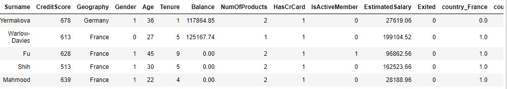
print(“Training set”)
dc_train.head()
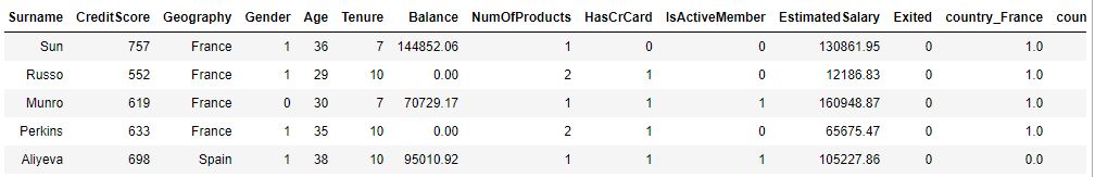
print(“\n\nValidation set”)
dc_val.head()
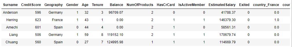
print(“\n\nTest set”)
dc_test.head()
Training set
Validation set
Test set
Let’s apply drop, group and global mean
dc_train.drop([‘Geography’], axis=1, inplace=True)
dc_val.drop([‘Geography’], axis=1, inplace=True)
dc_test.drop([‘Geography’], axis=1, inplace=True)
means = dc_train.groupby([‘Surname’]).Exited.mean()
means.head()
means.tail()
Surname
Abazu       0.00
Abbie       0.00
Abbott      0.25
Abdullah    1.00
Abdulov     0.00
Name: Exited, dtype: float64
Surname
Zubarev     0.0
Zubareva    0.0
Zuev        0.0
Zuyev       0.0
Zuyeva      0.0
Name: Exited, dtype: float64
global_mean = y_train.mean()
global_mean
0.20303030303030303
Creating new encoded features for surname – Target (mean) encoding and group
dc_train[‘Surname_mean_churn’] = dc_train.Surname.map(means)
dc_train[‘Surname_mean_churn’].fillna(global_mean, inplace=True)
freqs = dc_train.groupby([‘Surname’]).size()
freqs.head()
Surname
Abazu       2
Abbie       1
Abbott      4
Abdullah    1
Abdulov     1
dtype: int64
dc_train[‘Surname_freq’] = dc_train.Surname.map(freqs)
dc_train[‘Surname_freq’].fillna(0, inplace=True)
dc_train[‘Surname_enc’] = ((dc_train.Surname_freq * dc_train.Surname_mean_churn) – dc_train.Exited)/(dc_train.Surname_freq – 1)
Fill NaNs occuring due to category frequency being 1 or less
dc_train[‘Surname_enc’].fillna((((dc_train.shape[0] * global_mean) – dc_train.Exited) / (dc_train.shape[0] – 1)), inplace=True)
dc_train.head(5)

Replacing by category means and new category levels by global mean
dc_val[‘Surname_enc’] = dc_val.Surname.map(means)
dc_val[‘Surname_enc’].fillna(global_mean, inplace=True)
dc_test[‘Surname_enc’] = dc_test.Surname.map(means)
dc_test[‘Surname_enc’].fillna(global_mean, inplace=True)
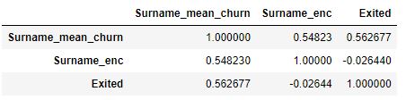
Show that using Target encoding decorrelates features
dc_train[[‘Surname_mean_churn’, ‘Surname_enc’, ‘Exited’]].corr()
dc_train.drop([‘Surname_mean_churn’], axis=1, inplace=True)
dc_train.drop([‘Surname_freq’], axis=1, inplace=True)
dc_train.drop([‘Surname’], axis=1, inplace=True)
dc_val.drop([‘Surname’], axis=1, inplace=True)
dc_test.drop([‘Surname’], axis=1, inplace=True)
dc_train.head()

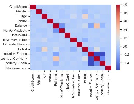
Let’s calculate the feature correlation matrix
corr = dc_train.corr()
sns.heatmap(corr, cmap = ‘coolwarm’)
sns.boxplot(x=”Exited”, y=”Age”, data=dc_train, palette=”Set3″)

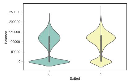
sns.violinplot(x=”Exited”, y=”Balance”, data=dc_train, palette=”Set3″)
Check key groups
cat_vars_bv = [‘Gender’, ‘IsActiveMember’, ‘country_Germany’, ‘country_France’]
for col in cat_vars_bv:
dc_train.groupby([col]).Exited.mean()
print()
Gender
0    0.248191
1    0.165511
Name: Exited, dtype: float64
IsActiveMember
0    0.266285
1    0.143557
Name: Exited, dtype: float64
country_Germany
0.0    0.163091
1.0    0.324974
Name: Exited, dtype: float64
country_France
0.0    0.245877
1.0    0.160593
Name: Exited, dtype: float64
Computed mean on churned or non chuned custmers group by number of product on training data
NumOfProducts
1    0.273428
2    0.076881
3    0.825112
4    1.000000
Name: Exited, dtype: float64
1    4023
2    3629
3     223
4      45
Name: NumOfProducts, dtype: int64
Add small regualrization parameter
eps = 1e-6
dc_train[‘bal_per_product’] = dc_train.Balance/(dc_train.NumOfProducts + eps)
dc_train[‘bal_by_est_salary’] = dc_train.Balance/(dc_train.EstimatedSalary + eps)
dc_train[‘tenure_age_ratio’] = dc_train.Tenure/(dc_train.Age + eps)
dc_train[‘age_surname_mean_churn’] = np.sqrt(dc_train.Age) * dc_train.Surname_enc
Create the list of columns
new_cols = [‘bal_per_product’, ‘bal_by_est_salary’, ‘tenure_age_ratio’, ‘age_surname_mean_churn’]
Check that the new column doesn’t have any missing values
bal_per_product           0
bal_by_est_salary         0
tenure_age_ratio          0
age_surname_mean_churn    0
dtype: int64
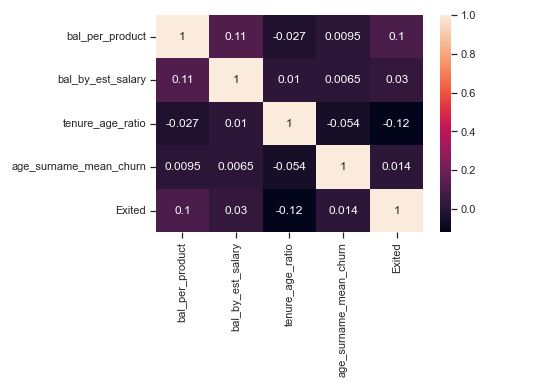
Compute correlations of new columns with target variables to judge their importance
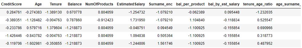
Let’s apply scaling/normalization of the above columns
dc_val[‘bal_per_product’] = dc_val.Balance/(dc_val.NumOfProducts + eps)
dc_val[‘bal_by_est_salary’] = dc_val.Balance/(dc_val.EstimatedSalary + eps)
dc_val[‘tenure_age_ratio’] = dc_val.Tenure/(dc_val.Age + eps)
dc_val[‘age_surname_mean_churn’] = np.sqrt(dc_val.Age) * dc_val.Surname_enc
dc_test[‘bal_per_product’] = dc_test.Balance/(dc_test.NumOfProducts + eps)
dc_test[‘bal_by_est_salary’] = dc_test.Balance/(dc_test.EstimatedSalary + eps)
dc_test[‘tenure_age_ratio’] = dc_test.Tenure/(dc_test.Age + eps)
dc_test[‘age_surname_mean_churn’] = np.sqrt(dc_test.Age) * dc_test.Surname_enc
Let’s initialize the standard scaler
sc = StandardScaler()
cont_vars = [‘CreditScore’, ‘Age’, ‘Tenure’, ‘Balance’, ‘NumOfProducts’, ‘EstimatedSalary’, ‘Surname_enc’, ‘bal_per_product’
, ‘bal_by_est_salary’, ‘tenure_age_ratio’, ‘age_surname_mean_churn’]
cat_vars = [‘Gender’, ‘HasCrCard’, ‘IsActiveMember’, ‘country_France’, ‘country_Germany’, ‘country_Spain’]
Scaling only continuous columns
cols_to_scale = cont_vars
sc_X_train = sc.fit_transform(dc_train[cols_to_scale])
Converting from array to dataframe and naming the respective features/columns
sc_X_train = pd.DataFrame(data=sc_X_train, columns=cols_to_scale)
sc_X_train.shape
sc_X_train.head()
(7920, 11)
Scaling validation and test sets by transforming the mapping obtained through the training set
sc_X_val = sc.transform(dc_val[cols_to_scale])
sc_X_test = sc.transform(dc_test[cols_to_scale])
Converting val and test arrays to dataframes for re-usability
sc_X_val = pd.DataFrame(data=sc_X_val, columns=cols_to_scale)
sc_X_test = pd.DataFrame(data=sc_X_test, columns=cols_to_scale)
Creating feature-set and target for RFE model
y = dc_train[‘Exited’].values
X = dc_train[cat_vars + cont_vars]
X.columns = cat_vars + cont_vars
X.columns
Index(['Gender', 'HasCrCard', 'IsActiveMember', 'country_France',
       'country_Germany', 'country_Spain', 'CreditScore', 'Age', 'Tenure',
       'Balance', 'NumOfProducts', 'EstimatedSalary', 'Surname_enc',
       'bal_per_product', 'bal_by_est_salary', 'tenure_age_ratio',
       'age_surname_mean_churn'],
      dtype='object')
Model Training, Testing and Validation
Preparations for logistics regression
rfe = RFE(estimator=LogisticRegression(), n_features_to_select=10)
rfe = rfe.fit(X.values, y)
Masking of selected features and the feature ranking, such that ranking_[i] corresponds to the ranking position of the i-th feature
print(rfe.support_)
print(rfe.ranking_)
[ True  True  True  True  True  True False  True False False  True False
  True False False  True False]
[1 1 1 1 1 1 4 1 3 6 1 8 1 7 5 1 2]
Let’s apply linear logistic regression
mask = rfe.support_.tolist()
selected_feats = [b for a,b in zip(mask, X.columns) if a]
selected_feats
['Gender',
 'HasCrCard',
 'IsActiveMember',
 'country_France',
 'country_Germany',
 'country_Spain',
 'Age',
 'NumOfProducts',
 'Surname_enc',
 'tenure_age_ratio']
rfe_dt = RFE(estimator=DecisionTreeClassifier(max_depth = 4, criterion = ‘entropy’), n_features_to_select=10)
rfe_dt = rfe_dt.fit(X.values, y)
mask = rfe_dt.support_.tolist()
selected_feats_dt = [b for a,b in zip(mask, X.columns) if a]
selected_feats_dt
['IsActiveMember',
 'country_Germany',
 'Age',
 'NumOfProducts',
 'EstimatedSalary',
 'Surname_enc',
 'bal_per_product',
 'bal_by_est_salary',
 'tenure_age_ratio',
 'age_surname_mean_churn']
selected_cat_vars = [x for x in selected_feats if x in cat_vars]
selected_cont_vars = [x for x in selected_feats if x in cont_vars]
Using categorical features and scaled numerical features
X_train = np.concatenate((dc_train[selected_cat_vars].values, sc_X_train[selected_cont_vars].values), axis=1)
X_val = np.concatenate((dc_val[selected_cat_vars].values, sc_X_val[selected_cont_vars].values), axis=1)
X_test = np.concatenate((dc_test[selected_cat_vars].values, sc_X_test[selected_cont_vars].values), axis=1)
Print the shapes of training, validation and test sets
X_train.shape, X_val.shape, X_test.shape
((7920, 10), (1080, 10), (1000, 10))
Obtaining class weights based on the class samples imbalance ratio
_, num_samples = np.unique(y_train, return_counts=True)
weights = np.max(num_samples)/num_samples
Define the weight dictionary
weights_dict = dict()
class_labels = [0,1]
Define weights associated with classes
for a,b in zip(class_labels,weights):
weights_dict[a] = b
weights_dict
{0: 1.0, 1: 3.925373134328358}
Defining model
lr = LogisticRegression(C=1.0, penalty=’l2′, class_weight=weights_dict, n_jobs=-1)
Training
lr.fit(X_train, y_train)
print(f’Confusion Matrix: \n{confusion_matrix(y_val, lr.predict(X_val))}’)
print(f’Area Under Curve: {roc_auc_score(y_val, lr.predict(X_val))}’)
print(f’Recall score: {recall_score(y_val,lr.predict(X_val))}’)
print(f’Classification report: \n{classification_report(y_val,lr.predict(X_val))}’)
LogisticRegression(class_weight={0: 1.0, 1: 3.925373134328358}, n_jobs=-1)
Confusion Matrix:
[[590 252]
 [ 71 167]]
Area Under Curve: 0.7011966306712709
Recall score: 0.7016806722689075
Classification report:
              precision    recall  f1-score   support

           0       0.89      0.70      0.79       842
           1       0.40      0.70      0.51       238

    accuracy                           0.70      1080
   macro avg       0.65      0.70      0.65      1080
weighted avg       0.78      0.70      0.72      1080
Define the SVM linear kernel
svm = SVC(C=1.0, kernel=”linear”, class_weight=weights_dict)
svm.fit(X_train, y_train)
SVC(class_weight={0: 1.0, 1: 3.925373134328358}, kernel='linear')
Validation metrics
print(f’Confusion Matrix: {confusion_matrix(y_val, lr.predict(X_val))}’)
print(f’Area Under Curve: {roc_auc_score(y_val, lr.predict(X_val))}’)
print(f’Recall score: {recall_score(y_val,lr.predict(X_val))}’)
print(f’Classification report: \n{classification_report(y_val,lr.predict(X_val))}’)
Confusion Matrix: [[590 252]
 [ 71 167]]
Area Under Curve: 0.7011966306712709
Recall score: 0.7016806722689075
Classification report:
              precision    recall  f1-score   support

           0       0.89      0.70      0.79       842
           1       0.40      0.70      0.51       238

    accuracy                           0.70      1080
   macro avg       0.65      0.70      0.65      1080
weighted avg       0.78      0.70      0.72      1080
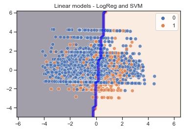
Let’s apply PCA
pca = PCA(n_components=2)
Transforming the dataset using PCA
X_pca = pca.fit_transform(X_train)
y = y_train
X_pca.shape, y.shape
((7920, 2), (7920,))
Get min and max values
xmin, xmax = X_pca[:, 0].min() – 2, X_pca[:, 0].max() + 2
ymin, ymax = X_pca[:, 1].min() – 2, X_pca[:, 1].max() + 2
Creating a mesh region where the boundary will be plotted
xx, yy = np.meshgrid(np.arange(xmin, xmax, 0.2),
np.arange(ymin, ymax, 0.2))
Fitting LR model on 2 features
lr.fit(X_pca, y)
Fitting SVM model on 2 features
svm.fit(X_pca, y)
Plotting decision boundary for LR
z1 = lr.predict(np.c_[xx.ravel(), yy.ravel()])
z1 = z1.reshape(xx.shape)
Plotting decision boundary for SVM
z2 = svm.predict(np.c_[xx.ravel(), yy.ravel()])
z2 = z2.reshape(xx.shape)
Displaying the result
plt.contourf(xx, yy, z1, alpha=0.4) # LR
plt.contour(xx, yy, z2, alpha=0.4, colors=’blue’) # SVM
sns.scatterplot(X_pca[:,0], X_pca[:,1], hue=y_train, s=50, alpha=0.8)
plt.title(‘Linear models – LogReg and SVM’)
LogisticRegression(class_weight={0: 1.0, 1: 3.925373134328358}, n_jobs=-1)
Out[89]:
SVC(class_weight={0: 1.0, 1: 3.925373134328358}, kernel='linear')
Out[89]:
<matplotlib.contour.QuadContourSet at 0x214420110a0>
Out[89]:
<matplotlib.contour.QuadContourSet at 0x21442019c10>
Out[89]:
<AxesSubplot:>
Out[89]:
Text(0.5, 1.0, 'Linear models - LogReg and SVM')
Features selected from the RFE process
selected_feats_dt
['IsActiveMember',
 'country_Germany',
 'Age',
 'NumOfProducts',
 'EstimatedSalary',
 'Surname_enc',
 'bal_per_product',
 'bal_by_est_salary',
 'tenure_age_ratio',
 'age_surname_mean_churn']
Re-defining X_train and X_val to consider original unscaled continuous features. y_train and y_val remain unaffected
X_train = dc_train[selected_feats_dt].values
X_val = dc_val[selected_feats_dt].values
Decision tree classiier model
clf = DecisionTreeClassifier(criterion=’entropy’, class_weight=weights_dict, max_depth=4, max_features=None
, min_samples_split=25, min_samples_leaf=15)
Fit the model
clf.fit(X_train, y_train)
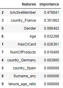
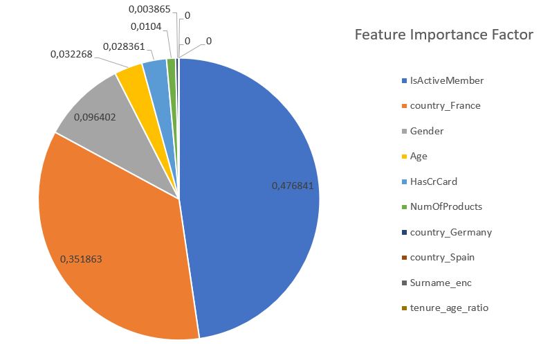
Checking the importance of different features of the model
pd.DataFrame({‘features’: selected_feats,
‘importance’: clf.feature_importances_
}).sort_values(by=’importance’, ascending=False)
DecisionTreeClassifier(class_weight={0: 1.0, 1: 3.925373134328358},
                       criterion='entropy', max_depth=4, min_samples_leaf=15,
                       min_samples_split=25)
Validation metrics
print(f’Confusion Matrix: {confusion_matrix(y_val, clf.predict(X_val))}’)
print(f’Area Under Curve: {roc_auc_score(y_val, clf.predict(X_val))}’)
print(f’Recall score: {recall_score(y_val,clf.predict(X_val))}’)
print(f’Classification report: \n{classification_report(y_val,clf.predict(X_val))}’)
Confusion Matrix: [[633 209]
 [ 61 177]]
Area Under Curve: 0.7477394758378411
Recall score: 0.7436974789915967
Classification report:
              precision    recall  f1-score   support

           0       0.91      0.75      0.82       842
           1       0.46      0.74      0.57       238

    accuracy                           0.75      1080
   macro avg       0.69      0.75      0.70      1080
weighted avg       0.81      0.75      0.77      1080
Decision Tree Classifier
clf = DecisionTreeClassifier(criterion=’entropy’, class_weight=weights_dict,
max_depth=3, max_features=None,
min_samples_split=25, min_samples_leaf=15)
We fit the model
clf.fit(X_train, y_train)
DecisionTreeClassifier(class_weight={0: 1.0, 1: 3.925373134328358},
                       criterion='entropy', max_depth=3, min_samples_leaf=15,
                       min_samples_split=25)
Export now as a dot file
dot_data = export_graphviz(clf, out_file=’tree.dot’,
feature_names=selected_feats_dt,
class_names=[‘Did not churn’, ‘Churned’],
rounded=True, proportion=False,
precision=2, filled=True)
!pip install utils
Collecting utils
  Using cached utils-1.0.1-py2.py3-none-any.whl (21 kB)
Installing collected packages: utils
Successfully installed utils-1.0.1
model = clf.fit(X_train, y_train)
X_test = dc_test.drop(columns=[‘Exited’], axis=1)
Predict target probabilities
test_probs = model.predict_proba(X_test)[:,1]
Predict target values on test data
test_preds = np.where(test_probs > 0.45, 1, 0)
with the flexibility to tweak the probability threshold
0.7043793967084955
Out[112]:
0.6596858638743456
Out[112]:
array([[606, 203],
       [ 65, 126]], dtype=int64)
              precision    recall  f1-score   support

           0       0.90      0.75      0.82       809
           1       0.38      0.66      0.48       191

    accuracy                           0.73      1000
   macro avg       0.64      0.70      0.65      1000
weighted avg       0.80      0.73      0.76      1000
Adding predictions and their probabilities in the original test dataframe
test = dc_test.copy()
test[‘predictions’] = test_preds
test[‘pred_probabilities’] = test_probs
test.sample(5)

high_churn_list = test[test.pred_probabilities > 0.7].sort_values(by=[‘pred_probabilities’], ascending=False
).reset_index().drop(columns=[‘index’, ‘Exited’, ‘predictions’], axis=1)
high_churn_list.shape
high_churn_list.head()

Output Data
Save the output model data
high_churn_list.to_csv(‘YOURPATH/high_churn_list.csv’, index=False)
Summary Report
Training Data:
LogisticRegression(class_weight={0: 1.0, 1: 3.925373134328358}, n_jobs=-1)
Confusion Matrix:
[[590 252]
 [ 71 167]]
Area Under Curve: 0.7011966306712709
Recall score: 0.7016806722689075
Classification report:
              precision    recall  f1-score   support

           0       0.89      0.70      0.79       842
           1       0.40      0.70      0.51       238

    accuracy                           0.70      1080
   macro avg       0.65      0.70      0.65      1080
weighted avg       0.78      0.70      0.72      1080
SVC(class_weight={0: 1.0, 1: 3.925373134328358}, kernel='linear')
Confusion Matrix: [[590 252]
 [ 71 167]]
Area Under Curve: 0.7011966306712709
Recall score: 0.7016806722689075
Classification report:
              precision    recall  f1-score   support

           0       0.89      0.70      0.79       842
           1       0.40      0.70      0.51       238

    accuracy                           0.70      1080
   macro avg       0.65      0.70      0.65      1080
weighted avg       0.78      0.70      0.72      1080
DecisionTreeClassifier(class_weight={0: 1.0, 1: 3.925373134328358},
                       criterion='entropy', max_depth=4, min_samples_leaf=15,
                       min_samples_split=25)
Confusion Matrix: [[633 209]
 [ 61 177]]
Area Under Curve: 0.7477394758378411
Recall score: 0.7436974789915967
Classification report:
              precision    recall  f1-score   support

           0       0.91      0.75      0.82       842
           1       0.46      0.74      0.57       238

    accuracy                           0.75      1080
   macro avg       0.69      0.75      0.70      1080
weighted avg       0.81      0.75      0.77      1080
Test set metrics
roc_auc_score(y_test, test_preds)
recall_score(y_test, test_preds)
confusion_matrix(y_test, test_preds)
print(classification_report(y_test, test_preds))
0.7043793967084955
Out[112]:
0.6596858638743456
Out[112]:
array([[606, 203],
       [ 65, 126]], dtype=int64)
              precision    recall  f1-score   support

           0       0.90      0.75      0.82       809
           1       0.38      0.66      0.48       191

    accuracy                           0.73      1000
   macro avg       0.64      0.70      0.65      1000
weighted avg       0.80      0.73      0.76      1000
Conclusions
Churn rate is a critical metric of customer satisfaction. Low churn rates mean happy customers; high churn rates mean customers are leaving you. A small rate of monthly/quarterly churn compounds over time. 1% monthly churn quickly translates to almost 12% yearly churn.
According to Forbes, it takes a lot more money (up to five times more) to get new customers than to keep the ones you already have. Churn tells you how many existing customers are leaving your business, so lowering churn has a big positive impact on your revenue streams.
Churn is a good indicator of growth potential. Churn rates track lost customers, and growth rates track new customers—comparing and analyzing both of these metrics tells you exactly how much your business is growing over time. If growth is higher than churn, you can say your business is growing. If churn is higher than growth, your business is getting smaller.
In this project, we explored the churn rate in-depth and examined an example implementation of a ML/AI churn rate prediction system.


Leave a comment