
Cohort Analysis in E-Commerce Marketing
Cohort analysis (CA) is a method by which you can monitor the overall health of your marketing campaigns in terms of the customer retention rate. CA offers a unique opportunity to judge the efficiency of marketing efforts. It can also enlighten marketers as to which cohorts (i.e. groups of customers and/or contacts) are the most valuable to your brand. Here are a few good examples:
- How long does it take subscribers to become customers?
- How long does it take for a customer to return?
- Is each stage of the customer lifecycle being nurtured effectively?
- What are the long-term purchasing habits of different demographic segments?
- Which channels are driving the best results?
- Do I have many seasonal shoppers?
- Are those subscribed spending more than those unsubscribed?
- Different stores, different results?
Bottom line: CA is the gift that keeps on giving.
Customer Transaction Showcase
Let’s apply CA ML to customer transaction data. For test purposes, we consider the KPMG Data Analytics Virtual Internship Dataset representing the 2Mb MS Excel spreadsheet:
| Table | Total Rows | Total Columns |
|---|---|---|
| CustomerAddress | 4000 | 6 |
| CustomerDemographic | 4001 | 13 |
| NewCustomerList | 1001 | 23 |
| Title Sheet | 98 | 9 |
| Transactions | 20001 | 13 |
Step 1: Data Reading and Manipulation
import pandas as pd
!pip install openpyxl
df = pd.read_excel(‘Your_path/KPMG_VI_New_raw_data_update_final.xlsx’, sheet_name = ‘Transactions’)
df.head()
df.columns = df.iloc[0]
df.drop(df.index[0],inplace=True, axis = 0)
df.head()
| transaction_id | product_id | customer_id | transaction_date | online_order | order_status | brand | product_line | product_class | product_size | list_price | standard_cost | product_first_sold_date | |
|---|---|---|---|---|---|---|---|---|---|---|---|---|---|
| 1 | 1 | 2 | 2950 | 2017-02-25 00:00:00 | False | Approved | Solex | Standard | medium | medium | 71.49 | 53.62 | 41245 |
| 2 | 2 | 3 | 3120 | 2017-05-21 00:00:00 | True | Approved | Trek Bicycles | Standard | medium | large | 2091.47 | 388.92 | 41701 |
| 3 | 3 | 37 | 402 | 2017-10-16 00:00:00 | False | Approved | OHM Cycles | Standard | low | medium | 1793.43 | 248.82 | 36361 |
| 4 | 4 | 88 | 3135 | 2017-08-31 00:00:00 | False | Approved | Norco Bicycles | Standard | medium | medium | 1198.46 | 381.1 | 36145 |
| 5 | 5 | 78 | 787 | 2017-10-01 00:00:00 | True | Approved | Giant Bicycles | Standard | medium | large | 1765.3 | 709.48 | 42226 |
#Get the necessary columns for Cohort Analysis
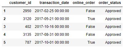
df_final = df[[‘customer_id’,’transaction_date’,’online_order’,’order_status’]]
df_final.head()
df_final = df_final[df_final[‘order_status’] == ‘Approved’]
df_final = df_final[~df_final.duplicated()]
df_final.info()
<class 'pandas.core.frame.DataFrame'>
Int64Index: 19761 entries, 1 to 20000
Data columns (total 4 columns):
 #   Column            Non-Null Count  Dtype
---  ------            --------------  -----
 0   customer_id       19761 non-null  object
 1   transaction_date  19761 non-null  object
 2   online_order      19407 non-null  object
 3   order_status      19761 non-null  object
dtypes: object(4)
memory usage: 771.9+ KB
#Get Transaction Month for the dataframe
import datetime as dt
def get_month(x) :
return dt.datetime(x.year, x.month,1)
df_final[‘transaction_date’] = pd.to_datetime(df[‘transaction_date’])
df_final[‘transaction_month’] = df[‘transaction_date’].apply(get_month)
Step 2: Create Cohort Month and Index
#Create Cohort Month per Rows
group = df_final.groupby(‘customer_id’)[‘transaction_month’]
df_final[‘cohort_month’] = group.transform(‘min’)
#Calculate Cohort Index for Each Rows
def get_date_int(df, column) :
year = df[column].dt.year
month = df[column].dt.month
day = df[column].dt.day
return year, month, day
transaction_year, transaction_month, transaction_day = get_date_int(df_final, ‘transaction_month’)
cohort_year, cohort_month, cohort_day = get_date_int(df_final,’cohort_month’)
#Calculate Year Differences
years_diff = transaction_year – cohort_year
#Calculate Month Differences
months_diff = transaction_month – cohort_month
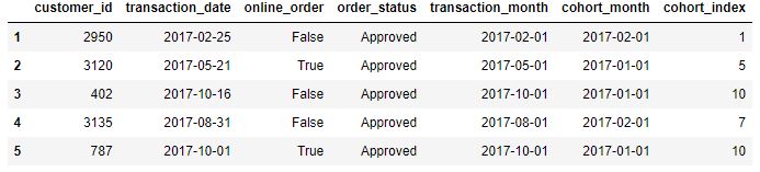
df_final[‘cohort_index’] = years_diff*12 + months_diff + 1
df_final.head()
#Final Grouping to Calculate Total Unique Users in Each Cohort
cohort_group = df_final.groupby([‘cohort_month’,’cohort_index’])
cohort_data = cohort_group[‘customer_id’].apply(pd.Series.nunique)
cohort_data = cohort_data.reset_index()
cohort_counts = cohort_data.pivot_table(index = ‘cohort_month’,
columns = ‘cohort_index’,
values = ‘customer_id’
)
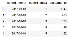
cohort_data.head()
Step 3: Generate User Retention Summary Table
#Calculate Retention rate per Month Index
cohort_size = cohort_counts.iloc[:,0]
retention = cohort_counts.divide(cohort_size, axis = 0)
retention = retention.round(3)*100
retention.index = retention.index.strftime(‘%Y-%m’)
#Plotting Heatmap for Retention Table
import matplotlib.pyplot as plt
import seaborn as sns
plt.figure(figsize = (16,10))
plt.title(‘MoM Retention Rate for Customer Transaction Data’)
sns.heatmap(retention, annot = True, cmap=”YlGnBu”, fmt=’g’)
plt.xlabel(‘Cohort Index’)
plt.ylabel(‘Cohort Month’)
plt.yticks(rotation = ‘360’)
plt.show()

Thus, we have processed transaction data to calculate the customer retention rate per cohort index. Many tech companies use the above heat map to determine whether the campaign is successful or not.


Leave a comment