
Photo by Behnam Norouzi on Unsplash
- The objective of this post is to deploy a Plotly Dash stock market app in Python using the dashboard of user-defined stock prices with popular technical indicators available in TA.
- Read more the tutorial on plotting stock price chart along with volume, MACD & stochastic.
- The entire workflow consists of the following 5 steps:
- Step 1: Select a stock ticker symbol (NVDA) and retrieve stock data frame (df) from yfinance API at an interval of 1m
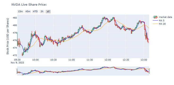
- Step 2: Add Moving Averages (5day and 20day) to df and plot live share price
- Step 3: Add Volume, MACD, and Stochastic Oscillator from TA
- Step 4: Save our stock chart in HTML form, which means all the interactive features will be retained in the graph
- Step 5: Implement the Plotly Dash app containing live NVDA stock prices with MA 5-15-50-200, Volume, RSI, and MACD.
Table of Contents
- Step 1: Imports & Input Data
- Step 2: Add Moving Averages
- Step 3: Add TA Technical Indicators
- Step 4: HTML Chart Output
- Step 5: Implement Plotly Dash App
- Summary
- Explore More
- Appendix: Stock App Functions
Step 1: Imports & Input Data
Let’s set the working directory YOURPATH
import os
os.chdir('YOURPATH')
os. getcwd()
and import/install the following Python libraries
# Raw Package
import numpy as np
import pandas as pd
from pandas_datareader import data as pdr

# Market Data
import yfinance as yf

#Graphing/Visualization
import datetime as dt
import plotly.graph_objs as go

# Override Yahoo Finance
yf.pdr_override()

!pip install ta

from datetime import date
import plotly.graph_objects as go
from plotly.subplots import make_subplots
from ta.trend import MACD
from ta.momentum import RSIIndicator
from dash import html, dcc, Dash
from dash.dependencies import Input, Output, State
# Create input field for our desired stock
stock=input("Enter a stock ticker symbol: ")

# Retrieve stock data frame (df) from yfinance API at an interval of 1m
df = yf.download(tickers=stock,period='1d',interval='1m')

# add Moving Averages (5day and 20day) to df
df['MA5'] = df['Close'].rolling(window=5).mean()
df['MA20'] = df['Close'].rolling(window=20).mean()

print(df)
Enter a stock ticker symbol: NVDA
[*********************100%***********************]  1 of 1 completed
                           Open        High         Low       Close  \
Datetime
2023-11-09 09:30:00  474.670013  478.200012  474.470001  475.755005
2023-11-09 09:31:00  475.880005  476.399597  474.350006  474.899994
2023-11-09 09:32:00  474.935913  475.769989  474.690094  475.160004
2023-11-09 09:33:00  475.179993  476.529999  474.250000  474.950012
2023-11-09 09:34:00  474.940002  476.179993  474.049988  475.079498
...                         ...         ...         ...         ...
2023-11-09 13:04:00  476.597992  477.899994  476.429993  477.899414
2023-11-09 13:05:00  477.899994  478.189911  476.109985  476.390106
2023-11-09 13:06:00  476.512604  476.649994  475.610107  475.709991
2023-11-09 13:07:00  475.660004  476.119995  475.279999  475.474213
2023-11-09 13:08:21  475.261200  475.261200  475.261200  475.261200

                      Adj Close   Volume         MA5        MA20
Datetime
2023-11-09 09:30:00  475.755005  3106825         NaN         NaN
2023-11-09 09:31:00  474.899994   530602         NaN         NaN
2023-11-09 09:32:00  475.160004   278254         NaN         NaN
2023-11-09 09:33:00  474.950012   486628         NaN         NaN
2023-11-09 09:34:00  475.079498   362195  475.168903         NaN
...                         ...      ...         ...         ...
2023-11-09 13:04:00  477.899414   184727  478.246539  479.946407
2023-11-09 13:05:00  476.390106   199381  477.357562  479.808162
2023-11-09 13:06:00  475.709991   213521  476.721240  479.626161
2023-11-09 13:07:00  475.474213   210938  476.382745  479.422871
2023-11-09 13:08:21  475.261200        0  476.146985  479.183136

[215 rows x 8 columns]
Step 2: Add Moving Averages
# Declare plotly figure (go)
fig=go.Figure()

fig.add_trace(go.Candlestick(x=df.index,
                open=df['Open'],
                high=df['High'],
                low=df['Low'],
                close=df['Close'], name = 'market data'))

fig.update_layout(
    title= str(stock)+' Live Share Price:',
    yaxis_title='Stock Price (USD per Shares)')

fig.update_xaxes(
    rangeslider_visible=True,
    rangeselector=dict(
        buttons=list([
            dict(count=15, label="15m", step="minute", stepmode="backward"),
            dict(count=45, label="45m", step="minute", stepmode="backward"),
            dict(count=1, label="HTD", step="hour", stepmode="todate"),
            dict(count=3, label="3h", step="hour", stepmode="backward"),
            dict(step="all")
        ])
    )
)
# Add 5-day Moving Average Trace
fig.add_trace(go.Scatter(x=df.index,
                         y=df['MA5'],
                         opacity=0.7,
                         line=dict(color='blue', width=2),
                         name='MA 5'))
# Add 20-day Moving Average Trace
fig.add_trace(go.Scatter(x=df.index,
                         y=df['MA20'],
                         opacity=0.7,
                         line=dict(color='orange', width=2),
                         name='MA 20'))

fig.show()
Step 3: Add TA Technical Indicators
from ta.trend import MACD
from ta.momentum import StochasticOscillator
# MACD
macd = MACD(close=df['Close'],
            window_slow=26,
            window_fast=12,
            window_sign=9)
# Stochastic
stoch = StochasticOscillator(high=df['High'],
                             close=df['Close'],
                             low=df['Low'],
                             window=14,
                             smooth_window=3)
import plotly
from plotly.subplots import make_subplots

# Declare plotly figure (go)
fig=go.Figure()
# add subplot properties when initializing fig variable ***don't forget to import plotly!!!***
fig = plotly.subplots.make_subplots(rows=4, cols=1, shared_xaxes=True, vertical_spacing=0.01, row_heights=[0.5,0.1,0.2,0.2])
#Full code
import numpy as np
import pandas as pd
from pandas_datareader import data as pdr
from ta.trend import MACD
from ta.momentum import StochasticOscillator

# Market Data
import yfinance as yf

#Graphing/Visualization
import datetime as dt
import plotly
import plotly.graph_objs as go

# Override Yahoo Finance
yf.pdr_override()

# Create input field for our desired stock
stock=input("Enter a stock ticker symbol: ")

# Retrieve stock data frame (df) from yfinance API at an interval of 1m
df = yf.download(tickers=stock,period='1d',interval='1m')

df['MA5'] = df['Close'].rolling(window=5).mean()
df['MA20'] = df['Close'].rolling(window=20).mean()

# MACD
macd = MACD(close=df['Close'],
            window_slow=26,
            window_fast=12,
            window_sign=9)

# stochastic
stoch = StochasticOscillator(high=df['High'],
                             close=df['Close'],
                             low=df['Low'],
                             window=14,
                             smooth_window=3)


# Declare plotly figure (go)
fig=go.Figure()

# add subplot properties when initializing fig variable
fig = plotly.subplots.make_subplots(rows=4, cols=1, shared_xaxes=True,
                    vertical_spacing=0.01,
                    row_heights=[0.5,0.1,0.2,0.2])

fig.add_trace(go.Candlestick(x=df.index,
                open=df['Open'],
                high=df['High'],
                low=df['Low'],
                close=df['Close'], name = 'market data'))

fig.add_trace(go.Scatter(x=df.index,
                         y=df['MA5'],
                         opacity=0.7,
                         line=dict(color='blue', width=2),
                         name='MA 5'))

fig.add_trace(go.Scatter(x=df.index,
                         y=df['MA20'],
                         opacity=0.7,
                         line=dict(color='orange', width=2),
                         name='MA 20'))

# Plot volume trace on 2nd row
colors = ['green' if row['Open'] - row['Close'] >= 0
          else 'red' for index, row in df.iterrows()]
fig.add_trace(go.Bar(x=df.index,
                     y=df['Volume'],
                     marker_color=colors
                    ), row=2, col=1)

# Plot MACD trace on 3rd row
colorsM = ['green' if val >= 0
          else 'red' for val in macd.macd_diff()]
fig.add_trace(go.Bar(x=df.index,
                     y=macd.macd_diff(),
                     marker_color=colorsM
                    ), row=3, col=1)
fig.add_trace(go.Scatter(x=df.index,
                         y=macd.macd(),
                         line=dict(color='black', width=2)
                        ), row=3, col=1)
fig.add_trace(go.Scatter(x=df.index,
                         y=macd.macd_signal(),
                         line=dict(color='blue', width=1)
                        ), row=3, col=1)

# Plot stochastics trace on 4th row
fig.add_trace(go.Scatter(x=df.index,
                         y=stoch.stoch(),
                         line=dict(color='black', width=2)
                        ), row=4, col=1)
fig.add_trace(go.Scatter(x=df.index,
                         y=stoch.stoch_signal(),
                         line=dict(color='blue', width=1)
                        ), row=4, col=1)

# update layout by changing the plot size, hiding legends & rangeslider, and removing gaps between dates
fig.update_layout(height=900, width=1200,
                  showlegend=False,
                  xaxis_rangeslider_visible=False)


# Make the title dynamic to reflect whichever stock we are analyzing
fig.update_layout(
    title= str(stock)+' Live Share Price:',
    yaxis_title='Stock Price (USD per Shares)')

# update y-axis label
fig.update_yaxes(title_text="Price", row=1, col=1)
fig.update_yaxes(title_text="Volume", row=2, col=1)
fig.update_yaxes(title_text="MACD", showgrid=False, row=3, col=1)
fig.update_yaxes(title_text="Stoch", row=4, col=1)

fig.update_xaxes(
    rangeslider_visible=False,
    rangeselector_visible=False,
    rangeselector=dict(
        buttons=list([
            dict(count=15, label="15m", step="minute", stepmode="backward"),
            dict(count=45, label="45m", step="minute", stepmode="backward"),
            dict(count=1, label="HTD", step="hour", stepmode="todate"),
            dict(count=3, label="3h", step="hour", stepmode="backward"),
            dict(step="all")
        ])
    )
)


fig.show()
Enter a stock ticker symbol: NVDA
[*********************100%***********************]  1 of 1 completed
Step 4: HTML Chart Output

fig.write_html(r'filename.html')
Step 5: Implement Plotly Dash App
Let’s invoke the Plotly Dash functions in Appendix and run the app
if __name__ == '__main__':
    application.run(debug = False, port = 8080)
* Running on http://127.0.0.1:8080
Press CTRL+C to quit

Summary
- In this post, we have used Plotly to generate interactive visualizations of NVIDIA stock prices and basic technical indicators from TA
- The Plotly Dash framework has been employed for building web app with the added benefit that no JavaScript is needed.
- Plotly Dash provides increased interactivity and the ability to manipulate data with modern UI elements like dropdowns, sliders and real-time graphs.
- Plotly figures are interactive when viewed in a web browser: we can hover over data points, pan and zoom axes, and show and hide traces by clicking or double-clicking on the legend. We have exported them to HTML files which can be opened in a browser.
- The most significant benefits include our preference for the dashboard layout of all of the charts instead of separate cells of the Jupyter notebook.
- By default, Dash apps run on
localhost. To share a Dash app, we need to deploy it to a server using Dash Enterprise.
Explore More
- Python for Finance: Dash by Plotly
- Deploying Dash Apps
- The $ASML Trading Strategies via the Plotly Stock Market Dashboard
- Datapane Stock Screener App from Scratch
Appendix: Stock App Functions
def makeCandlestick(fig, stockDF):
    #sets parameters for subplots
    fig = make_subplots(rows = 4, cols = 1, shared_xaxes = True,
                    vertical_spacing = 0.01,
                    row_heights = [0.6, 0.1, 0.15, 0.15])


    #plots candlestick values using stockDF
    fig.add_trace(go.Candlestick(x = stockDF.index,
                                 open = stockDF['Open'],
                                 high = stockDF['High'],
                                 low = stockDF['Low'],
                                 close = stockDF['Close'],
                                 name = 'Open/Close'))

    return fig
def makeMA(fig, stockDF):
    #create moving average values
    stockDF["MA5"] = stockDF["Close"].rolling(window = 5).mean()
    stockDF["MA15"] = stockDF["Close"].rolling(window = 15).mean()
    stockDF["MA50"] = stockDF["Close"].rolling(window = 50).mean()
    stockDF["MA200"] = stockDF["Close"].rolling(window = 200).mean()


    #plots moving average values; the 50-day and 200-day averages
    #are visible by default, and the 5-day and 15-day are accessed via legend
    fig.add_trace(go.Scatter(x = stockDF.index, y = stockDF['MA5'], opacity = 0.4, visible="legendonly",
                        line = dict(color = 'blue', width = 2), name = 'MA 5'))

    fig.add_trace(go.Scatter(x = stockDF.index, y = stockDF['MA15'], opacity = 0.7, visible = "legendonly",
                        line = dict(color = 'orangered', width = 2), name = 'MA 15'))

    fig.add_trace(go.Scatter(x = stockDF.index, y = stockDF['MA50'], opacity = 0.7,
                        line = dict(color = 'purple', width = 2), name = 'MA 50'))

    fig.add_trace(go.Scatter(x = stockDF.index, y = stockDF['MA200'], opacity = 0.7,
                        line = dict(color = 'black', width = 2), name = 'MA 200'))

    return fig

def makeVolume(fig, stockDF):
    #sets colors of volume bars
    colors = ['green' if row['Open'] - row['Close'] >= 0
          else 'red' for index, row in stockDF.iterrows()]


    #Plot volume trace
    fig.add_trace(go.Bar(x = stockDF.index,
                         y = stockDF['Volume'],
                         marker_color = colors,
                         showlegend = False,
                         name = "Volume"
                         ), row = 2, col = 1)

    return fig
def makeMACD(fig, stockDF):
    #Create MACD values
    macd = MACD(close = stockDF["Close"],
                window_slow = 26,
                window_fast = 12,
                window_sign = 9)


    #Sets color for MACD
    colors = ['green' if val >= 0
                      else 'red' for val in macd.macd_diff()]


    #Plots MACD values
    fig.add_trace(go.Bar(x = stockDF.index,
                         y = macd.macd_diff(),
                         marker_color = colors,
                         showlegend = False,
                         name = "Histogram"
                         ), row = 4, col = 1)


    fig.add_trace(go.Scatter(x = stockDF.index,
                             y = macd.macd(),
                             line = dict(color = 'red', width = 1),
                             showlegend = False,
                             name = "MACD"
                             ), row = 4, col = 1)


    fig.add_trace(go.Scatter(x = stockDF.index,
                             y = macd.macd_signal(),
                             line = dict(color = 'blue', width = 2),
                             showlegend = False,
                             name = "Signal"
                             ), row = 4, col = 1)


    return fig
def makeRSI(fig, stockDF):
    #Create RSI values
    rsi = RSIIndicator(close = stockDF["Close"],
                       window = 14)


    #Plots RSI values
    fig.add_trace(go.Scatter(x = stockDF.index,
                             y = rsi.rsi(),
                             line = dict(color = 'black', width = 2),
                             showlegend = False,
                             name = "RSI"
                             ), row = 3, col = 1)


    fig.add_trace(go.Scatter(x = stockDF.index,
                             y = [30 for val in range(len(stockDF))],
                             line = dict(color = 'red', width = 1),
                             showlegend = False,
                             name = "Oversold"
                             ), row = 3, col = 1)


    fig.add_trace(go.Scatter(x = stockDF.index,
                             y = [70 for val in range(len(stockDF))],
                             line = dict(color = 'green', width = 1),
                             showlegend = False,
                             name = "Overbought"
                             ), row = 3, col = 1)


    return fig
def makeCurrentPrice(fig, stockDF):
    #Plots the last closing price of stock
    fig.add_trace(go.Scatter(x = stockDF.index,
              y = [stockDF['Close'].iat[-1] for price in range(len(stockDF))],
              opacity = 0.7, line = dict(color = 'red', width = 2, dash = 'dot'),
              name = "Current Price: " + str(round(stockDF['Close'].iat[-1], 2))))


    return fig


def supportLevel(stockDF, index):
    #Finds and returns support levels using fractals;
    #if there are two higher lows on each side of the current stockDF['Low'] value,
    #return this value
    support = stockDF['Low'][index] < stockDF['Low'][index - 1] and \
              stockDF['Low'][index] < stockDF['Low'][index + 1] and \
              stockDF['Low'][index + 1] < stockDF['Low'][index + 2] and \
              stockDF['Low'][index - 1] < stockDF['Low'][index - 2]

    return support


def resistanceLevel(stockDF, index):
    #Finds and returns resistance levels using fractals;
    #If there are two lower highs on each side of the current stock['High'] value,
    #return this value
    resistance = stockDF['High'][index] > stockDF['High'][index - 1] and \
              stockDF['High'][index] > stockDF['High'][index + 1] and \
              stockDF['High'][index + 1] > stockDF['High'][index + 2] and \
              stockDF['High'][index - 1] > stockDF['High'][index - 2]

    return resistance
def isFarFromLevel(stockDF, level, levels):
    #If a level is found near another level, it returns false;

    ##.88 for longer term .97 for short term
    s = np.mean(stockDF['High'] - (stockDF['Low'] * .89))

    return np.sum([abs(level - x) < s for x in levels]) == 0


def makeLevels(fig, stockDF):
    #Traverses through stockDF and finds key support/resistance levels
    levels = []
    for index in range(2, stockDF.shape[0] - 2):
        if supportLevel(stockDF, index):
            support = stockDF['Low'][index]
            if isFarFromLevel(stockDF, support, levels):
                levels.append((support))

        elif resistanceLevel(stockDF, index):
            resistance = stockDF['High'][index]
            if isFarFromLevel(stockDF, resistance, levels):
                levels.append((resistance))

    levels.sort()


    #Plots the key levels within levels
    for i in range(len(levels)):
        fig.add_trace(go.Scatter(x = stockDF.index,
                             y = [levels[i] for val in range(len(stockDF))],
                             line = dict(color = "black"),
                             name = "Sup/Res: " + str(round(levels[i], 2)),
                             hoverinfo = "skip",
                             opacity = 0.3))

    return fig
def findAbsMax(stockDF):
    absMax = 0
    for i in range(len(stockDF)):
        if stockDF["Close"][i] > absMax:
            absMax = stockDF["Close"][i]

    return absMax


def findAbsLow(stockDF):
    absLow = 50
    for i in range(len(stockDF)):
        if stockDF["Close"][i] < absLow:
            absLow = stockDF["Close"][i]

    return absLow


def makeFibLevels(fig, stockDF):
    fibRatios = [.236, .382, .5, .618, .786, 1]
    fibLevels = []
    absMax = findAbsMax(stockDF)
    absLow = findAbsLow(stockDF)
    dif = absMax - absLow

    for i in range(len(fibRatios)):
        fibLevels.append(dif * fibRatios[i])
#for prices that are above the last resistance/support line within fibLevels,
    #look to see if there can be any levels drawn using fractals that are also not
    #too close to the current last support/resistance;
    #We really are just looking for the last resistance level;
    fractal = fibLevels[-1] + (fibLevels[-1] * .17)
    if (fibLevels[-1] < fractal) and (fractal < absMax):
         fibLevels.append(fractal)


    for i in range(len(fibLevels)):
        fig.add_trace(go.Scatter(x = stockDF.index,
                             y = [fibLevels[i] for val in range(len(stockDF))],
                             line = dict(color = "black"),
                             name = "Sup/Res: " + str(round(fibLevels[i], 2)),
                             hoverinfo = "skip",
                             opacity = 0.3))

    return fig


def graphLayout(fig, choice):
    #Sets the layout of the graph and legend
    fig.update_layout(title_text = choice + ' Price Action',
                  title_x = 0.5,
                  legend_title_text = "Legend Items",
                  dragmode = "pan",
                  xaxis_rangeslider_visible = False,
                  hovermode = "x",
                  legend = dict(bgcolor="#E2E2E2",
                           bordercolor="Black",
                           borderwidth=2)

                 )

    subplotLabels(fig)

    return fig
def subplotLabels(fig):
    #Sets subplot labels
    fig.update_yaxes(title_text = "Price", row = 1, col = 1)
    fig.update_yaxes(title_text = "Volume", row = 2, col = 1)
    fig.update_yaxes(title_text = "RSI", row = 3, col = 1)
    fig.update_yaxes(title_text = "MACD", showgrid = False, row = 4, col = 1)

    return fig


def xAxes(fig):
    #Remove none trading days from dataset and sets behavior for x-axis mouse-hovering
    fig.update_xaxes(rangebreaks = [dict(bounds = ["sat", "mon"])],
                 autorange = True,
                 showspikes = True,
                 spikedash = "dot",
                 spikethickness = 1,
                 spikemode = "across",
                 spikecolor = "black")

    return fig


fig = go.Figure()
config = dict({'scrollZoom': True})
stockApp = Dash(__name__, meta_tags=[{'name': 'viewport',
                       'content':'width=device-width, initial-scale=1.0'}])

application = stockApp.server

stockApp.layout = html.Div([
    dcc.Graph(figure = fig, config = config,

              style = {'width': '99vw', 'height': '93vh'},
              id = "stockGraph"
             ),

             html.Div([
                dcc.Input(
                    id = "userInput",
                    type = "text",
                    placeholder = "Ticker Symbol"
                         ),

            html.Button("Submit", id = "btnSubmit")]),
                      ],
            )
 @stockApp.callback(
    Output("stockGraph", "figure"),
    Input("btnSubmit", "n_clicks"),
    State("userInput", "value"))

def update_figure(n, tickerChoice):
    #set choice to something if !isPostBack
    if tickerChoice == None:
        tickerChoice = 'AAPL'


    #make stockDF
    today = date.today()
    stockDF = yf.download(tickerChoice, start = '2020-01-01', end = today )

    #make go Figure object as fig
    fig = go.Figure()

    #make and plot candlestick chart
    fig = makeCandlestick(fig, stockDF)

    #update layout properties
    fig = graphLayout(fig, tickerChoice.upper())

    #updates x-axis parameters
    fig = xAxes(fig)

    #make and plot subplots charts and moving averages
    fig = makeMA(fig, stockDF)
    fig = makeVolume(fig, stockDF)
    fig = makeMACD(fig, stockDF)
    fig = makeRSI(fig, stockDF)

    #make and plot stock's last closing price
    fig = makeCurrentPrice(fig, stockDF)

    #make and plot stock's resistance/support values using fibonacci retracement
    fig = makeFibLevels(fig, stockDF)


    return fig


One-Time
Monthly
Yearly
Make a one-time donation
Make a monthly donation
Make a yearly donation
Choose an amount
€5.00
€15.00
€100.00
€5.00
€15.00
€100.00
€5.00
€15.00
€100.00
Or enter a custom amount
€
Your contribution is appreciated.
Your contribution is appreciated.
Your contribution is appreciated.

Leave a comment