SARIMAX Crude Oil Prices Forecast – 2. Brent

Based on our previous study, our today’s focus is on SARIMAX time-series X-validation of the Brent crude oil spot price USD: viz. the goal is to verify the following EIA energy forecast in 2023

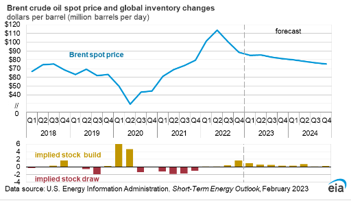
According to EIA, the Brent spot price will average $83.63/b in 2023.

Table of Contents

1. Prerequisites
2. Libraries
3. Input Data
4. ETS Decomposition
5. ADF Test
6. SARIMAX
7. Predictions
8. Residuals
9. Summary
10. Explore More
11. Embed Socials

Prerequisites

In this study we will be installing Anaconda, managing relevant Python-3 packages, creating individual conda environments and sharing them via conda YAML file. One can install multiple packages at the same time. 

Libraries

Let’s set the working directory YOURPATH

import os
os.chdir(‘YOURPATH’)
os. getcwd()

and import/install the following libraries

!pip install statsmodels
!pip install yfinance

import yfinance as yf

import numpy as np
import pandas as pd
from matplotlib import pyplot as plt
from statsmodels.tsa.stattools import adfuller
from statsmodels.tsa.seasonal import seasonal_decompose
from statsmodels.tsa.arima_model import ARIMA
from pandas.plotting import register_matplotlib_converters
register_matplotlib_converters()

from pmdarima import auto_arima

import warnings
warnings.filterwarnings(“ignore”)

!pip install pmdarima

Additional libraries can be imported on the “if-needed” basis.

Input Data

let’s load the input data

df = yf.download(‘BZ=F’, ‘2022-02-03’)

[*********************100%***********************]  1 of 1 completed

Let’s explore the data structure

df.shape

(264, 6)

df.info()

<class 'pandas.core.frame.DataFrame'>
DatetimeIndex: 264 entries, 2022-02-03 to 2023-02-17
Data columns (total 6 columns):
 #   Column     Non-Null Count  Dtype  
---  ------     --------------  -----  
 0   Open       264 non-null    float64
 1   High       264 non-null    float64
 2   Low        264 non-null    float64
 3   Close      264 non-null    float64
 4   Adj Close  264 non-null    float64
 5   Volume     264 non-null    int64  
dtypes: float64(5), int64(1)
memory usage: 14.4 KB

df.describe()

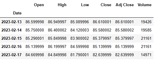
df.tail()

Let’s drop the following columns

df=df.drop([‘Open’, ‘High’, ‘Low’, ‘Close’,’Volume’], axis=1)

to get the single-column table with the time index

df.tail()

Let’s check the null values

df.isnull().sum()

df.isnull().sum()

Adj Close    0
dtype: int64

ETS Decomposition

Let’s perform the seasonal decomposition of our data with model=’multiplicative’ and period=30 (i.e. 1 month)

result = seasonal_decompose(df, model=’multiplicative’,period=30)

result.plot()

ADF Test

Let’s perform the Augmented Dickey-Fuller (ADF) test

adfuller(df[‘Adj Close’])

(-0.8702493547662872,
 0.7976118156481764,
 10,
 253,
 {'1%': -3.4564641849494113,
  '5%': -2.873032730098417,
  '10%': -2.572894516864816},
 1257.2890699767)

Here’s how to interpret the most important values in the output:

• Test statistic: -0.870249
• P-value: 0.79761

Since the p-value is not less than .05, we fail to reject the null hypothesis.

This means the time series is non-stationary in that it has some time-dependent structure and does not have constant variance over time.

SARIMAX

Let’s fit auto_arima function to our input dataset

stepwise_fit = auto_arima(df[‘Adj Close’], start_p = 1, start_q = 1,
max_p = 3, max_q = 3, m = 12,
start_P = 0, seasonal = True,
d = None, D = 1, trace = True,
error_action =’ignore’,
suppress_warnings = True,
stepwise = True)

stepwise_fit.summary()

Performing stepwise search to minimize aic
 ARIMA(1,0,1)(0,1,1)[12] intercept   : AIC=inf, Time=1.00 sec
 ARIMA(0,0,0)(0,1,0)[12] intercept   : AIC=1755.936, Time=0.02 sec
 ARIMA(1,0,0)(1,1,0)[12] intercept   : AIC=1388.994, Time=0.28 sec
 ARIMA(0,0,1)(0,1,1)[12] intercept   : AIC=1574.287, Time=0.28 sec
 ARIMA(0,0,0)(0,1,0)[12]             : AIC=1754.679, Time=0.03 sec
 ARIMA(1,0,0)(0,1,0)[12] intercept   : AIC=1438.019, Time=0.05 sec
 ARIMA(1,0,0)(2,1,0)[12] intercept   : AIC=1357.220, Time=1.05 sec
 ARIMA(1,0,0)(2,1,1)[12] intercept   : AIC=inf, Time=3.20 sec
 ARIMA(1,0,0)(1,1,1)[12] intercept   : AIC=inf, Time=0.87 sec
 ARIMA(0,0,0)(2,1,0)[12] intercept   : AIC=1738.787, Time=0.72 sec
 ARIMA(2,0,0)(2,1,0)[12] intercept   : AIC=1358.635, Time=1.18 sec
 ARIMA(1,0,1)(2,1,0)[12] intercept   : AIC=1358.655, Time=1.28 sec
 ARIMA(0,0,1)(2,1,0)[12] intercept   : AIC=1570.019, Time=0.87 sec
 ARIMA(2,0,1)(2,1,0)[12] intercept   : AIC=1360.622, Time=2.68 sec
 ARIMA(1,0,0)(2,1,0)[12]             : AIC=1355.364, Time=0.30 sec
 ARIMA(1,0,0)(1,1,0)[12]             : AIC=1387.045, Time=0.09 sec
 ARIMA(1,0,0)(2,1,1)[12]             : AIC=inf, Time=1.39 sec
 ARIMA(1,0,0)(1,1,1)[12]             : AIC=inf, Time=0.78 sec
 ARIMA(0,0,0)(2,1,0)[12]             : AIC=1740.760, Time=0.18 sec
 ARIMA(2,0,0)(2,1,0)[12]             : AIC=1356.815, Time=0.38 sec
 ARIMA(1,0,1)(2,1,0)[12]             : AIC=1356.832, Time=0.36 sec
 ARIMA(0,0,1)(2,1,0)[12]             : AIC=1572.157, Time=0.30 sec
 ARIMA(2,0,1)(2,1,0)[12]             : AIC=1358.807, Time=0.81 sec

Best model:  ARIMA(1,0,0)(2,1,0)[12]          
Total fit time: 18.091 seconds

SARIMAX Results:

Dep. Variable:	y	No. Observations:	264
Model:	SARIMAX(1, 0, 0)x(2, 1, 0, 12)	Log Likelihood	-673.682
Date:	Fri, 17 Feb 2023	AIC	1355.364
Time:	10:36:45	BIC	1369.482
Sample:	0	HQIC	1361.045
	– 264
Covariance Type:	opg

	coef	std err	z	P>|z|	[0.025	0.975]
ar.L1	0.9165	0.019	47.894	0.000	0.879	0.954
ar.S.L12	-0.6100	0.049	-12.357	0.000	-0.707	-0.513
ar.S.L24	-0.4017	0.052	-7.708	0.000	-0.504	-0.300
sigma2	11.9008	0.874	13.617	0.000	10.188	13.614

Ljung-Box (L1) (Q):	0.61	Jarque-Bera (JB):	14.30
Prob(Q):	0.44	Prob(JB):	0.00
Heteroskedasticity (H):	0.24	Skew:	-0.01
Prob(H) (two-sided):	0.00	Kurtosis:	4.17

let’s split the data into train / test sets
train = df.iloc[:len(df)-12]
test = df.iloc[len(df)-12:] # set one year(12 months) for testing

and fit the SARIMAX(1, 0, 0)x(2, 1, 0, 12) model to the training set

from statsmodels.tsa.statespace.sarimax import SARIMAX
model = SARIMAX(train[‘Adj Close’],
order = (0, 1, 0),
seasonal_order =(2, 1, 0, 12))
result = model.fit()
result.summary()

SARIMAX Results:

Dep. Variable:	Adj Close	No. Observations:	252
Model:	SARIMAX(0, 1, 0)x(2, 1, 0, 12)	Log Likelihood	-647.761
Date:	Fri, 17 Feb 2023	AIC	1301.521
Time:	10:37:05	BIC	1311.951
Sample:	0	HQIC	1305.724
	– 252
Covariance Type:	opg

	coef	std err	z	P>|z|	[0.025	0.975]
ar.S.L12	-0.6397	0.047	-13.476	0.000	-0.733	-0.547
ar.S.L24	-0.4151	0.048	-8.736	0.000	-0.508	-0.322
sigma2	12.8359	0.969	13.246	0.000	10.937	14.735

Ljung-Box (L1) (Q):	0.01	Jarque-Bera (JB):	19.35
Prob(Q):	0.92	Prob(JB):	0.00
Heteroskedasticity (H):	0.25	Skew:	-0.40
Prob(H) (two-sided):	0.00	Kurtosis:	4.14

• Goodness of fit test, The Jarque-Bera test is a goodness-of-fit test that measures if sample data has skewness and kurtosis that are similar to a normal distribution. The JB test statistic is always positive, and if it is not close to zero, it shows that the sample data do not have a normal distribution.
• Negative skew refers to a longer or fatter tail on the left side of the distribution.
• Positive excess values of kurtosis (>3) indicate that a distribution is peaked and possess thick tails. Leptokurtic distributions have positive kurtosis values.
• A leptokurtic distribution has a higher peak (thin bell) and taller (i.e. fatter and heavy) tails than a normal distribution.

Predictions

Let’s print our test data and 1Y predictions

print(test[‘Adj Close’],predictions)

Date
2023-02-02    82.169998
2023-02-03    79.940002
2023-02-06    80.989998
2023-02-07    83.690002
2023-02-08    85.089996
2023-02-09    84.500000
2023-02-10    86.389999
2023-02-13    86.610001
2023-02-14    85.580002
2023-02-15    85.379997
2023-02-16    85.139999
2023-02-17    83.680000
Name: Adj Close, dtype: float64 252    84.005361
253    85.602957
254    86.011120
255    84.965660
256    84.457512
257    84.003784
258    84.321574
259    85.826474
260    85.605278
261    86.496948
262    86.800109
263    85.527856
Name: Predictions, dtype: float64

Let’s plot test data vs predictions

x=test[‘Adj Close’]
y=predictions
plt.plot(x,y, ‘o’, color=’green’)

get m (slope) and b(intercept) of a linear regression line
m, b = np.polyfit(x, y, 1)

use red as a color for the linear regression line
plt.plot(x, m*x+b, color=’red’)
plt.xlabel(‘Adj Close Test’)
plt.ylabel(‘Predictions’)

Train the model on the full dataset
model = model = SARIMAX(df[‘Adj Close’],
order = (0, 1, 1),
seasonal_order =(2, 1, 1, 12))
result = model.fit()

Forecast for 1Y
forecast = result.predict(start = len(df),
end = (len(df)-1) + 1 * 12,
typ = ‘levels’).rename(‘Forecast’)

Plot the forecast values vs train data
df[‘Adj Close’].plot(figsize = (2, 5), legend = True)
forecast.plot(legend = True)

Let’s plot the forecast

print(forecast)

264    82.930292
265    82.569673
266    82.759312
267    81.629149
268    82.420565
269    82.121951
270    82.551539
271    82.931898
272    82.737850
273    82.810189
274    83.249728
275    83.419509
Name: Forecast, dtype: float64

a = np.array([‘Jan’, ‘Feb’, ‘Mar’,’Apr’,’May’,’Jun’,’Jul’,’Aug’,’Sept’,’Oct’,’Nov’,’Dec’])
plt.plot(a,forecast)
plt.xlabel(“Month 2023”);
plt.ylabel(“Predicted Brent Oil Price $”);

Overall, this plot supports the EIA energy forecast in 2023 within the confidence intervals defined below.

Residuals

Let’s evaluate our predictions by using the following sklearn error metrics

from sklearn.metrics import mean_squared_error
from statsmodels.tools.eval_measures import rmse

rmse(test[“Adj Close”], predictions)

2.5038953839620026

mean_squared_error(test[“Adj Close”], predictions)

6.2694920938262255

Summary

• The ADF test show that our time series dataset is non-stationary. In other words, it has some time-dependent structure and does not have constant variance over time.
• The seasonal decomposition of our dataset reveals the distinct trend curve and the prominent seasonal effect.
• Our train/test dataset does not have a normal distribution – negative skew refers to a longer or fatter tail on the left side of the distribution; positive excess value of kurtosis (>3) indicates that our distribution is peaked and possess thick tails (Leptokurtic distribution).
• Our predictions ca. $83.4 (Dec 2023) are generally consistent with the EIA energy forecast in 2023 (ca. $83.63/b).
• Remaining discrepancies are well within the predicted confidence intervals +/- $6.

Explore More

SARIMAX X-Validation of EIA Crude Oil Prices Forecast in 2023 – 1. WTI

OXY Stock Analysis, Thursday, 23 June 2022

Energy E&P: XOM Technical Analysis Nov ’22

Embed Socials

#commodity #energy #Oil #Oilprices #forecast (s)#arima(x) vs @IEA #WTI #brentpetrol #CrudeOil @tradingview #ChartStories @SeekingAlpha #ideas #validation #comparison#results support @JPMorganAM #strategy #downgrade #Oilprices#DataScience #Algorithms https://t.co/kRjVrIjfym

— Alex Z. data4u #va #DataScience #investments (@AlexZaplin) February 5, 2023

---