
- YouTube (YT) is probably the most popular web platform that is easy to share non-textual content such as videos and animations.
- The goal of this post is to get data science insights into YouTube trending videos for many countries, to see what is common between these videos.
- Specifically, the following questions need to be answered: How many views, likes and comments do our trending videos have? How are views, likes, dislikes, comment count, title length, and other attributes correlate with each other? What are the most common words in trending video titles? Which video category has the largest number of trending videos?
- Method: Python NLP statistics and sentiment analysis in a variety of forms, including Exploratory Data Analysis (EDA) & Vis.
Table of Contents
- Global YT WordCloud
- US YT Videos
- Global YT Videos
- IN YT Trending Video Dataset
- US/CA YT trending Analysis
- US YT EDA 2020-2023
- US YT NLP Sentiment Analysis
- US YT NLP Category Prediction
- Summary
- Explore More
- Embed Socials
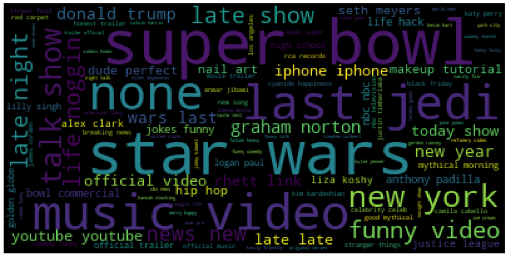
Global YT WordCloud
Let’s begin with the Kaggle YT TextHero dataset containing 3599 rows and 4 columns.
Let’s set the working directory YOURPATH
import os
os.chdir(‘YOURPATH’)
os. getcwd()
and import all necessary modules
from wordcloud import WordCloud, STOPWORDS
import matplotlib.pyplot as plt
import pandas as pd
Let’s read the input dataset
df = pd.read_csv(r”youtube0.csv”, encoding =”latin-1″)
df.head()

and set STOPWORDS
comment_words = ”
stopwords = set(STOPWORDS)
Let’s iterate through the csv file
for val in df.title:
val = str(val)
# split the value
tokens = val.split()

# Converts each token into lowercase
for i in range(len(tokens)):
    tokens[i] = tokens[i].lower()

comment_words += " ".join(tokens)+" "
wordcloud = WordCloud(width = 800, height = 800,
background_color =’white’,
stopwords = stopwords,
min_font_size = 10).generate(comment_words)
and plot the WordCloud image
plt.figure(figsize = (8, 8), facecolor = None)
plt.imshow(wordcloud)
plt.axis(“off”)
plt.tight_layout(pad = 0)
plt.savefig(‘youtubewordcloudsongs.png’)

US YT Videos
Let’s look at the Kaggle US videos dataset containing 40949 rows and 16 columns:
- video_id
- trending_date
- title
- channel_title
- category_id
- publish_time
- tags
- views
- likes
- dislikes
- comment_count
- thumbnail_link
- comments_disabled
- ratings_disabled
- video_error_or_removed
- description
Let’s import the key libraries
import numpy as np
import pandas as pd
import seaborn as sns
import matplotlib.pyplot as plt
from wordcloud import WordCloud, STOPWORDS, ImageColorGenerator
and read the input dataset
df = pd.read_csv(“USvideos.csv”)
df.tail()


df.shape
(40949, 16)
Let’s check isnull
df.isnull().sum()
video_id                    0
trending_date               0
title                       0
channel_title               0
category_id                 0
publish_time                0
tags                        0
views                       0
likes                       0
dislikes                    0
comment_count               0
thumbnail_link              0
comments_disabled           0
ratings_disabled            0
video_error_or_removed      0
description               570
dtype: int64
and compute the correlation matrix
df.corr(method=’pearson’)

The corresponding sns heatmap is
import seaborn as sns
import matplotlib.pyplot as plt
sns.heatmap(df.corr())

Let’s translate the category names
df[‘category_name’] = np.nan
df.loc[(df[“category_id”] == 1),”category_name”] = ‘Film and Animation’
df.loc[(df[“category_id”] == 2),”category_name”] = ‘Cars and Vehicles’
df.loc[(df[“category_id”] == 10),”category_name”] = ‘Music’
df.loc[(df[“category_id”] == 15),”category_name”] = ‘Pets and Animals’
df.loc[(df[“category_id”] == 17),”category_name”] = ‘Sport’
df.loc[(df[“category_id”] == 19),”category_name”] = ‘Travel and Events’
df.loc[(df[“category_id”] == 20),”category_name”] = ‘Gaming’
df.loc[(df[“category_id”] == 22),”category_name”] = ‘People and Blogs’
df.loc[(df[“category_id”] == 23),”category_name”] = ‘Comedy’
df.loc[(df[“category_id”] == 24),”category_name”] = ‘Entertainment’
df.loc[(df[“category_id”] == 25),”category_name”] = ‘News and Politics’
df.loc[(df[“category_id”] == 26),”category_name”] = ‘How to and Style’
df.loc[(df[“category_id”] == 27),”category_name”] = ‘Education’
df.loc[(df[“category_id”] == 28),”category_name”] = ‘Science and Technology’
df.loc[(df[“category_id”] == 29),”category_name”] = ‘Non Profits and Activism’
df.loc[(df[“category_id”] == 25),”category_name”] = ‘News & Politics’
and count their values as
print(df.category_name.value_counts())
Entertainment               9964
Music                       6472
How to and Style            4146
Comedy                      3457
People and Blogs            3210
News & Politics             2487
Science and Technology      2401
Film and Animation          2345
Sport                       2174
Education                   1656
Pets and Animals             920
Gaming                       817
Travel and Events            402
Cars and Vehicles            384
Non Profits and Activism      57
Name: category_name, dtype: int64
Let’s plot these counts
plt.figure(figsize = (16,9))
ax = sns.countplot(x=”category_name”, data=df, orient =’H’)
for bar in ax.patches:
if bar.get_height() > 8000:
bar.set_color(‘red’)
else:
bar.set_color(‘grey’)
ax.set_xticklabels(ax.get_xticklabels(), rotation=45)
ax.set_title(“Counting the Video Category’s “, fontsize=15)
ax.set_xlabel(”, fontsize=12)
ax.set_ylabel(“Count”, fontsize=12)
plt.savefig(‘usvideocategories.png’)

Let’s check the YT publish time variable
best_count = df[[‘channel_title’, ‘views’, ‘publish_time’]]
best_count = best_count.sort_values(‘views’, ascending = False)
best_count[‘publish_time’] = pd.DatetimeIndex(df[‘publish_time’]).year

Similarly, we can check likes/year
like= df[[‘likes’, ‘publish_time’]]
plt.figure(figsize = (16,9))
like[‘publish_time’] = pd.DatetimeIndex(like[‘publish_time’]).year
ax = sns.countplot(x=”publish_time”, data=like)
ax.set_title(“Likes per Year”, fontsize=15)
ax.set_xlabel(”, fontsize=12)
ax.set_ylabel(“Likes”, fontsize=12)
plt.savefig(‘uslikesperyear.png’)

Let’s plot the WordCloud
plt.subplots(figsize=(25,15))
wordcloud = WordCloud(
background_color=’black’,
width=1920,
height=1080
).generate(” “.join(df.channel_title))
plt.imshow(wordcloud)
plt.axis(‘off’)
plt.savefig(‘usvideocategory.png’)

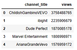
Let’s count US views per YT channel
Best_twl = df[[‘channel_title’, ‘views’]]
Best_twl = Best_twl.groupby(‘channel_title’)[‘views’].sum()
Best_twl = pd.DataFrame(Best_twl)
Best_twl = Best_twl.sort_values(‘views’, ascending=False)
Best_twl = Best_twl[:12]
Best_twl= Best_twl.reset_index()
Best_twl.head()
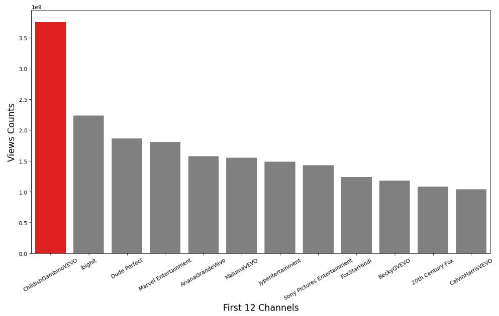
Let’s plot these views as a bar plot
plt.figure(figsize=(15, 8))
c = [‘red’, ‘grey’, ‘grey’, ‘grey’, ‘grey’, ‘grey’, ‘grey’, ‘grey’, ‘grey’, ‘grey’, ‘grey’, ‘grey’]
ax = sns.barplot(data = Best_twl, x = ‘channel_title’, y =’views’, palette =c)
ax.set_xticklabels(labels= Best_twl.channel_title, fontsize=10, rotation=30)
ax.set_xlabel(xlabel=’First 12 Channels’, fontsize=16)
ax.set_ylabel(ylabel=’Views Counts’, fontsize=16)
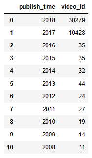
Let’s look at video_id vs publish time
year = df[[‘publish_time’,’video_id’]]
year[‘publish_time’] = pd.DatetimeIndex(year[‘publish_time’]).year
year = year.groupby(‘publish_time’)[‘video_id’].count()
year = pd.DataFrame(year)
year = year.sort_values(‘publish_time’, ascending=False)
year= year.reset_index()
year.head(11)
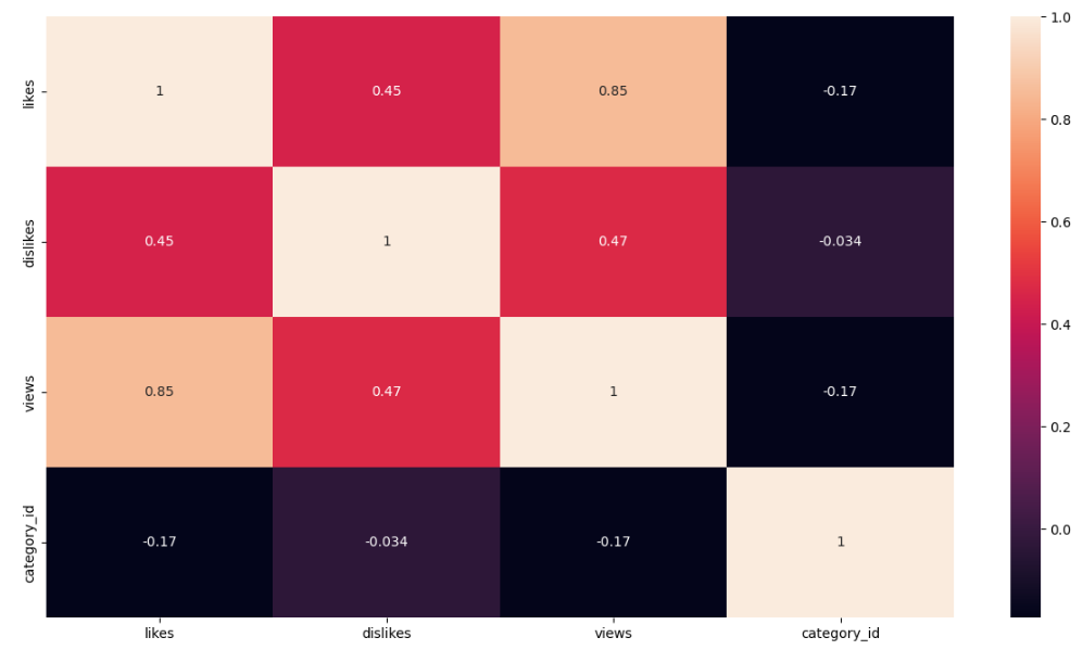
Let’s looks at the sns correlation heatmap of the following attributes
df_1 = df[[‘likes’, ‘dislikes’, ‘views’, ‘category_id’]]
plt.figure(figsize=(15, 8))
sns.heatmap(df_1.corr(),annot=True)
Global YT Videos
Let’s import the libraries
import numpy as np
import pandas as pd
import csv
import datetime
import math
import json
import datetime
from IPython.core.display import HTML
import matplotlib
import plotly
import plotly.graph_objects as go
import plotly.express as px
from plotly.subplots import make_subplots
import warnings
warnings.filterwarnings(“ignore”)
and load the input dataset representing trending global YT videos
countries = [“CA”, “DE”, “FR”, “GB”, “IN”, “KR”, “MX”, “RU”, “US”]
country_names = [“Canada”, “Germany”, “France”, “Great Britain”, “India”, “South Korea”, “Mexico”, “Russia”, “United States”]
df_youtube = pd.DataFrame()
for i in range(len(countries)):
if(countries[i] in [“KR”, “MX”, “RU”]):
df_country = pd.read_csv(“{}videos.csv”.format(countries[i]), encoding=”latin-1″)
else:
df_country = pd.read_csv(“{}videos.csv”.format(countries[i]))
df_country[“country”] = country_names[i]
df_youtube = pd.concat([df_youtube, df_country], ignore_index=True, sort=False)
Let’ drop duplicates and check the shape
print(“Before Drop Duplicates:”, df_youtube.shape)
df_youtube = df_youtube.drop_duplicates()
print(” After Drop Duplicates:”, df_youtube.shape)
df_youtube = df_youtube[df_youtube[“category_id”]!=29]
category_id = {}
with open(‘CA_category_id.json’, ‘r’) as f:
data = json.load(f)
for category in data[‘items’]:
category_id[int(category[‘id’])] = category[‘snippet’][‘title’]
df_youtube = df_youtube.replace({“category_id”: category_id})
Before Drop Duplicates: (355419, 17)
After Drop Duplicates: (348526, 17)
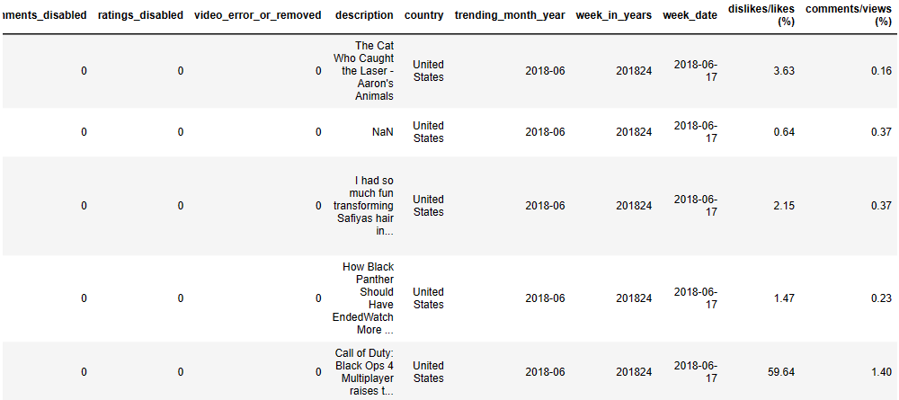
Let’s perform the following data editing steps:
- Change Date Features from Object to Date
df_youtube[‘trending_date’] = pd.to_datetime(df_youtube[‘trending_date’], format=’%y.%d.%m’)
df_youtube[‘trending_month_year’] = pd.to_datetime(df_youtube[‘trending_date’]).dt.to_period(‘M’)
df_youtube[“publish_time”] = pd.to_datetime(df_youtube[‘publish_time’], format=’%Y-%m-%dT%H:%M:%S.%fZ’)
df_youtube[“week_in_years”] = df_youtube[“trending_date”].dt.strftime(‘%Y%W’)
df_youtube[“week_date”] = pd.to_datetime(df_youtube[“week_in_years”]+’0′, format=’%Y%W%w’)
df_youtube[“week_date”] = df_youtube[“week_date”].dt.strftime(‘%Y-%m-%d’)
- Create Ratio from Viewer Behavioral Features
df_youtube[“dislikes/likes (%)”] = round((df_youtube[“dislikes”] / df_youtube[“likes”]) * 100, 2)
df_youtube[“comments/views (%)”] = round((df_youtube[“comment_count”] / df_youtube[“views”]) * 100, 2)
- Change Channel Behavioral Features from Boolean to Binary Values
df_youtube[“comments_disabled”] = df_youtube[“comments_disabled”].replace([False, True], [0, 1])
df_youtube[“ratings_disabled”] = df_youtube[“ratings_disabled”].replace([False, True], [0, 1])
df_youtube[“video_error_or_removed”] = df_youtube[“video_error_or_removed”].replace([False, True], [0, 1])
Let’s check the updated data structure
print(df_youtube.shape)
df_youtube.tail()
(345772, 22)

Let’s prepare our plots:
- DataFrame
category_count = df_youtube.groupby([“category_id”])[“video_id”].count().reset_index()
category_count = category_count.rename(columns={“video_id”: “total”}).sort_values(by=”total”, ascending=False).reset_index(drop=True)
total = category_count[“total”].sum()
category_count[“percentages”] = round((category_count[“total”]/total)*100, 1)
category_count = category_count[:10].sort_index(ascending=False).reset_index(drop=True)
- Create Figure
fig = go.Figure() - Define colour map
cmap = matplotlib.colors.LinearSegmentedColormap.from_list(“”, [“#6fd404″,”#649e3c”, “#0c2304”])
min_color = category_count[“percentages”].min()
max_color = category_count[“percentages”].max()
colors = []
for i in range(10):
color = cmap(i/9)
color = matplotlib.colors.rgb2hex(color)
colors.append(color)
Let’s construct the Lollipop Chart “Top 10 Most Trending Videos by Categories”
from matplotlib import pyplot as plt
fig.add_trace(
go.Scatter(
x=category_count[“percentages”],
y=category_count[“category_id”],
mode=’markers+text’,
marker=dict(
color=colors,
size=50,
),
text=[“{}%”.format(x) for x in category_count[“percentages”]],
textposition=”middle center”,
textfont=dict(
size=15,
color=”White”
),
)
)
for i in range(10):
fig.add_shape(type=”line”,
x0=0.0, y0=i, x1=category_count[“percentages”][i]-1.38, y1=i,
line=dict(
color=colors[i],
width=6
)
)
fig.update_xaxes(title_text=””, showticklabels=False, showgrid=False, range=[0,35])
fig.update_yaxes(title_text=””, showticklabels=True, showgrid=False)
fig.update_layout(title_text=’Top 10 Most Trending Videos by Categories’,
title_x=0.5,
font=dict(
family=”Times New Roman”,
size=15,
),
margin=dict(
pad=20
),
width=900, height=820,
plot_bgcolor=’White’,
showlegend=False,
)
fig.show()

Let’s create the plot “The Number of Trending Videos by Categories”:
category_count_time = pd.DataFrame(df_youtube.groupby([“category_id”, “week_date”])[“video_id”].count().unstack(fill_value=0).stack())
category_count_time = category_count_time.rename(columns={0: “total”})
category_count_time = category_count_time.reset_index()
fig = go.Figure()
list_category = category_count_time[“category_id”].unique().tolist()
array_week_date = list(range(len(category_count_time[“week_date”].unique())))
week_date = category_count_time[“week_date”].unique().tolist()
highlight_categories = [“Entertainment”, “People & Blogs”, “Film & Animation”]
annotations = list(fig[‘layout’][‘annotations’])
for i in range(len(list_category)):
youtube_category = category_count_time[category_count_time[“category_id”]==list_category[i]]
opacity = 0.25
if(list_category[i] in highlight_categories):
opacity = 1.0
fig.add_trace(
go.Scatter(
x=array_week_date,
y=youtube_category[“total”],
mode=”lines”,
line=dict(
color=”#649e3c”, width=2
),
name=list_category[i],
text=week_date,
opacity=opacity,
hovertemplate=
‘Week Date: %{text}
‘+
‘Total : %{y}’,
)
)
# Annotations
if(list_category[i] in highlight_categories):
annotations.append(
dict(
xref=”paper”, yref=”y1″, xanchor=”left”,
x=0.94, y=youtube_category.iloc[-1, -1],
text=list_category[i],
font=dict(
family=”Times New Roman”,
size=13,
color=”#649e3c”
),
showarrow=False
)
)
fig[‘layout’].update(annotations=annotations)
fig.update_xaxes(title_text=””,
showticklabels=True, showgrid=False, linecolor=”Gray”, ticks=’outside’, range=[0, array_week_date[-1]+2],
tickmode=’array’, tickvals=[0, 6, 12, 18, 24, 30], ticktext=category_count_time[“week_date”].unique()[[0, 6, 12, 18, 24, 30]]
)
fig.update_yaxes(title_text=””,
showticklabels=True, showgrid=False, linecolor=”Gray”, ticks=’outside’,
)
fig.update_layout(title_text=”The Number of Trending Videos by Categories”,
title_x=0.5,
font=dict(
family=”Times New Roman”,
size=13.5,
),
width=800,
height=600,
plot_bgcolor=’White’,
showlegend=False,
)
fig.show()

Similarly, we can compare Likes of Trending Videos by Country as a boxplot
fig = go.Figure()
country_likes = df_youtube[[“country”, “week_date”, “likes”]]
country_likes = country_likes.groupby([“country”, “week_date”])[“likes”].mean().reset_index()
top_country_likes = country_likes.groupby([“country”])[“likes”].mean().reset_index()
top_country_likes = top_country_likes.sort_values(by=”likes”, ascending=True).reset_index(drop=True)
cmap = matplotlib.colors.LinearSegmentedColormap.from_list(“”, [“#6fd404″,”#649e3c”, “#0c2304”])
colors = []
for i in range(len(top_country_likes)):
country = top_country_likes[“country”][i]
youtube_country = country_likes[country_likes[“country”]==country]
color = cmap(i/(len(top_country_likes)-1))
color = matplotlib.colors.rgb2hex(color)

fig.add_trace(
    go.Box(
        x=youtube_country["likes"],
        marker_color=color,
        name=country
    )
)
fig.update_xaxes(title_text=””,
showticklabels=True,
showgrid=True, gridcolor=’#eeeeee’)
fig.update_yaxes(title_text=””,
showticklabels=True,
showgrid=True, gridcolor=’#eeeeee’)
fig.update_layout(title_text=”Likes of Trending Videos by Country”,
title_x=0.5,
font=dict(
family=”Times New Roman”,
size=13.5,
),
width=900,
height=600,
plot_bgcolor=’White’,
showlegend=False,
)
fig.show()

Let’s prepare our data for trellis_chart:
- Update Category
category_id = [“Sports”, “Film & Animation”, “Howto & Style”, “Gaming”]
df_youtube = df_youtube[df_youtube[“category_id”].isin(category_id)]
df_youtube[“category_id”] = df_youtube[“category_id”].replace([“Film & Animation”, “Howto & Style”], [“Film and Animation”, “How to and Styles”])
- Video Count
video_count = df_youtube[[“week_date”, “category_id”, “country”]]
video_count = pd.DataFrame(video_count.groupby([“category_id”, “week_date”, “country”])[“country”].count().unstack(fill_value=0).stack())
video_count = video_count.rename(columns={0: “total”})
video_count = video_count.reset_index()
- Video Count Trend in One Day
video_count_one_day = df_youtube[[“trending_date”, “publish_time”, “week_date”, “category_id”, “country”]]
video_count_one_day[“trend_publish_one_day”] = video_count_one_day[“trending_date”]-video_count_one_day[“publish_time”]
video_count_one_day[“days”] = (video_count_one_day[“trend_publish_one_day”].astype(‘timedelta64[D]’) + 1).astype(int)
video_count_one_day = video_count_one_day[video_count_one_day[“days”]<=1]
video_count_one_day = video_count_one_day.drop(“trend_publish_one_day”, axis=1)
video_count_one_day = pd.DataFrame(video_count_one_day.groupby([“category_id”, “week_date”, “country”])[“country”].count().unstack(fill_value=0).stack())
video_count_one_day = video_count_one_day.rename(columns={0: “total”})
video_count_one_day = video_count_one_day.reset_index()
- Dislikes/Likes Ratio Percentages
dislikes_likes_ratio = df_youtube[[“week_date”, “likes”, “category_id”, “dislikes/likes (%)”, “country”]]
dislikes_likes_ratio = dislikes_likes_ratio[dislikes_likes_ratio[“likes”]!=0]
dislikes_likes_ratio = pd.DataFrame(dislikes_likes_ratio.groupby([“category_id”, “week_date”, “country”])[“dislikes/likes (%)”].mean().unstack(fill_value=-1).stack()).reset_index()
dislikes_likes_ratio = dislikes_likes_ratio.rename(columns={0: “dislikes/likes (%)”})
dislikes_likes_ratio[“dislikes/likes (%)”] = dislikes_likes_ratio[“dislikes/likes (%)”].replace(to_replace=-1,value=dislikes_likes_ratio[“dislikes/likes (%)”].mean())
- Comments/Views Ratio Percentages
comments_views_ratio = df_youtube[[“week_date”, “category_id”, “comments/views (%)”, “country”]]
comments_views_ratio = pd.DataFrame(comments_views_ratio.groupby([“category_id”, “week_date”, “country”])[“comments/views (%)”].mean().unstack(fill_value=-1).stack()).reset_index()
comments_views_ratio = comments_views_ratio.rename(columns={0: “comments/views (%)”})
comments_views_ratio[“comments/views (%)”] = comments_views_ratio[“comments/views (%)”].replace(to_replace=-1,value=comments_views_ratio[“comments/views (%)”].mean())
- Content Creator Behavioral
channel_behavioral = df_youtube[[“week_date”, “category_id”, “country”, “comments_disabled”, “ratings_disabled”, “video_error_or_removed”]]
channel_behavioral[“total_disabled”] = channel_behavioral[“comments_disabled”] + channel_behavioral[“ratings_disabled”] + channel_behavioral[“video_error_or_removed”]
channel_behavioral = pd.DataFrame(channel_behavioral.groupby([“category_id”, “week_date”, “country”])[“total_disabled”].mean().unstack(fill_value=-1).stack()).reset_index()
channel_behavioral = channel_behavioral.rename(columns={0: “mean_disabled”})
channel_behavioral[“mean_disabled”] = channel_behavioral[“mean_disabled”].replace(to_replace=-1,value=channel_behavioral[“mean_disabled”].mean())
Let’s define the corresponding plotting functions:
def draw_trellis_chart(df, category, column, title):
# Create Subplots
fig = make_subplots(rows=3, cols=3, vertical_spacing=0.005, horizontal_spacing=0.005)
# Trellis Chart
youtube = df[df["category_id"]==category]
max_range = youtube[column].max()
top_2_country = youtube.sort_values(by=column, ascending=False)["country"].unique().tolist()[:2]
top_2_color = ["#93c0be", "#bfeae8"]
array_week_date = list(range(len(df["week_date"].unique())))
week_date = youtube["week_date"].unique().tolist()

for i in range(len(country_names)):
    youtube_country = youtube[youtube["country"]==country_names[i]]
    fig.add_trace(
        go.Scatter(
            x=array_week_date,
            y=youtube_country[column],
            mode="lines",
            line=dict(
                color="#737e7e", width=2
            ),
           line_shape="spline",
            name=country_names[i],
            text=week_date,
            hovertemplate=
            'Week Date: %{text}<br>'+
            'Measures : %{y}',
        ), row=i//3+1, col=i%3+1
    )

    # Highest Point
    max_total = youtube_country[column].max()
    x_point = youtube_country[youtube_country[column]==max_total]["week_date"].values[0]
    x_point = week_date.index(x_point)
    max_total = round(max_total, 2)
    fig.add_trace(
        go.Scatter(
            x=[x_point], y=[max_total],
            mode='markers',
            marker=dict(
                color="#737e7e",
                size=6.5,
            ),
            hovertemplate=
            '<b>Highest Point</b><br>'+
            'Week Date: %{x}<br>'+
            'Measures : %{y}',
            name=country_names[i]
       ), row=i//3+1, col=i%3+1
    )

    # Text
    annotations = list(fig['layout']['annotations'])
    bold = ""
    if(country_names[i] in top_2_country):
        bold = "<b>"
    annotations.append(dict(xref='x{}'.format(i+1), yref='y{}'.format(i+1), xanchor="center", x=15, y=max_range*1.5,
                            text="{}{}".format(bold, country_names[i]),
                            font=dict(
                                family="Times New Roman",
                                size=14,
                            ),
                            showarrow=False)
    )
    annotations.append(dict(xref='x{}'.format(i+1), yref='y{}'.format(i+1), xanchor="center", x=15, y=max_range*1.32,
                            text="Highest Point: {}".format(max_total),
                            font=dict(
                                family="Times New Roman",
                                size=10,
                            ),
                            showarrow=False)
    )
    fig['layout'].update(annotations=annotations)
    # Background Color
    shapes = list(fig['layout']['shapes'])
    if(country_names[i]==top_2_country[0]):
        bg_color = top_2_color[0]
    elif(country_names[i]==top_2_country[1]):
        bg_color = top_2_color[1]
    else:
        bg_color = "#ebebeb"

    shape = dict(
        type="rect",
        xref="x{}".format(i+1), yref="y{}".format(i+1),
        x0=-2, x1=array_week_date[-1]+2,
        y0=0-max_range*0.3, y1=max_range*1.6,
        fillcolor=bg_color,
        opacity=0.7,
        layer="below",
        line_width=0,
    )
    shapes.append(shape)

    fig.update_layout(shapes=shapes,)

    # Update Axes
    fig.update_xaxes(title_text="",
                     showline=False, showticklabels=False, showgrid=False, zeroline=False,
                     row=i//3+1, col=i%3+1,
                     range=[-2, array_week_date[-1]+2])
    fig.update_yaxes(title_text="",
                     showline=False, showticklabels=False, showgrid=False, zeroline=False,
                     row=i//3+1, col=i%3+1,
                     range=[0-max_range*0.3, max_range*1.6])

# Update Layout
fig.update_layout(title_text="{} in Each Country".format(title),
                  title_x=0.5,
                  font=dict(
                    family="Times New Roman",
                    size=15,
                  ),
                  width=700,
                  height=700,
                  plot_bgcolor='#ebebeb',
                  showlegend=False,
)

# Show
fig.show()

return top_2_country[0]
def draw_highlight_line_chart(df, category, column, country, title):
# Create Figure
fig = go.Figure()
youtube_country = df[(df[“category_id”]==category)&(df[“country”]==country)]
array_week_date = list(range(len(df[“week_date”].unique())))
week_date = youtube_country[“week_date”].unique().tolist()
# Line Chart
fig.add_trace(
    go.Scatter(
        x=array_week_date,
        y=youtube_country[column],
        mode="lines",
        line_shape="spline",
        line=dict(
            color="#18b53f", width=3
        ),
        text=week_date,
        hovertemplate=
            'Week Date: %{text}<br>'+
            'Measures : %{y}',
        name=country
    )
)

# Update Axes

fig.update_xaxes(title_text="",
                 showticklabels=True, showgrid=False, linecolor="Gray", ticks='outside', range=[0, array_week_date[-1]+1],
                 tickmode='array', tickvals=[0, 6, 12, 18, 24, 30], ticktext=youtube_country["week_date"].unique()[[0, 6, 12, 18, 24, 30]]
                )
fig.update_yaxes(title_text="",
                 showticklabels=True, showgrid=False, linecolor="Gray", ticks='outside',
                )

# Update Layout
    fig.update_layout(title_text="{} in {}".format(title, country),
                      title_x=0.5,
                      font=dict(
                        family="Times New Roman",
                        size=13.5,
                      ),
                      width=700,
                      height=350,
                      plot_bgcolor='White',
                      showlegend=False,
    )

    # Show
    fig.show()
Category Sports
Let’s choose the Category
category = “Sports”
and plot the Video Count per Country
title = “The Number of Trending {} Videos”.format(category)
country = draw_trellis_chart(video_count, category, “total”, title)
draw_highlight_line_chart(video_count, category, “total”, country, title)
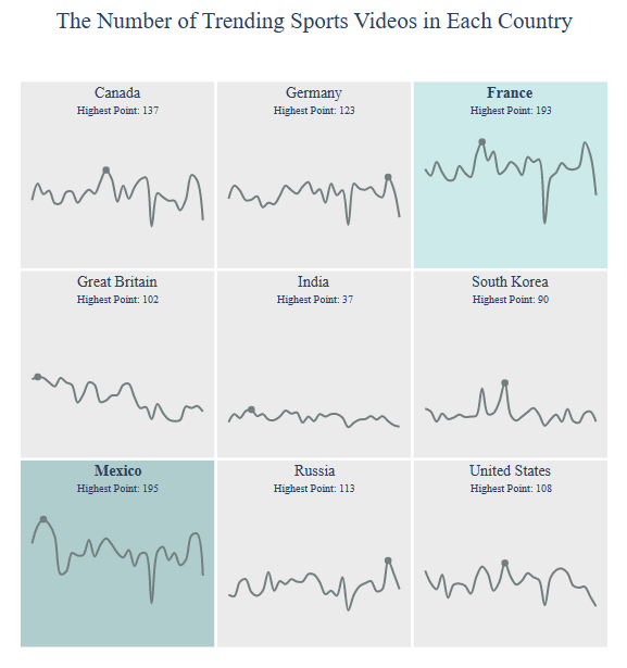
For example, the number of trending sport videos in Mexico is

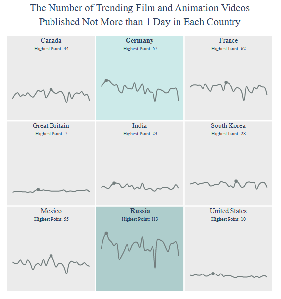
Let’s look at the Number of Trending Global YT Videos Published Not More than 1 Day per Country
title = “The Number of Trending {} Videos
Published Not More than 1 Day”.format(category)
country = draw_trellis_chart(video_count_one_day, category, “total”, title)
draw_highlight_line_chart(video_count_one_day, category, “total”, country, title)
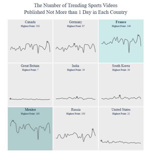
For example, the number of trending sports YT videos published not more than 1 day in Mexico is given by

Dislikes/Likes Ratio Percentages:
title = “Dislikes/Likes Ratio Percentages on
{} Videos”.format(category)
country = draw_trellis_chart(dislikes_likes_ratio, category, “dislikes/likes (%)”, title)
draw_highlight_line_chart(dislikes_likes_ratio, category, “dislikes/likes (%)”, country, title)

For example, Dislikes/Likes Ratio Percentages on sports YT videos in Mexico is

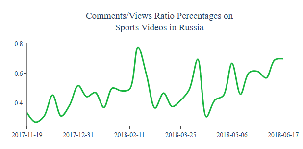
Comments/Views Ratio Percentages:
title = “Comments/Views Ratio Percentages on
{} Videos”.format(category)
country = draw_trellis_chart(comments_views_ratio, category, “comments/views (%)”, title)
draw_highlight_line_chart(comments_views_ratio, category, “comments/views (%)”, country, title)
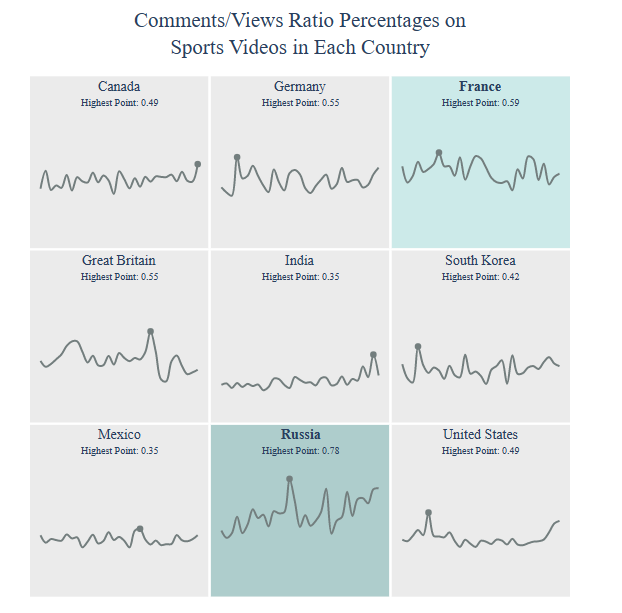
For example, Comments/Views Ratio Percentages in Russia are
Channel Behavioral:
title = “Channel Behavioral Measures on
{} Videos”.format(category)
country = draw_trellis_chart(channel_behavioral, category, “mean_disabled”, title)
draw_highlight_line_chart(channel_behavioral, category, “mean_disabled”, country, title)
Let’s select the Category
category = “Film and Animation”
and compute the Video Count per country
title = “The Number of Trending {} Videos”.format(category)
country = draw_trellis_chart(video_count, category, “total”, title)
draw_highlight_line_chart(video_count, category, “total”, country, title)

For example, Channel Behavioral Measures on Sports Videos in South Korea are

Category Film and Animation
Let’s select the Category
category = “Film and Animation”
and count the number of trending film and animation videos per country
title = “The Number of Trending {} Videos”.format(category)
country = draw_trellis_chart(video_count, category, “total”, title)
draw_highlight_line_chart(video_count, category, “total”, country, title)

For example, the number of trending film and animation videos in Great Britain is

Let’s check Video Count (Published Not More than 1 Day)
title = “The Number of Trending {} Videos
Published Not More than 1 Day”.format(category)
country = draw_trellis_chart(video_count_one_day, category, “total”, title)
draw_highlight_line_chart(video_count_one_day, category, “total”, country, title)
including those in Russia

Let’s check the Dislikes/Likes Ratio Percentages per Country
title = “Dislikes/Likes Ratio Percentages on
{} Videos”.format(category)
country = draw_trellis_chart(dislikes_likes_ratio, category, “dislikes/likes (%)”, title)
draw_highlight_line_chart(dislikes_likes_ratio, category, “dislikes/likes (%)”, country, title)

including those in Great Britain

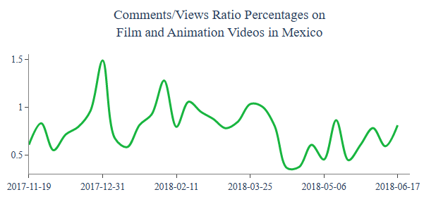
Let’s look at Comments/Views Ratio Percentages
title = “Comments/Views Ratio Percentages on
{} Videos”.format(category)
country = draw_trellis_chart(comments_views_ratio, category, “comments/views (%)”, title)
draw_highlight_line_chart(comments_views_ratio, category, “comments/views (%)”, country, title)

including those in Mexico
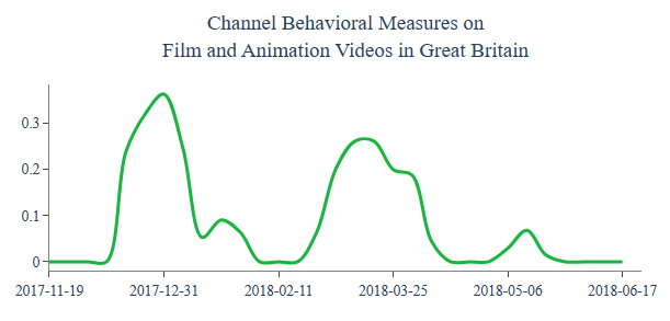
Let’s check Channel Behavioral for “Film and Animation” videos per country
title = “Channel Behavioral Measures on
{} Videos”.format(category)
country = draw_trellis_chart(channel_behavioral, category, “mean_disabled”, title)
draw_highlight_line_chart(channel_behavioral, category, “mean_disabled”, country, title)

including those in Great Britain
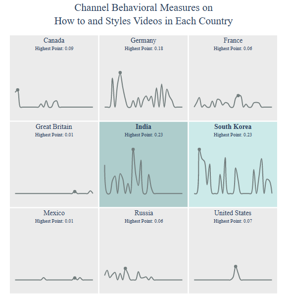
Category How to and Styles
Let’s select Category
category = “How to and Styles”
and get Video Count for this category per country
title = “The Number of Trending {} Videos”.format(category)
country = draw_trellis_chart(video_count, category, “total”, title)
draw_highlight_line_chart(video_count, category, “total”, country, title)

including those in USA

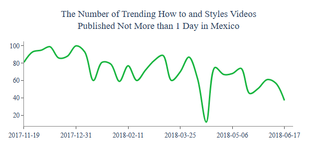
Let’s get Video Count (Published Not More than 1 Day) per country
title = “The Number of Trending {} Videos
Published Not More than 1 Day”.format(category)
country = draw_trellis_chart(video_count_one_day, category, “total”, title)
draw_highlight_line_chart(video_count_one_day, category, “total”, country, title)
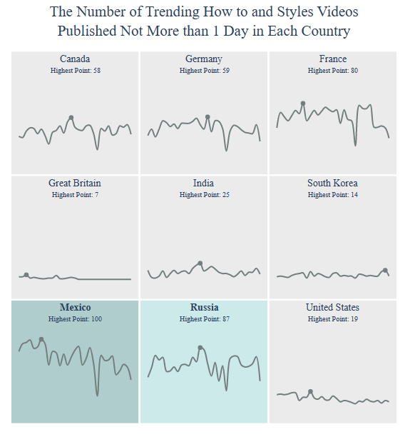
including those in Mexico
Dislikes/Likes Ratio Percentages per country:
title = “Dislikes/Likes Ratio Percentages on
{} Videos”.format(category)
country = draw_trellis_chart(dislikes_likes_ratio, category, “dislikes/likes (%)”, title)
draw_highlight_line_chart(dislikes_likes_ratio, category, “dislikes/likes (%)”, country, title)
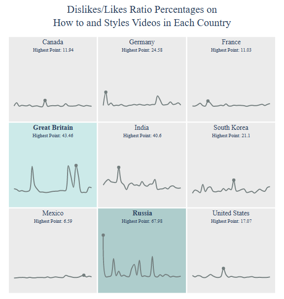
Dislikes/Likes Ratio Percentages in Russia:

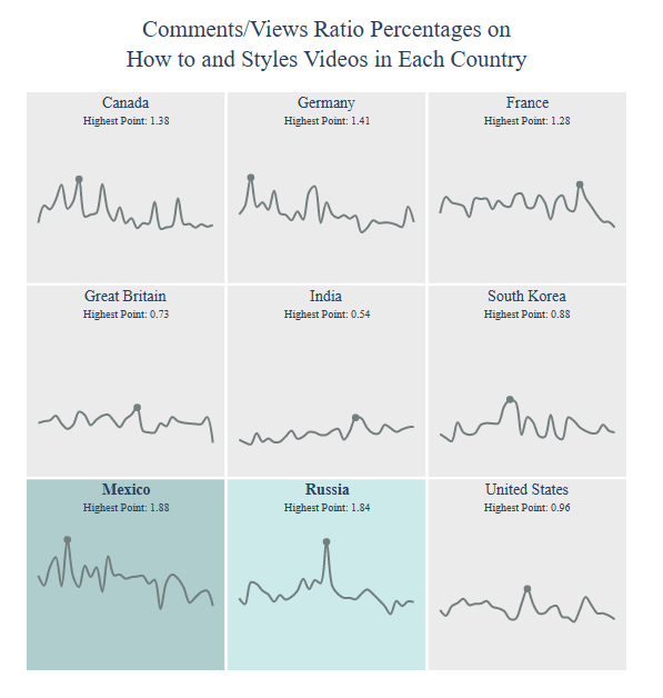
Comments/Views Ratio Percentages:
title = “Comments/Views Ratio Percentages on
{} Videos”.format(category)
country = draw_trellis_chart(comments_views_ratio, category, “comments/views (%)”, title)
draw_highlight_line_chart(comments_views_ratio, category, “comments/views (%)”, country, title)

Channel Behavioral:
title = “Channel Behavioral Measures on
{} Videos”.format(category)
country = draw_trellis_chart(channel_behavioral, category, “mean_disabled”, title)
draw_highlight_line_chart(channel_behavioral, category, “mean_disabled”, country, title)

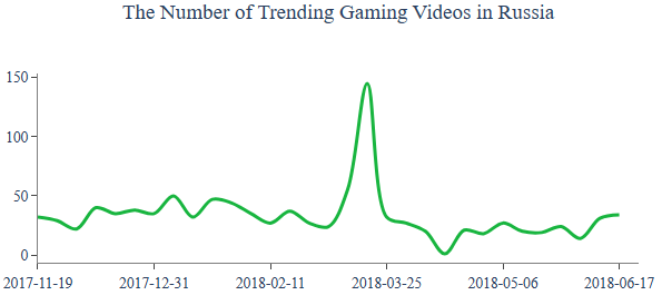
Category Gaming
Let’s select Category
category = “Gaming”
Video Count:
title = “The Number of Trending {} Videos”.format(category)
country = draw_trellis_chart(video_count, category, “total”, title)
draw_highlight_line_chart(video_count, category, “total”, country, title)

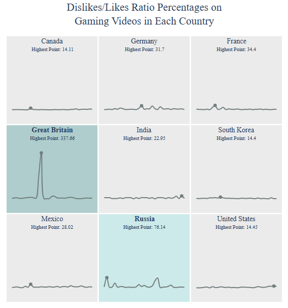
Dislikes/Likes Ratio Percentages:
title = “Dislikes/Likes Ratio Percentages on
{} Videos”.format(category)
country = draw_trellis_chart(dislikes_likes_ratio, category, “dislikes/likes (%)”, title)
draw_highlight_line_chart(dislikes_likes_ratio, category, “dislikes/likes (%)”, country, title)

Comments/Views Ratio Percentages:
title = “Comments/Views Ratio Percentages on
{} Videos”.format(category)
country = draw_trellis_chart(comments_views_ratio, category, “comments/views (%)”, title)
draw_highlight_line_chart(comments_views_ratio, category, “comments/views (%)”, country, title)


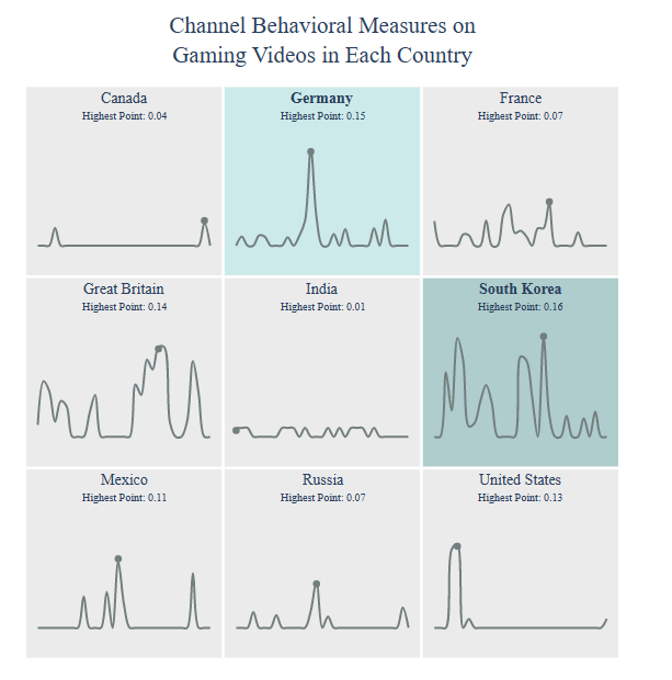
Channel Behavioral:
title = “Channel Behavioral Measures on
{} Videos”.format(category)
country = draw_trellis_chart(channel_behavioral, category, “mean_disabled”, title)
draw_highlight_line_chart(channel_behavioral, category, “mean_disabled”, country, title)

IN YT Trending Video Dataset
Let’s consider the Kaggle YT trending video dataset 2020-2023 (updated daily) and select country=IN.
Let’s import the key libraries and read both json metadata and the actual csv dataset
import pandas as pd
import numpy as np
import seaborn as sns
import matplotlib.pyplot as plt
import warnings
from scipy import stats
from sklearn import preprocessing
from sklearn.preprocessing import scale
import plotly.express as px
warnings.filterwarnings(‘ignore’)
sns.set(style=”whitegrid”)
df_json = pd.read_json(“IN_category_id.json”)
Creating dictionary for json file provided for category and category id
category_dict = {}
for i in df_json[‘items’]:
category_dict[i[‘id’]] = i[‘snippet’][‘title’]
Reading the actual data
df = pd.read_csv(“IN_youtube_trending_data.csv”)
df.tail(3)
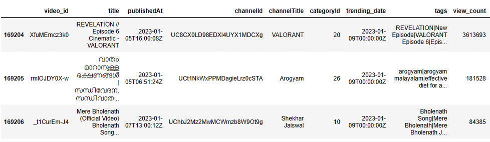

df.shape
(169207, 16)
df.info()
<class 'pandas.core.frame.DataFrame'>
RangeIndex: 169207 entries, 0 to 169206
Data columns (total 16 columns):
 #   Column             Non-Null Count   Dtype
---  ------             --------------   -----
 0   video_id           169207 non-null  object
 1   title              169207 non-null  object
 2   publishedAt        169207 non-null  object
 3   channelId          169207 non-null  object
 4   channelTitle       169206 non-null  object
 5   categoryId         169207 non-null  int64
 6   trending_date      169207 non-null  object
 7   tags               169207 non-null  object
 8   view_count         169207 non-null  int64
 9   likes              169207 non-null  int64
 10  dislikes           169207 non-null  int64
 11  comment_count      169207 non-null  int64
 12  thumbnail_link     169207 non-null  object
 13  comments_disabled  169207 non-null  bool
 14  ratings_disabled   169207 non-null  bool
 15  description        152140 non-null  object
dtypes: bool(2), int64(5), object(9)
memory usage: 18.4+ MB
Dropping some columns not intending to use
df = df.drop([‘video_id’,’thumbnail_link’,’channelId’],axis=1)
Replacing the category id with category actual name by writing a simple function and passing with df.apply
def replace_categoryid(df):
if str(df) in category_dict:
return category_dict[str(df)]
df[‘category’] = df[‘categoryId’].apply(replace_categoryid)
and apply drop to categoryId
df = df.drop([‘categoryId’],axis=1)
df.info()
<class 'pandas.core.frame.DataFrame'>
RangeIndex: 169207 entries, 0 to 169206
Data columns (total 13 columns):
 #   Column             Non-Null Count   Dtype
---  ------             --------------   -----
 0   title              169207 non-null  object
 1   publishedAt        169207 non-null  object
 2   channelTitle       169206 non-null  object
 3   trending_date      169207 non-null  object
 4   tags               169207 non-null  object
 5   view_count         169207 non-null  int64
 6   likes              169207 non-null  int64
 7   dislikes           169207 non-null  int64
 8   comment_count      169207 non-null  int64
 9   comments_disabled  169207 non-null  bool
 10  ratings_disabled   169207 non-null  bool
 11  description        152140 non-null  object
 12  category           169134 non-null  object
dtypes: bool(2), int64(4), object(7)
memory usage: 14.5+ MB
Converting two date time columns to appropriate datetime formats
df[‘publishedAt’] = pd.to_datetime(df[‘publishedAt’])
df[‘trending_date’] = pd.to_datetime(df[‘trending_date’])
Checking for null or missing values present in the data
df.isnull().sum()
title                    0
publishedAt              0
channelTitle             1
trending_date            0
tags                     0
view_count               0
likes                    0
dislikes                 0
comment_count            0
comments_disabled        0
ratings_disabled         0
description          17067
category                73
dtype: int64
Let’s apply fillna to the following 3 columns
df[‘category’] = df[‘category’].fillna(“Other”)
df[‘channelTitle’] = df[‘channelTitle’].fillna(“Juvis Productions”)
df[‘description’] = df[‘description’].fillna(‘No description provided’)
Let’s drop duplicates while keeping the last recorded video in the list
df = df.drop_duplicates(‘title’,keep=’last’)
channel_group_df = df.groupby(by = df[‘channelTitle’]).sum()
channel_group_df[channel_group_df[‘view_count’] == channel_group_df[‘view_count’].max()]
channelTitle: T-Series
| view_count 3992568922 | likes 107288675 | dislikes 3915517 | comment_count 7231286 | comments_disabled 0 | ratings_disabled 1 |
|---|
Plotting the top 5 channels with max view count, likes, dislikes, and comment_count
plt.figure(figsize = (18,8))
plt.subplot(2,2,1)
var_list = [‘view_count’,’likes’,’dislikes’,’comment_count’]
for i in range(0,4):
plt.subplot(2,2,i+1)
x = channel_group_df[var_list[i]].nlargest(5).index
y = channel_group_df[var_list[i]].nlargest(5)
sns.barplot(x = x,y = y)
plt.savefig(‘indiatop5chanmaxviewcount.png’)

Let’s group our input data by category
category_group_df = df.groupby(by = df[‘category’]).sum()
category_group_df

Let’s check max view_count with category=Entertainment
category_group_df[category_group_df[‘view_count’] == category_group_df[‘view_count’].max()]

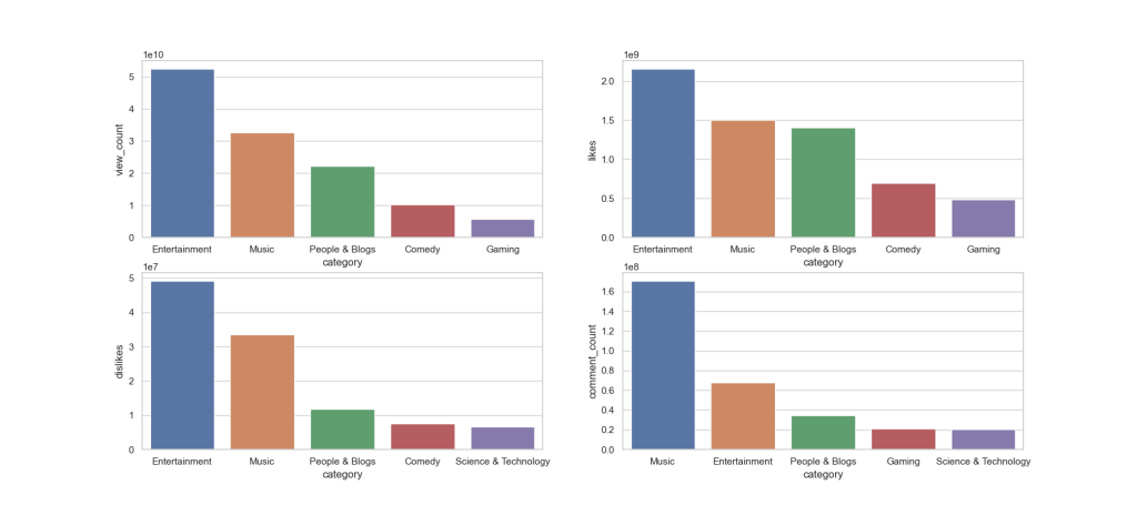
Plotting the top 5 categories with max view count, likes, dislikes, and comment_count
plt.figure(figsize = (18,8))
plt.subplot(2,2,1)
var_list = [‘view_count’,’likes’,’dislikes’,’comment_count’]
for i in range(0,4):
plt.subplot(2,2,i+1)
x = category_group_df[var_list[i]].nlargest(5).index
y = category_group_df[var_list[i]].nlargest(5)
sns.barplot(x = x,y = y)
plt.savefig(‘indiatop5chanmaxviewcountentertainment.png’)
Plotting the top 5 Categories with min view count, likes, dislikes, and comment_count
plt.figure(figsize = (20,8))
plt.subplot(2,2,1)
var_list = [‘view_count’,’likes’,’dislikes’,’comment_count’]
for i in range(0,4):
plt.subplot(2,2,i+1)
x = category_group_df[var_list[i]].nsmallest(5).index
y = category_group_df[var_list[i]].nsmallest(5)
sns.barplot(x = x,y = y)
plt.savefig(‘indiatop5chanminviewcountentertainment.png’)

Let’s count comments_disabled per category
disabled_comments_df =df[df[‘comments_disabled’] == True]
disabled_comments_df[‘category’].value_counts()
Entertainment           163
People & Blogs           95
News & Politics          76
Science & Technology     48
Comedy                   24
Music                    14
Film & Animation          7
Education                 5
Howto & Style             5
Gaming                    4
Sports                    3
Travel & Events           2
Autos & Vehicles          1
Name: category, dtype: int64
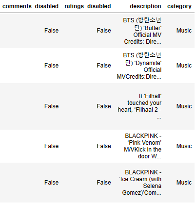
Let’s look at most viewed top 5 videos in 2020 data
df_2020 = df[df[‘publishedAt’].dt.year == 2020]
df_2020[df_2020[‘view_count’].isin(df_2020[‘view_count’].nlargest(5))].sort_values(‘view_count’,ascending = False)
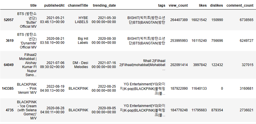
Let’s check 2021 videos
df_2021 = df[df[‘publishedAt’].dt.year == 2021]
df_2021[df_2021[‘view_count’].isin(df_2021[‘view_count’].nlargest(5))].sort_values(‘view_count’,ascending = False)
Let’s check 2022 videos
df_2022 = df[df[‘publishedAt’].dt.year == 2022]
df_2022[df_2022[‘view_count’].isin(df_2022[‘view_count’].nlargest(5))].sort_values(‘view_count’,ascending = False)
Let’s create the column of unique category by appending view_count.max()
cat_list = list(df[‘category’].unique())
cat_data = pd.DataFrame()
for i in cat_list:
cat_data = cat_data.append(df[df[‘view_count’] == (df[df[‘category’] == i].view_count.max())])
cat_data
| Title | publishedAt | channelTitle | trending_date | tags | view_count | likes | dislikes | comment_count | comments_disabled | ratings_disabled | description | category |
|---|
| Dr. Dre, Snoop Dogg, Eminem, Mary J. Blige & K… | 2022-02-14 01:37:03+00:00 | NFL | 2022-02-18 00:00:00+00:00 | Cincinnati Bengals|Los Angeles Rams | 52504127 | 1906350 | 0 | 135887 | False | False | Check out our other channels:NFL Mundo https:/… | Sports | |
| 93154 | OMG Hot burger! 😂 #shorts Best video by MoniLina | 2021-12-06 05:00:32+00:00 | MoniLina | 2021-12-14 00:00:00+00:00 | [None] | 84994444 | 0 | 0 | 2010 | False | True | Thank you for watching our channel MoniLina!Pl… | Comedy |
|---|---|---|---|---|---|---|---|---|---|---|---|---|---|
| 113075 | jai shree ram 🚩#shorts #ashortaday | 2022-03-15 03:21:02+00:00 | CHANDAN ART ACADEMY | 2022-03-25 00:00:00+00:00 | [None] | 155975017 | 8196855 | 0 | 49866 | False | False | No description provided | Education |
| 57398 | Paytm IPL 2021 Ad – The Salon (English) | 2021-06-08 14:24:24+00:00 | Paytm | 2021-06-14 00:00:00+00:00 | [None] | 141191928 | 2297 | 2257 | 711 | False | False | No description provided | People & Blogs |
| 52057 | BTS (방탄소년단) ‘Butter’ Official MV | 2021-05-21 03:46:13+00:00 | HYBE LABELS | 2021-05-30 00:00:00+00:00 | BIGHIT|빅히트|방탄소년단|BTS|BANGTAN|방탄 | 264407389 | 16021542 | 150990 | 6738565 | False | False | BTS (방탄소년단) ‘Butter’ Official MV Credits: Dire… | Music |
| 86718 | 😬Bike vs Man challange😍😍😍#ytshortsindia #usa_s… | 2021-11-01 02:00:54+00:00 | MR.INDIAN HACKER {#Shorts} | 2021-11-10 00:00:00+00:00 | [None] | 48123437 | 2554591 | 53513 | 2532 | False | False | Short#viral#tranding_video #viral#a2motivation… | Autos & Vehicles |
| 13357 | Apple Event — October 13 | 2020-10-13 18:15:12+00:00 | Apple | 2020-10-20 00:00:00+00:00 | Apple|Event|Keynote|Tim Cook|October|2020|Laun… | 53596388 | 922165 | 53076 | 0 | True | False | Watch the special Apple Event and learn about … | Science & Technology |
| 104602 | Betiyaan kisi se kam nahi hoti || Gulshan kalr… | 2022-02-01 07:49:36+00:00 | Gulshan Kalra | 2022-02-10 00:00:00+00:00 | [None] | 65891951 | 4002304 | 0 | 2986 | False | False | No description provided | Howto & Style |
| 115052 | Watch the uncensored moment Will Smith smacks … | 2022-03-28 03:06:53+00:00 | Guardian News | 2022-04-04 00:00:00+00:00 | Jada Pinkett Smith|Jada Pinkett Smith chris ro… | 91180111 | 1335555 | 0 | 236855 | False | False | Best actor nominee Will Smith appeared to slap… | News & Politics |
| 51797 | Money Plinko Challenge! 💰 #shorts | 2021-05-14 22:57:41+00:00 | AnthonySenpai | 2021-05-23 00:00:00+00:00 | [None] | 72699576 | 1934690 | 70207 | 4650 | False | False | No description provided | Gaming |
| 141971 | “Bhai ka farz har kadam pe🙏” #littleglove #ash… | 2022-08-10 07:00:30+00:00 | LittleGlove | 2022-08-18 00:00:00+00:00 | [None] | 40533294 | 2871153 | 0 | 3727 | False | False | No description provided | Travel & Events |
| 115254 | KGF Chapter 2 Trailer|Hindi|Yash|Sanjay Dutt|R… | 2022-03-27 13:10:32+00:00 | Excel Movies | 2022-04-05 00:00:00+00:00 | KGF Chapter 2|KGF Chapter 2 Trailer|Yash|Rocki… | 78319334 | 3298598 | 0 | 153989 | False | False | KGF Chapter 2 releases on 14th April, 2022Pres… | Film & Animation |
| 65239 | Yes or No Challenge 😂 #shorts | 2021-07-15 06:42:08+00:00 | Jenni’s Hacks | 2021-07-22 00:00:00+00:00 | [None] | 5292130 | 145882 | 8011 | 734 | False | False | Yes or No Challenge 😂 #shorts #jennishacks Don… | Other |
| 134419 | Oddly satisfying 🤪🤪🤪 Kids don’t try at home #t… | 2022-07-04 01:49:54+00:00 | That Little Puff | 2022-07-11 00:00:00+00:00 | [None] | 92597901 | 4564339 | 0 | 3976 | False | False | No description provided | Pets & Animals |
In [32]:
df['publishedAt'].dt.year.value_counts().plot
Let’s plot overall year.value_counts() for 2020-2023
df[‘publishedAt’].dt.year.value_counts().plot(kind = ‘bar’)

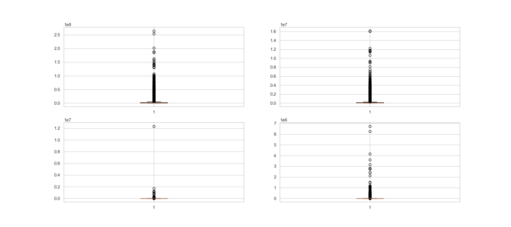
Let’s plot boxplots of India ‘view_count’, ‘likes’, ‘dislikes’, and ‘comment_count’
plt.figure(figsize = (18,8))
plt.subplot(2,2,1)
distributions = [‘view_count’, ‘likes’, ‘dislikes’, ‘comment_count’]
for i in range(0,4):
plt.subplot(2,2,i+1)
plt.boxplot(df[distributions[i]])
plt.savefig(‘indiaboxplotsviewcountslikescomments.png’)
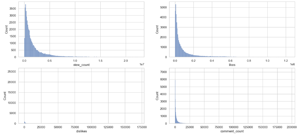
Let’s plot histograms of India ‘view_count’, ‘likes’, ‘dislikes’, and ‘comment_count’
plt.figure(figsize = (18,8))
plt.subplot(2,2,1)
distributions = [‘view_count’, ‘likes’, ‘dislikes’, ‘comment_count’]
for i in range(0,4):
plt.subplot(2,2,i+1)
z = np.abs(stats.zscore(df[distributions[i]]))
outliers = df.iloc[np.where(z > 3)]
outliers_removed_df = df[~df.isin(outliers)].dropna(how=’all’)
sns.histplot(x = distributions[i],data = outliers_removed_df)
plt.savefig(‘indiahistviewcountslikescomments.png’)
Let’s compare mean and median of India Likes
df[‘likes’].mean()
138655.47157818155
df[‘likes’].median()
40833.0
Let’s plot the correlation heatmap
plt.figure(figsize=(16,6))
sns.heatmap(df.corr(),annot=True)
plt.savefig(‘indiaheatmapcorrmap.png’)
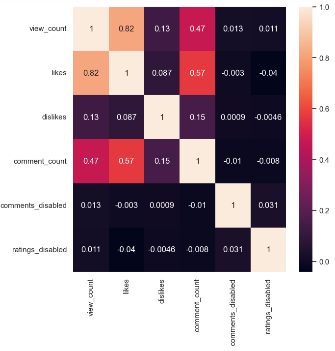
Plotting view_count vs likes as the above heatmap shows a high correlation between these two variables
plt.figure(figsize=(12,5))
sns.lmplot(x = ‘view_count’,y = ‘likes’, data = df)
plt.savefig(‘indiaxplotlikesviews.png’)

Let’s plot India View Count with Time Slider
fig = px.line(df, x=’trending_date’, y = ‘view_count’, title = “View Count with Slider”)
fig.update_xaxes(rangeslider_visible = True)
fig.show()
Full range 2020-2023
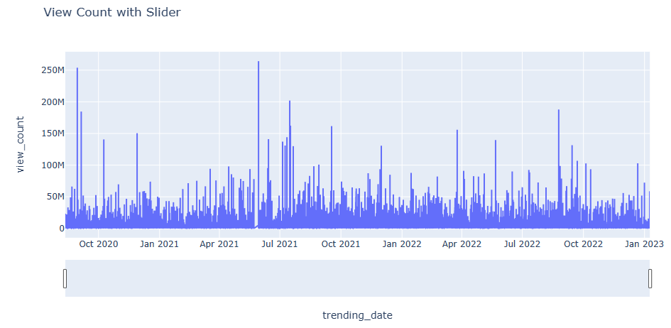
Second half of 2022 and January 2023

US/CA YT trending Analysis
Following earlier studies, let’s examine the Mitchell J’s Trending YouTube Videos Statistics dataset representing the US and CA videos.
Let’s import the libraries and load the input data
import pandas as pd
import matplotlib.pyplot as plt
import numpy as np
data_canada = pd.read_csv(‘CAvideos.csv’, encoding=’utf8′)
data_us = pd.read_csv(‘USvideos.csv’, encoding=’utf8′)
data_us.tail()


Let’s extract the following 9 columns from input dataframes
dc_r = data_canada.iloc[:, [0, 1, 2, 3, 4, 7, 8, 9, 10]].copy()
dus_r = data_us.iloc[:, [0, 1, 2, 3, 4, 7, 8, 9, 10]].copy()
dus_r.info()
<class 'pandas.core.frame.DataFrame'>
RangeIndex: 40949 entries, 0 to 40948
Data columns (total 9 columns):
 #   Column         Non-Null Count  Dtype
---  ------         --------------  -----
 0   video_id       40949 non-null  object
 1   trending_date  40949 non-null  object
 2   title          40949 non-null  object
 3   channel_title  40949 non-null  object
 4   category_id    40949 non-null  int64
 5   views          40949 non-null  int64
 6   likes          40949 non-null  int64
 7   dislikes       40949 non-null  int64
 8   comment_count  40949 non-null  int64
dtypes: int64(5), object(4)
memory usage: 2.8+ MB
Let’s perform US/CA data pre-processing by applying the groupby-transform(“max”)-drop_duplicates sequence to input datasets
grc = dc_r.groupby([‘video_id’])
gru = dus_r.groupby([‘video_id’])
dc_r.update(grc.transform(“max”))
dus_r.update(gru.transform(“max”))
dc_r = dc_r.drop_duplicates(“video_id”, keep=’last’)
dus_r = dus_r.drop_duplicates(“video_id”, keep=’last’)
dus_r.tail()

Let’s merge the two datasets
left = dc_r.set_index([‘title’, ‘trending_date’])
right = dus_r.set_index([‘title’, ‘trending_date’])
cols_to_use = right.columns.difference(left.columns)
merged = pd.merge(left=left, right=right[cols_to_use], on=[‘title’, ‘trending_date’])
merged.tail()

Let’s define the view binary classification function
def classify_views(element):
if element > 1000000:
return ‘Above one million’
else:
return ‘Below one million’
def classify_likes(element):
if element > 20000:
return ‘Above 20k’
else:
return ‘Below 20k’
def classify_dislikes(element):
if element > 1000:
return ‘Above 1k’
else:
return ‘Below 1k’
def classify_comments(element):
if element > 1000:
return ‘Above 1k’
else:
return ‘Below 1k’
Let’s create 4 new columns in merged by applying these 4 functions
views_c = merged[‘views’].apply(classify_views)
likes_c = merged[‘likes’].apply(classify_likes)
dislikes_c = merged[‘dislikes’].apply(classify_dislikes)
comments_c = merged[‘comment_count’].apply(classify_comments)
classified = pd.concat([merged.loc[:, [“channel_title”, “category_id”]], likes_c, dislikes_c, views_c, comments_c], axis=1)
classified
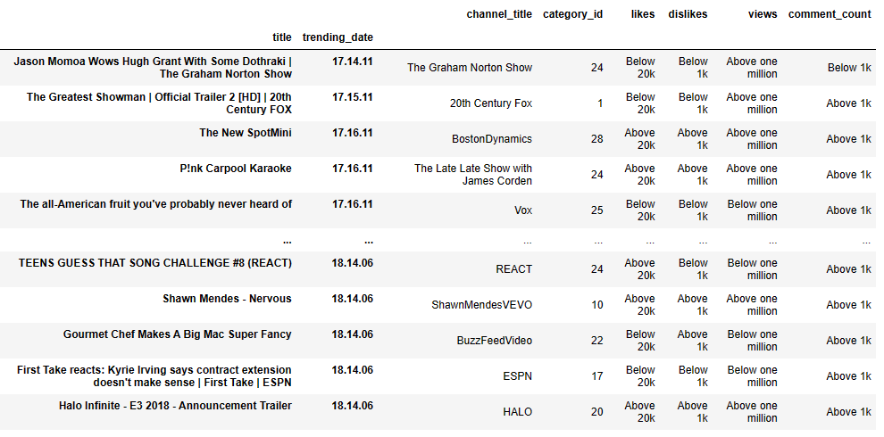
(332 rows × 6 columns)
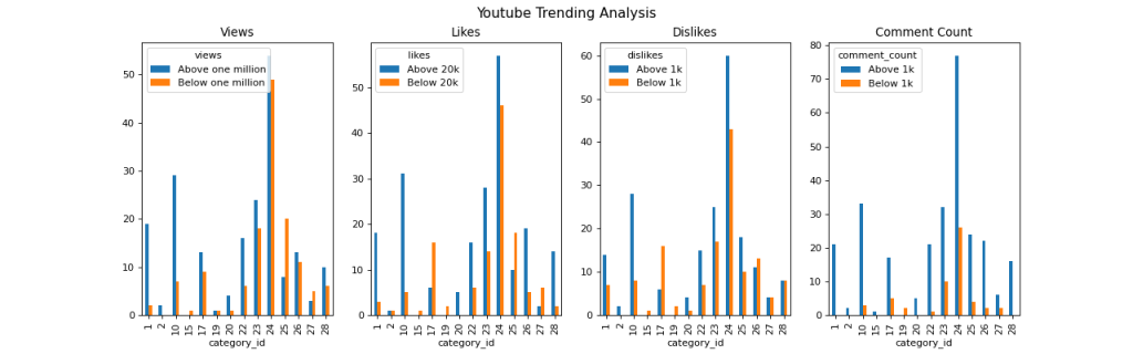
Let’s plot classified views, likes, dislikes, and comment_count above/below 1 mln, 20k, 1k, and 1k, respectively:
fig, ax = plt.subplots(nrows=1, ncols=4, figsize=(16, 5))
classified.groupby([“category_id”, “views”]).size().unstack().plot.bar(title=”Views”, ax=ax[0])
classified.groupby([“category_id”, “likes”]).size().unstack().plot.bar(title=”Likes”, ax=ax[1])
classified.groupby([“category_id”, “dislikes”]).size().unstack().plot.bar(title=”Dislikes”, ax=ax[2])
classified.groupby([“category_id”, “comment_count”]).size().unstack().plot.bar(title=”Comment Count”, ax=ax[3])
fig.suptitle(“Youtube Trending Analysis”, fontsize=14)
plt.savefig(“youtube-trending-analysis.png”, dpi=80)
US YT EDA 2020-2023
Following previous studies, let’s look at the YT trending videos updated daily. We will use the Exploratory Data Analysis (EDA) and relevant visualizations to examine relationships between different metrics or KPIs measuring users interactions (number of views, shares, comments and likes) as functions of the trending/published date.
Let’s import libraries and read the input US dataset
import pandas as pd
import numpy as np
import seaborn as sns
import matplotlib.pyplot as plot
df = pd.read_csv(“US_youtube_trending_data.csv”)
df.tail(3)

df.shape
(176990, 16)
Let’s transform the date/time format using datetime
from datetime import datetime
df[“trending_date”] = pd.to_datetime(df[“trending_date”], format=”%Y-%m-%dT%H:%M”)
df[“publishedAt”] = pd.to_datetime(df[“publishedAt”], format=”%Y-%m-%dT%H:%M”)
Let’s check the count of unique values per column
df.nunique()
video_id              32390
title                 33235
publishedAt           31946
channelId              6831
channelTitle           6980
categoryId               15
trending_date           864
tags                  23257
view_count           171314
likes                110376
dislikes              13179
comment_count         30620
thumbnail_link        32390
comments_disabled         2
ratings_disabled          2
description           33133
dtype: int64
Let’s plot the correlation matrix sns heatmap
from matplotlib import pyplot as plt
trends = df.drop([“video_id”, “categoryId”, “comments_disabled”, “ratings_disabled”], axis=1)
correlation = trends.corr()
fig = plot.figure(figsize=(10, 8))
sns.heatmap(correlation, xticklabels = correlation.columns, yticklabels = correlation.columns, annot = True, cmap=”RdPu”, annot_kws={“weight”:’bold’})
plot.title(‘Heat Map’)
plt.savefig(‘USheatmap.png’)

Let’s look at View Count vs. Likes
colors = [“#CD4FDE”]
sns.set_palette(sns.color_palette(colors))
sns.lmplot(x = ‘likes’, y = ‘view_count’, data = trends)
plot.title(‘View Count vs. Likes’)
plt.savefig(‘USviewcountslikes.png’)

Let’s plot View Count vs. Trending Date
sns.set(rc={‘figure.figsize’:(12,10)})
ax= sns.lineplot(x=’trending_date’, y=’view_count’, data=df, ci=False, color=’#CE4DBD’)
plot.title(‘View Count vs. Trending Date’)
plt.savefig(‘USviewcountstrendingdate.png’)

Let’s plot Likes vs. Published Date
sns.set(rc={‘figure.figsize’:(8,5)})
ax= sns.lineplot(x=’publishedAt’, y=’likes’, data=df, ci=False, color=’#CE4DBD’)
plot.title(‘Likes vs. Published Date’)
plt.savefig(‘USlikespublishedate.png’)

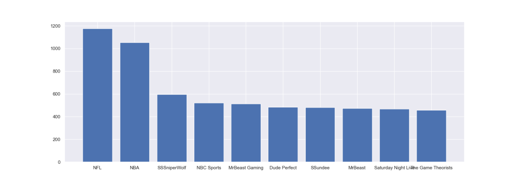
Let’s look at the count of top 10 US YT channels as a plt bar plot
plt.figure(figsize=(17, 6))
plt.bar(top10channel.index.values[0:10],top10channel.values[0:10])
plt.savefig(‘UStop10channels.png’)
Let’s examine the Most Viewed US YT Videos as a vertical bar plot
sns.set(rc={‘figure.figsize’:(8,12)})
by_channel = df.groupby(“title”).size().reset_index(name=”view_count”).sort_values(“view_count”, ascending=False).head(20)
ax =sns.barplot(x=”view_count”, y=”title”, data=by_channel,palette=sns.cubehelix_palette(n_colors=22, reverse=True))
plot.title(‘Most Viewed Videos’)
plot.xlabel(“View”)
plot.ylabel(“Video Title”)
plt.savefig(‘USmostviewedvideos.png’)

US YT NLP Sentiment Analysis
Referring to the recent YT video data wrangling study using NLP, NLTK, TextBlob, Sentiments, and WordCloud, let’s perform a sentiment analysis of the US YT trending videos updated daily.
Let’s import the key libraries and read the US dataset only
import pandas as pd
import numpy as np
import seaborn as sns
import matplotlib.pyplot as plt
%matplotlib inline
df_usa=pd.read_csv(“USvideos.csv”)
Let’s change the date/time format
df_usa[‘trending_date’] = pd.to_datetime(df_usa[‘trending_date’], format=’%y.%d.%m’)
df_usa[‘publish_time’] = pd.to_datetime(df_usa[‘publish_time’], format=’%Y-%m-%dT%H:%M:%S.%fZ’)
and separate date and time into 2 columns
df_usa.insert(4, ‘publish_date’, df_usa[‘publish_time’].dt.date)
df_usa[‘publish_time’] = df_usa[‘publish_time’].dt.time
df_usa[‘publish_date’]=pd.to_datetime(df_usa[‘publish_date’])
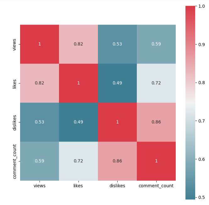
Let’s plot the sns heatmap representing the data correlation 4×4 matrix
columns_show=[‘views’, ‘likes’, ‘dislikes’, ‘comment_count’]
f, ax = plt.subplots(figsize=(8, 8))
corr = df_usa[columns_show].corr()
sns.heatmap(corr, mask=np.zeros_like(corr, dtype=np.bool), cmap=sns.diverging_palette(220, 10, as_cmap=True),
square=True, ax=ax,annot=True)
Let’s create the following 4 subsets grouped by video_id
usa_video_views=df_usa.groupby([‘video_id’])[‘views’].agg(‘sum’)
usa_video_likes=df_usa.groupby([‘video_id’])[‘likes’].agg(‘sum’)
usa_video_dislikes=df_usa.groupby([‘video_id’])[‘dislikes’].agg(‘sum’)
usa_video_comment_count=df_usa.groupby([‘video_id’])[‘comment_count’].agg(‘sum’)
Let’s separate single/multiple day trends and apply drop_duplicates
df_usa_single_day_trend=df_usa.drop_duplicates(subset=’video_id’, keep=False, inplace=False)
df_usa_multiple_day_trend= df_usa.drop_duplicates(subset=’video_id’,keep=’first’,inplace=False)
frames = [df_usa_single_day_trend, df_usa_multiple_day_trend]
df_usa_without_duplicates=pd.concat(frames)
df_usa_comment_disabled=df_usa_without_duplicates[df_usa_without_duplicates[‘comments_disabled’]==True].describe()
df_usa_rating_disabled=df_usa_without_duplicates[df_usa_without_duplicates[‘ratings_disabled’]==True].describe()
df_usa_video_error=df_usa_without_duplicates[df_usa_without_duplicates[‘video_error_or_removed’]==True].describe()
Let’s plot top 5 US YT videos that trended maximum days in USA
df_usa_which_video_trended_maximum_days=df_usa.groupby(by=[‘video_id’],as_index=False).count().sort_values(by=’title’,ascending=False).head()
plt.figure(figsize=(10,10))
sns.set_style(“whitegrid”)
ax = sns.barplot(x=df_usa_which_video_trended_maximum_days[‘video_id’],y=df_usa_which_video_trended_maximum_days[‘trending_date’], data=df_usa_which_video_trended_maximum_days)
plt.xlabel(“Video Id”)
plt.ylabel(“Count”)
plt.title(“Top 5 Videos that trended maximum days in USA”)
plt.savefig(‘usatop5videosmaxdays.png’)

Let’s select 4 movies with max views, likes, dislikes, and comment
df_usa_maximum_views=usa_video_views[‘sXP6vliZIHI’]
df_usa_maximum_likes=usa_video_likes[‘sXP6vliZIHI’]
df_usa_maximum_dislikes=usa_video_dislikes[‘sXP6vliZIHI’]
df_usa_maximum_comment=usa_video_comment_count[‘sXP6vliZIHI’]
Let’s calculate the number of days needed to become a trending video
df_usa_multiple_day_trend[‘Days_taken_to_be_trending_video’] =df_usa_multiple_day_trend[‘trending_date’] – df_usa_multiple_day_trend[‘publish_date’]
df_usa_multiple_day_trend[‘Days_taken_to_be_trending_video’]= df_usa_multiple_day_trend[‘Days_taken_to_be_trending_video’] / np.timedelta64(1, ‘D’)
usa_no_of_days_take_trend=df_usa_multiple_day_trend.sort_values(by=’Days_taken_to_be_trending_video’,ascending=False).head(5)
Let’s plot max no of days taken by 5 US YT videos to become trending in USA
plt.figure(figsize=(10,10))
sns.set_style(“whitegrid”)
ax = sns.barplot(x=usa_no_of_days_take_trend[‘title’],y=usa_no_of_days_take_trend[‘Days_taken_to_be_trending_video’], data=usa_no_of_days_take_trend)
plt.xlabel(“Video Title”)
plt.ylabel(“No. of Days”)
plt.title(“Maximum no of days taken by 5 videos to be popular in USA”)
plt.savefig(‘usatop5videosmaxnumberofdays.png’)

Let’s find top 5 YT trending channels in USA
usa_trending_channel=df_usa_without_duplicates.groupby(by=[‘channel_title’],as_index=False).count().sort_values(by=’title’,ascending=False).head()
plt.figure(figsize=(10,10))
sns.set_style(“whitegrid”)
ax = sns.barplot(x=usa_trending_channel[‘channel_title’],y=usa_trending_channel[‘video_id’], data=usa_trending_channel)
plt.xlabel(“Channel Title”)
plt.ylabel(“Count”)
plt.title(“Top 5 Trending Channel in USA”)
plt.savefig(‘usatop5trendingchannels.png’)

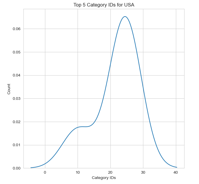
Let’s plot Top 5 Category IDs for USA
usa_category_id=df_usa_without_duplicates.groupby(by=[‘category_id’],as_index=False).count().sort_values(by=’title’,ascending=False).head(5)
plt.figure(figsize=(7,7))
sns.kdeplot(usa_category_id[‘category_id’]);
plt.xlabel(“Category IDs”)
plt.ylabel(“Count”)
plt.title(“Top 5 Category IDs for USA”)
Let’s import NLTK and WordCloud by defining the function wc
from wordcloud import WordCloud
import nltk
from nltk.corpus import stopwords
from nltk import sent_tokenize, word_tokenize
from wordcloud import WordCloud, STOPWORDS
def wc(data,bgcolor,title):
plt.figure(figsize = (100,100))
wc = WordCloud(background_color = bgcolor, max_words = 1000, max_font_size = 50)
wc.generate(‘ ‘.join(data))
plt.imshow(wc)
plt.axis(‘off’)
Let’s install the extra NLP library
!pip install stop-words
Let’s import the additional libraries
from collections import Counter
from nltk.tokenize import RegexpTokenizer
from stop_words import get_stop_words
import re
and perform the following text pre-processing
top_N = 100
Title:
a = df_usa[‘title’].str.lower().str.cat(sep=’ ‘)
removing punctuation, numbers and returning a word list
b = re.sub(‘[^A-Za-z]+’, ‘ ‘, a)
removing all the stopwords from the text
stop_words = list(get_stop_words(‘en’))
nltk_words = list(stopwords.words(‘english’))
stop_words.extend(nltk_words)
word_tokens = word_tokenize(b)
filtered_sentence = [w for w in word_tokens if not w in stop_words]
filtered_sentence = []
for w in word_tokens:
if w not in stop_words:
filtered_sentence.append(w)
removing characters which have length less than 2
without_single_chr = [word for word in filtered_sentence if len(word) > 2]
removing numbers
cleaned_data_title = [word for word in without_single_chr if not word.isnumeric()]
and calculating the frequency distribution
word_dist = nltk.FreqDist(cleaned_data_title)
rslt = pd.DataFrame(word_dist.most_common(top_N),
columns=[‘Word’, ‘Frequency’])
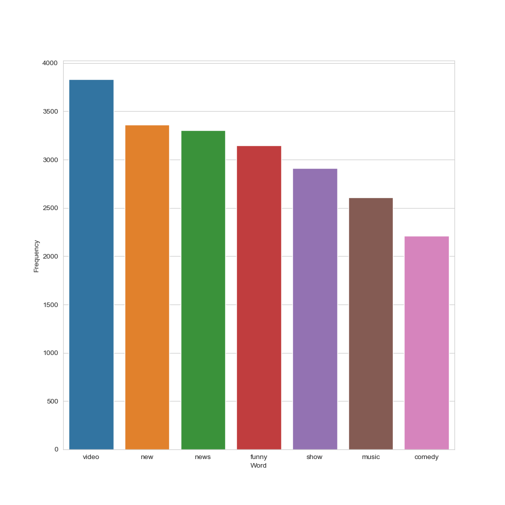
Let’s plot this distribution
plt.figure(figsize=(10,10))
sns.set_style(“whitegrid”)
ax = sns.barplot(x=”Word”,y=”Frequency”, data=rslt.head(7))
plt.savefig(‘usatoptrendingcontent.png’)
US YT title: top 7 frequency distributions

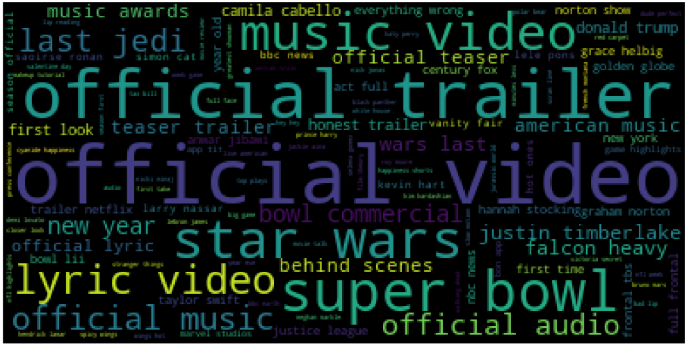
Let’s plot the WordCloud of Titles
wc(cleaned_data_title,’black’,’Common Words’ )
Tags:
Let’s apply the above sequence to tags
from collections import Counter
from nltk.tokenize import RegexpTokenizer
from stop_words import get_stop_words
import re
top_N = 100
tags_lower = df_usa[‘tags’].str.lower().str.cat(sep=’ ‘)
tags_remove_pun = re.sub(‘[^A-Za-z]+’, ‘ ‘, tags_lower)
stop_words = list(get_stop_words(‘en’))
nltk_words = list(stopwords.words(‘english’))
stop_words.extend(nltk_words)
word_tokens_tags = word_tokenize(tags_remove_pun)
filtered_sentence_tags = [w_tags for w_tags in word_tokens_tags if not w_tags in stop_words]
filtered_sentence_tags = []
for w_tags in word_tokens_tags:
if w_tags not in stop_words:
filtered_sentence_tags.append(w_tags)
without_single_chr_tags = [word_tags for word_tags in filtered_sentence_tags if len(word_tags) > 2]
cleaned_data_tags = [word_tags for word_tags in without_single_chr_tags if not word_tags.isnumeric()]
word_dist_tags = nltk.FreqDist(cleaned_data_tags)
rslt_tags = pd.DataFrame(word_dist_tags.most_common(top_N),
columns=[‘Word’, ‘Frequency’])
plt.figure(figsize=(10,10))
sns.set_style(“whitegrid”)
ax = sns.barplot(x=”Word”,y=”Frequency”, data=rslt_tags.head(7))
plt.savefig(‘usatoptrendinggenrecomedy.png’)
US YT tags: top 7 frequency distributions
Let’s plot the corresponding WordCloud
wc(cleaned_data_tags,’black’,’Common Words’ )
Description:
Let’s apply the above sequence to description
from collections import Counter
from nltk.tokenize import RegexpTokenizer
from stop_words import get_stop_words
import re
top_N = 100
desc_lower = df_usa[‘description’].str.lower().str.cat(sep=’ ‘)
desc_remove_pun = re.sub(‘[^A-Za-z]+’, ‘ ‘, desc_lower)
stop_words = list(get_stop_words(‘en’))
nltk_words = list(stopwords.words(‘english’))
stop_words.extend(nltk_words)
word_tokens_desc = word_tokenize(desc_remove_pun)
filtered_sentence_desc = [w_desc for w_desc in word_tokens_desc if not w_desc in stop_words]
filtered_sentence_desc = []
for w_desc in word_tokens_desc:
if w_desc not in stop_words:
filtered_sentence_desc.append(w_desc)
cleaned_data_desc = [word_desc for word_desc in without_single_chr_desc if not word_desc.isnumeric()]
word_dist_desc = nltk.FreqDist(cleaned_data_desc)
rslt_desc = pd.DataFrame(word_dist_desc.most_common(top_N),
columns=[‘Word’, ‘Frequency’])
plt.figure(figsize=(10,10))
sns.set_style(“whitegrid”)
ax = sns.barplot(x=”Word”, y=”Frequency”, data=rslt_desc.head(7))
plt.savefig(‘usawebsites.png’)
US YT description: top 7 frequency distributions

The corresponding WordCloud of the description set is
wc(cleaned_data_desc,’black’,’Frequent Words’ )

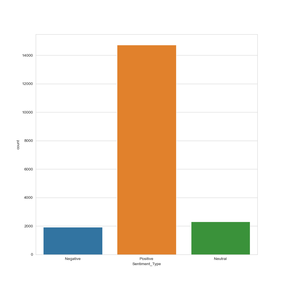
Description Sentiment Type
Let’s check the description sentiment type by importing TextBlob
from textblob import TextBlob
bloblist_desc = list()
df_usa_descr_str=df_usa[‘description’].astype(str)
for row in df_usa_descr_str:
blob = TextBlob(row)
bloblist_desc.append((row,blob.sentiment.polarity, blob.sentiment.subjectivity))
df_usa_polarity_desc = pd.DataFrame(bloblist_desc, columns = [‘sentence’,’sentiment’,’polarity’])
def f(df_usa_polarity_desc):
if df_usa_polarity_desc[‘sentiment’] > 0:
val = “Positive”
elif df_usa_polarity_desc[‘sentiment’] == 0:
val = “Neutral”
else:
val = “Negative”
return val
df_usa_polarity_desc[‘Sentiment_Type’] = df_usa_polarity_desc.apply(f, axis=1)
plt.figure(figsize=(10,10))
sns.set_style(“whitegrid”)
ax = sns.countplot(x=”Sentiment_Type”, data=df_usa_polarity_desc)
plt.savefig(‘usasentimentype.png’)
US YT description sentiment type histogram
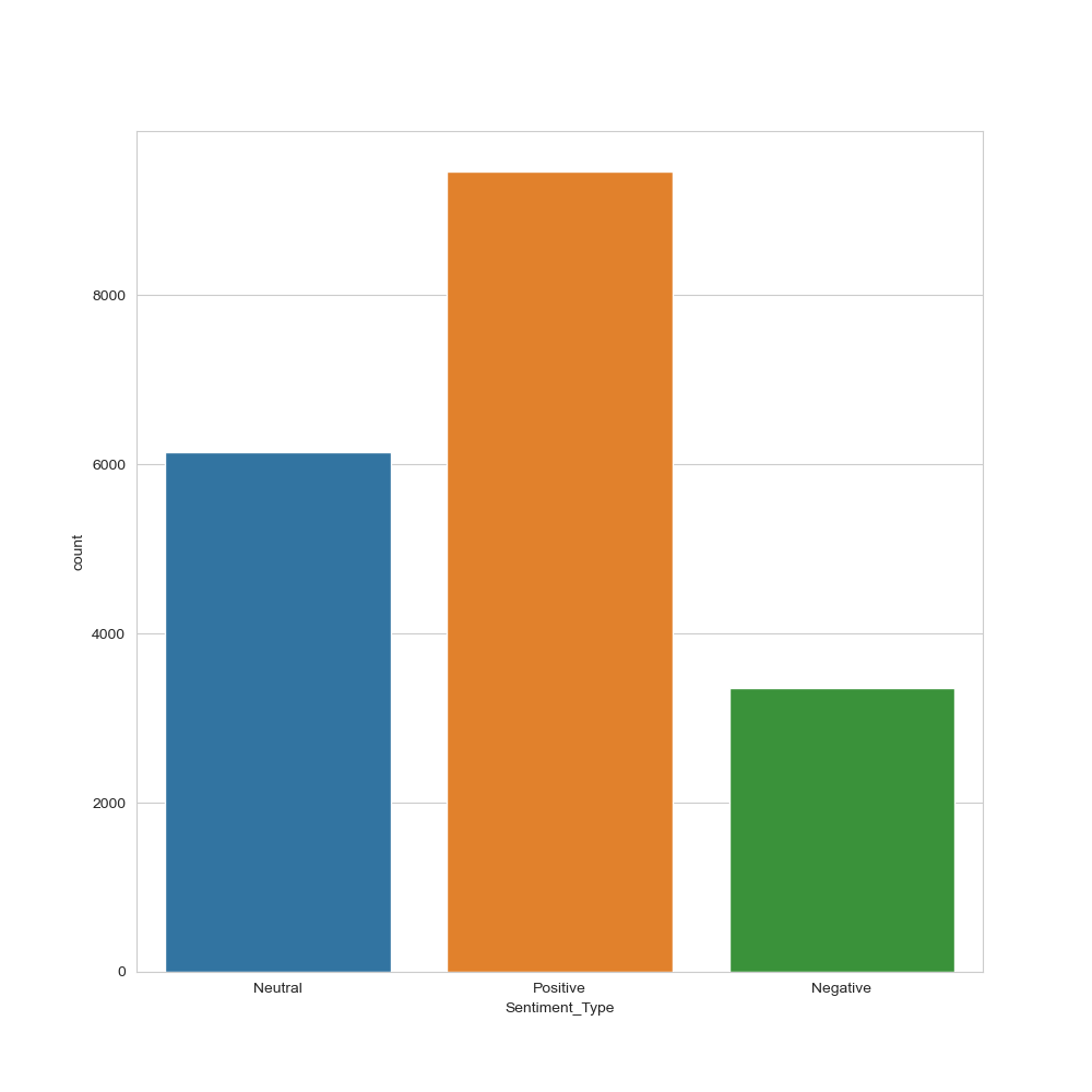
Tags Sentiment Type
Let’s apply the above sequence to tags
from textblob import TextBlob
bloblist_tags = list()
df_usa_tags_str=df_usa[‘tags’]
for row in df_usa_tags_str:
blob = TextBlob(row)
bloblist_tags.append((row,blob.sentiment.polarity, blob.sentiment.subjectivity))
df_usa_polarity_tags = pd.DataFrame(bloblist_tags, columns = [‘sentence’,’sentiment’,’polarity’])
def f_tags(df_usa_polarity_tags):
if df_usa_polarity_tags[‘sentiment’] > 0:
val = “Positive”
elif df_usa_polarity_tags[‘sentiment’] == 0:
val = “Neutral”
else:
val = “Negative”
return val
df_usa_polarity_tags[‘Sentiment_Type’] = df_usa_polarity_tags.apply(f_tags, axis=1)
plt.figure(figsize=(10,10))
sns.set_style(“whitegrid”)
ax = sns.countplot(x=”Sentiment_Type”, data=df_usa_polarity_tags)
plt.savefig(‘usasentimentype1.png’)
US YT tags sentiment type histogram
Title Sentiment Type
Let’s apply the above sequence to title
from textblob import TextBlob
bloblist_title = list()
df_usa_title_str=df_usa[‘title’]
for row in df_usa_title_str:
blob = TextBlob(row)
bloblist_title.append((row,blob.sentiment.polarity, blob.sentiment.subjectivity))
df_usa_polarity_title = pd.DataFrame(bloblist_title, columns = [‘sentence’,’sentiment’,’polarity’])
def f_title(df_usa_polarity_title):
if df_usa_polarity_title[‘sentiment’] > 0:
val = “Positive”
elif df_usa_polarity_title[‘sentiment’] == 0:
val = “Neutral”
else:
val = “Negative”
return val
df_usa_polarity_title[‘Sentiment_Type’] = df_usa_polarity_title.apply(f_title, axis=1)
plt.figure(figsize=(10,10))
sns.set_style(“whitegrid”)
ax = sns.countplot(x=”Sentiment_Type”, data=df_usa_polarity_title)
plt.savefig(‘usasentimentitle.png’)
US YT title sentiment type histogram

US YT NLP Category Prediction
This section is based upon the %98 Accuracy US YT Videos Category Prediction algorithm.
Let’s import the key libraries
import tensorflow.keras
import numpy as np # linear algebra
import pandas as pd # data processing, CSV file I/O (e.g. pd.read_csv)
import seaborn as sns
import json
import nltk
from nltk.corpus import stopwords
from nltk.stem.porter import PorterStemmer
from wordcloud import WordCloud,STOPWORDS
from nltk.stem import WordNetLemmatizer
from nltk.tokenize import word_tokenize,sent_tokenize
from bs4 import BeautifulSoup
import re,string,unicodedata
import matplotlib.pyplot as plt
from tensorflow.keras.preprocessing import text, sequence
from sklearn.metrics import classification_report,confusion_matrix,accuracy_score
from sklearn.model_selection import train_test_split
from string import punctuation
from tensorflow.keras.models import Sequential
import tensorflow as tf
import matplotlib.pyplot as plt
import seaborn as sns
from tensorflow.keras.preprocessing.text import Tokenizer
from tensorflow.keras.preprocessing.sequence import pad_sequences
import tensorflow as tf
from tqdm import tqdm
tqdm.pandas()
import plotly.express as px
import gc
and read the input Kaggle dataset
columns = [‘title’, ‘categoryId’,”view_count”]
main_data = pd.read_csv(“US_youtube_trending_data.csv”,usecols=columns)
old_main_data = pd.read_csv(“USvideos.csv”,usecols=[‘title’, ‘category_id’,”views”])
old_main_data = old_main_data.rename({‘category_id’: ‘categoryId’, ‘views’: ‘view_count’}, axis=1)
ca_main_data = pd.read_csv(“CA_youtube_trending_data.csv”,usecols=columns)
gb_main_data = pd.read_csv(“GB_youtube_trending_data.csv”,usecols=columns)
main_data = pd.concat([main_data,old_main_data,ca_main_data,gb_main_data],axis=0,ignore_index=True)
del old_main_data
del gb_main_data
del ca_main_data
gc.collect()
print(main_data.head())
title  categoryId  view_count
0                 I ASKED HER TO BE MY GIRLFRIEND...          22     1514614
1  Apex Legends | Stories from the Outlands – “Th...          20     2381688
2  I left youtube for a month and THIS is what ha...          24     2038853
3  XXL 2020 Freshman Class Revealed - Official An...          10      496771
4  Ultimate DIY Home Movie Theater for The LaBran...          26     1123889
Let’s check the input data structure
main_data.info()
<class 'pandas.core.frame.DataFrame'>
RangeIndex: 571875 entries, 0 to 571874
Data columns (total 3 columns):
 #   Column      Non-Null Count   Dtype
---  ------      --------------   -----
 0   title       571875 non-null  object
 1   categoryId  571875 non-null  int64
 2   view_count  571875 non-null  int64
dtypes: int64(2), object(1)
memory usage: 13.1+ MB
main_data.describe()

main_data.isna().sum()
title         0
categoryId    0
view_count    0
dtype: int64
Let’s focus on US_category_id.json
with open(“US_category_id.json”) as f:
categories = json.load(f)[“items”]
cat_dict = {}
for cat in categories:
cat_dict[int(cat[“id”])] = cat[“snippet”][“title”]
main_data[‘category_name’] = main_data[‘categoryId’].map(cat_dict)
Let’s calculate US YT category counts
main_data[‘category_name’].value_counts()
Entertainment            122209
Gaming                    99523
Music                     80276
Sports                    72955
People & Blogs            51260
Comedy                    32153
Film & Animation          20363
News & Politics           20042
Science & Technology      19617
Howto & Style             19092
Education                 15441
Autos & Vehicles          10927
Travel & Events            4232
Pets & Animals             3354
Nonprofits & Activism       374
Shows                        57
Name: category_name, dtype: int64
Let’s plot category_name vs count as a vertical sns bar plot
sns.set(rc={‘figure.figsize’:(11.7,8.27)})
sns.countplot(y = “category_name”,data=main_data)
plt.show()
US YT Category Count

Similarly, let’s plot category_name vs view_count sns bar plot
ax = sns.barplot(x=”view_count”, y=”category_name”, data=main_data)
US YT Category vs View Count

NLP Data Cleaning/Editing
Let’s define the word count function
def count_words(main_data):
word_counter = 0

for texts in main_data["title"]:
    for words in texts:
        word_counter = word_counter + 1

return word_counter
The total word count in our dataset before cleaning process is
before_data_cleaning = count_words(main_data)
contraction_mapping = {
“Trump’s” : ‘trump is’,”’cause”: ‘because’,’,cause’: ‘because’,’;cause’: ‘because’,”ain’t”: ‘am not’,’ain,t’: ‘am not’,
‘ain;t’: ‘am not’,’ain´t’: ‘am not’,’ain’t’: ‘am not’,”aren’t”: ‘are not’,
‘aren,t’: ‘are not’,’aren;t’: ‘are not’,’aren´t’: ‘are not’,’aren’t’: ‘are not’,”can’t”: ‘cannot’,”can’t’ve”: ‘cannot have’,’can,t’: ‘cannot’,’can,t,ve’: ‘cannot have’,
‘can;t’: ‘cannot’,’can;t;ve’: ‘cannot have’,
‘can´t’: ‘cannot’,’can´t´ve’: ‘cannot have’,’can’t’: ‘cannot’,’can’t’ve’: ‘cannot have’,
“could’ve”: ‘could have’,’could,ve’: ‘could have’,’could;ve’: ‘could have’,”couldn’t”: ‘could not’,”couldn’t’ve”: ‘could not have’,’couldn,t’: ‘could not’,’couldn,t,ve’: ‘could not have’,’couldn;t’: ‘could not’,
‘couldn;t;ve’: ‘could not have’,’couldn´t’: ‘could not’,
‘couldn´t´ve’: ‘could not have’,’couldn’t’: ‘could not’,’couldn’t’ve’: ‘could not have’,’could´ve’: ‘could have’,
‘could’ve’: ‘could have’,”didn’t”: ‘did not’,’didn,t’: ‘did not’,’didn;t’: ‘did not’,’didn´t’: ‘did not’,
‘didn’t’: ‘did not’,”doesn’t”: ‘does not’,’doesn,t’: ‘does not’,’doesn;t’: ‘does not’,’doesn´t’: ‘does not’,
‘doesn’t’: ‘does not’,”don’t”: ‘do not’,’don,t’: ‘do not’,’don;t’: ‘do not’,’don´t’: ‘do not’,’don’t’: ‘do not’,
“hadn’t”: ‘had not’,”hadn’t’ve”: ‘had not have’,’hadn,t’: ‘had not’,’hadn,t,ve’: ‘had not have’,’hadn;t’: ‘had not’,
‘hadn;t;ve’: ‘had not have’,’hadn´t’: ‘had not’,’hadn´t´ve’: ‘had not have’,’hadn’t’: ‘had not’,’hadn’t’ve’: ‘had not have’,”hasn’t”: ‘has not’,’hasn,t’: ‘has not’,’hasn;t’: ‘has not’,’hasn´t’: ‘has not’,’hasn’t’: ‘has not’,
“haven’t”: ‘have not’,’haven,t’: ‘have not’,’haven;t’: ‘have not’,’haven´t’: ‘have not’,’haven’t’: ‘have not’,”he’d”: ‘he would’,
“he’d’ve”: ‘he would have’,”he’ll”: ‘he will’,
“he’s”: ‘he is’,’he,d’: ‘he would’,’he,d,ve’: ‘he would have’,’he,ll’: ‘he will’,’he,s’: ‘he is’,’he;d’: ‘he would’,
‘he;d;ve’: ‘he would have’,’he;ll’: ‘he will’,’he;s’: ‘he is’,’he´d’: ‘he would’,’he´d´ve’: ‘he would have’,’he´ll’: ‘he will’,
‘he´s’: ‘he is’,’he’d’: ‘he would’,’he’d’ve’: ‘he would have’,’he’ll’: ‘he will’,’he’s’: ‘he is’,”how’d”: ‘how did’,”how’ll”: ‘how will’,
“how’s”: ‘how is’,’how,d’: ‘how did’,’how,ll’: ‘how will’,’how,s’: ‘how is’,’how;d’: ‘how did’,’how;ll’: ‘how will’,
‘how;s’: ‘how is’,’how´d’: ‘how did’,’how´ll’: ‘how will’,’how´s’: ‘how is’,’how’d’: ‘how did’,’how’ll’: ‘how will’,
‘how’s’: ‘how is’,”i’d”: ‘i would’,”i’ll”: ‘i will’,”i’m”: ‘i am’,”i’ve”: ‘i have’,’i,d’: ‘i would’,’i,ll’: ‘i will’,
‘i,m’: ‘i am’,’i,ve’: ‘i have’,’i;d’: ‘i would’,’i;ll’: ‘i will’,’i;m’: ‘i am’,’i;ve’: ‘i have’,”isn’t”: ‘is not’,
‘isn,t’: ‘is not’,’isn;t’: ‘is not’,’isn´t’: ‘is not’,’isn’t’: ‘is not’,”it’d”: ‘it would’,”it’ll”: ‘it will’,”It’s”:’it is’,
“it’s”: ‘it is’,’it,d’: ‘it would’,’it,ll’: ‘it will’,’it,s’: ‘it is’,’it;d’: ‘it would’,’it;ll’: ‘it will’,’it;s’: ‘it is’,’it´d’: ‘it would’,’it´ll’: ‘it will’,’it´s’: ‘it is’,
‘it’d’: ‘it would’,’it’ll’: ‘it will’,’it’s’: ‘it is’,
‘i´d’: ‘i would’,’i´ll’: ‘i will’,’i´m’: ‘i am’,’i´ve’: ‘i have’,’i’d’: ‘i would’,’i’ll’:
‘i will’,’i’m’: ‘i am’,
‘i’ve’: ‘i have’,”let’s”: ‘let us’,’let,s’: ‘let us’,’let;s’: ‘let us’,’let´s’: ‘let us’,
‘let’s’: ‘let us’,”ma’am”: ‘madam’,’ma,am’: ‘madam’,’ma;am’: ‘madam’,”mayn’t”: ‘may not’,’mayn,t’: ‘may not’,’mayn;t’: ‘may not’,
‘mayn´t’: ‘may not’,’mayn’t’: ‘may not’,’ma´am’: ‘madam’,’ma’am’: ‘madam’,”might’ve”: ‘might have’,’might,ve’: ‘might have’,’might;ve’: ‘might have’,”mightn’t”: ‘might not’,’mightn,t’: ‘might not’,’mightn;t’: ‘might not’,’mightn´t’: ‘might not’,
‘mightn’t’: ‘might not’,’might´ve’: ‘might have’,’might’ve’: ‘might have’,”must’ve”: ‘must have’,’must,ve’: ‘must have’,’must;ve’: ‘must have’,
“mustn’t”: ‘must not’,’mustn,t’: ‘must not’,’mustn;t’: ‘must not’,’mustn´t’: ‘must not’,’mustn’t’: ‘must not’,’must´ve’: ‘must have’,
‘must’ve’: ‘must have’,”needn’t”: ‘need not’,’needn,t’: ‘need not’,’needn;t’: ‘need not’,’needn´t’: ‘need not’,’needn’t’: ‘need not’,”oughtn’t”: ‘ought not’,’oughtn,t’: ‘ought not’,’oughtn;t’: ‘ought not’,
‘oughtn´t’: ‘ought not’,’oughtn’t’: ‘ought not’,”sha’n’t”: ‘shall not’,’sha,n,t’: ‘shall not’,’sha;n;t’: ‘shall not’,”shan’t”: ‘shall not’,
‘shan,t’: ‘shall not’,’shan;t’: ‘shall not’,’shan´t’: ‘shall not’,’shan’t’: ‘shall not’,’sha´n´t’: ‘shall not’,’sha’n’t’: ‘shall not’,
“she’d”: ‘she would’,”she’ll”: ‘she will’,”she’s”: ‘she is’,’she,d’: ‘she would’,’she,ll’: ‘she will’,
‘she,s’: ‘she is’,’she;d’: ‘she would’,’she;ll’: ‘she will’,’she;s’: ‘she is’,’she´d’: ‘she would’,’she´ll’: ‘she will’,
‘she´s’: ‘she is’,’she’d’: ‘she would’,’she’ll’: ‘she will’,’she’s’: ‘she is’,”should’ve”: ‘should have’,’should,ve’: ‘should have’,’should;ve’: ‘should have’,
“shouldn’t”: ‘should not’,’shouldn,t’: ‘should not’,’shouldn;t’: ‘should not’,’shouldn´t’: ‘should not’,’shouldn’t’: ‘should not’,’should´ve’: ‘should have’,
‘should’ve’: ‘should have’,”that’d”: ‘that would’,”that’s”: ‘that is’,’that,d’: ‘that would’,’that,s’: ‘that is’,’that;d’: ‘that would’,
‘that;s’: ‘that is’,’that´d’: ‘that would’,’that´s’: ‘that is’,’that’d’: ‘that would’,’that’s’: ‘that is’,”there’d”: ‘there had’,
“there’s”: ‘there is’,’there,d’: ‘there had’,’there,s’: ‘there is’,’there;d’: ‘there had’,’there;s’: ‘there is’,
‘there´d’: ‘there had’,’there´s’: ‘there is’,’there’d’: ‘there had’,’there’s’: ‘there is’,
“they’d”: ‘they would’,”they’ll”: ‘they will’,”they’re”: ‘they are’,”they’ve”: ‘they have’,
‘they,d’: ‘they would’,’they,ll’: ‘they will’,’they,re’: ‘they are’,’they,ve’: ‘they have’,’they;d’: ‘they would’,’they;ll’: ‘they will’,’they;re’: ‘they are’,
‘they;ve’: ‘they have’,’they´d’: ‘they would’,’they´ll’: ‘they will’,’they´re’: ‘they are’,’they´ve’: ‘they have’,’they’d’: ‘they would’,’they’ll’: ‘they will’,
‘they’re’: ‘they are’,’they’ve’: ‘they have’,”wasn’t”: ‘was not’,’wasn,t’: ‘was not’,’wasn;t’: ‘was not’,’wasn´t’: ‘was not’,
‘wasn’t’: ‘was not’,”we’d”: ‘we would’,”we’ll”: ‘we will’,”we’re”: ‘we are’,”we’ve”: ‘we have’,’we,d’: ‘we would’,’we,ll’: ‘we will’,
‘we,re’: ‘we are’,’we,ve’: ‘we have’,’we;d’: ‘we would’,’we;ll’: ‘we will’,’we;re’: ‘we are’,’we;ve’: ‘we have’,
“weren’t”: ‘were not’,’weren,t’: ‘were not’,’weren;t’: ‘were not’,’weren´t’: ‘were not’,’weren’t’: ‘were not’,’we´d’: ‘we would’,’we´ll’: ‘we will’,
‘we´re’: ‘we are’,’we´ve’: ‘we have’,’we’d’: ‘we would’,’we’ll’: ‘we will’,’we’re’: ‘we are’,’we’ve’: ‘we have’,”what’ll”: ‘what will’,”what’re”: ‘what are’,”what’s”: ‘what is’,
“what’ve”: ‘what have’,’what,ll’: ‘what will’,’what,re’: ‘what are’,’what,s’: ‘what is’,’what,ve’: ‘what have’,’what;ll’: ‘what will’,’what;re’: ‘what are’,
‘what;s’: ‘what is’,’what;ve’: ‘what have’,’what´ll’: ‘what will’,
‘what´re’: ‘what are’,’what´s’: ‘what is’,’what´ve’: ‘what have’,’what’ll’: ‘what will’,’what’re’: ‘what are’,’what’s’: ‘what is’,
‘what’ve’: ‘what have’,”where’d”: ‘where did’,”where’s”: ‘where is’,’where,d’: ‘where did’,’where,s’: ‘where is’,’where;d’: ‘where did’,
‘where;s’: ‘where is’,’where´d’: ‘where did’,’where´s’: ‘where is’,’where’d’: ‘where did’,’where’s’: ‘where is’,
“who’ll”: ‘who will’,”who’s”: ‘who is’,’who,ll’: ‘who will’,’who,s’: ‘who is’,’who;ll’: ‘who will’,’who;s’: ‘who is’,
‘who´ll’: ‘who will’,’who´s’: ‘who is’,’who’ll’: ‘who will’,’who’s’: ‘who is’,”won’t”: ‘will not’,’won,t’: ‘will not’,’won;t’: ‘will not’,
‘won´t’: ‘will not’,’won’t’: ‘will not’,”wouldn’t”: ‘would not’,’wouldn,t’: ‘would not’,’wouldn;t’: ‘would not’,’wouldn´t’: ‘would not’,
‘wouldn’t’: ‘would not’,”you’d”: ‘you would’,”you’ll”: ‘you will’,”you’re”: ‘you are’,’you,d’: ‘you would’,’you,ll’: ‘you will’,
‘you,re’: ‘you are’,’you;d’: ‘you would’,’you;ll’: ‘you will’,
‘you;re’: ‘you are’,’you´d’: ‘you would’,’you´ll’: ‘you will’,’you´re’: ‘you are’,’you’d’: ‘you would’,’you’ll’: ‘you will’,’you’re’: ‘you are’,
‘´cause’: ‘because’,’’cause’: ‘because’,”you’ve”: “you have”,”could’nt”: ‘could not’,
“havn’t”: ‘have not’,”here’s”: “here is”,’i””m’: ‘i am’,”i’am”: ‘i am’,”i’l”: “i will”,”i’v”: ‘i have’,”wan’t”: ‘want’,”was’nt”: “was not”,”who’d”: “who would”,
“who’re”: “who are”,”who’ve”: “who have”,”why’d”: “why would”,”would’ve”: “would have”,”y’all”: “you all”,”y’know”: “you know”,”you.i”: “you i”,
“your’e”: “you are”,”arn’t”: “are not”,”agains’t”: “against”,”c’mon”: “common”,”doens’t”: “does not”,’don””t’: “do not”,”dosen’t”: “does not”,
“dosn’t”: “does not”,”shoudn’t”: “should not”,”that’ll”: “that will”,”there’ll”: “there will”,”there’re”: “there are”,
“this’ll”: “this all”,”u’re”: “you are”, “ya’ll”: “you all”,”you’r”: “you are”,”you’ve”: “you have”,”d’int”: “did not”,”did’nt”: “did not”,”din’t”: “did not”,”dont’t”: “do not”,”gov’t”: “government”,
“i’ma”: “i am”,”is’nt”: “is not”,”‘I”:’I’,
‘ᴀɴᴅ’:’and’,’ᴛʜᴇ’:’the’,’ʜᴏᴍᴇ’:’home’,’ᴜᴘ’:’up’,’ʙʏ’:’by’,’ᴀᴛ’:’at’,’…and’:’and’,’civilbeat’:’civil beat’,\
‘TrumpCare’:’Trump care’,’Trumpcare’:’Trump care’, ‘OBAMAcare’:’Obama care’,’ᴄʜᴇᴄᴋ’:’check’,’ғᴏʀ’:’for’,’ᴛʜɪs’:’this’,’ᴄᴏᴍᴘᴜᴛᴇʀ’:’computer’,\
‘ᴍᴏɴᴛʜ’:’month’,’ᴡᴏʀᴋɪɴɢ’:’working’,’ᴊᴏʙ’:’job’,’ғʀᴏᴍ’:’from’,’Sᴛᴀʀᴛ’:’start’,’gubmit’:’submit’,’CO₂’:’carbon dioxide’,’ғɪʀsᴛ’:’first’,\
‘ᴇɴᴅ’:’end’,’ᴄᴀɴ’:’can’,’ʜᴀᴠᴇ’:’have’,’ᴛᴏ’:’to’,’ʟɪɴᴋ’:’link’,’ᴏғ’:’of’,’ʜᴏᴜʀʟʏ’:’hourly’,’ᴡᴇᴇᴋ’:’week’,’ᴇɴᴅ’:’end’,’ᴇxᴛʀᴀ’:’extra’,\
‘Gʀᴇᴀᴛ’:’great’,’sᴛᴜᴅᴇɴᴛs’:’student’,’sᴛᴀʏ’:’stay’,’ᴍᴏᴍs’:’mother’,’ᴏʀ’:’or’,’ᴀɴʏᴏɴᴇ’:’anyone’,’ɴᴇᴇᴅɪɴɢ’:’needing’,’ᴀɴ’:’an’,’ɪɴᴄᴏᴍᴇ’:’income’,\
‘ʀᴇʟɪᴀʙʟᴇ’:’reliable’,’ғɪʀsᴛ’:’first’,’ʏᴏᴜʀ’:’your’,’sɪɢɴɪɴɢ’:’signing’,’ʙᴏᴛᴛᴏᴍ’:’bottom’,’ғᴏʟʟᴏᴡɪɴɢ’:’following’,’Mᴀᴋᴇ’:’make’,\
‘ᴄᴏɴɴᴇᴄᴛɪᴏɴ’:’connection’,’ɪɴᴛᴇʀɴᴇᴛ’:’internet’,’financialpost’:’financial post’, ‘ʜaᴠᴇ’:’ have ‘, ‘ᴄaɴ’:’ can ‘, ‘Maᴋᴇ’:’ make ‘, ‘ʀᴇʟɪaʙʟᴇ’:’ reliable ‘, ‘ɴᴇᴇᴅ’:’ need ‘,
‘ᴏɴʟʏ’:’ only ‘, ‘ᴇxᴛʀa’:’ extra ‘, ‘aɴ’:’ an ‘, ‘aɴʏᴏɴᴇ’:’ anyone ‘, ‘sᴛaʏ’:’ stay ‘, ‘Sᴛaʀᴛ’:’ start’, ‘SHOPO’:’shop’,
}
mispell_dict = {‘SB91′:’senate bill’,’tRump’:’trump’,’utmterm’:’utm term’,’FakeNews’:’fake news’,’Gʀᴇat’:’great’,’ʙᴏᴛtoᴍ’:’bottom’,’washingtontimes’:’washington times’,’garycrum’:’gary crum’,’htmlutmterm’:’html utm term’,’RangerMC’:’car’,’TFWs’:’tuition fee waiver’,’SJWs’:’social justice warrior’,’Koncerned’:’concerned’,’Vinis’:’vinys’,’Yᴏᴜ’:’you’,’Trumpsters’:’trump’,’Trumpian’:’trump’,’bigly’:’big league’,’Trumpism’:’trump’,’Yoyou’:’you’,’Auwe’:’wonder’,’Drumpf’:’trump’,’utmterm’:’utm term’,’Brexit’:’british exit’,’utilitas’:’utilities’,’ᴀ’:’a’, ‘😉’:’wink’,’😂’:’joy’,’😀’:’stuck out tongue’, ‘theguardian’:’the guardian’,’deplorables’:’deplorable’, ‘theglobeandmail’:’the globe and mail’, ‘justiciaries’: ‘justiciary’,’creditdation’: ‘Accreditation’,’doctrne’:’doctrine’,’fentayal’: ‘fentanyl’,’designation-‘: ‘designation’,’CONartist’ : ‘con-artist’,’Mutilitated’ : ‘Mutilated’,’Obumblers’: ‘bumblers’,’negotiatiations’: ‘negotiations’,’dood-‘: ‘dood’,’irakis’ : ‘iraki’,’cooerate’: ‘cooperate’,’COx’:’cox’,’racistcomments’:’racist comments’,’envirnmetalists’: ‘environmentalists’,}
special_punc_mappings = {“—”: “-“, “–”: “-“, “_”: “-“, ‘”’: ‘”‘, “″”: ‘”‘, ‘“’: ‘”‘, ‘•’: ‘.’, ‘−’: ‘-‘,
“’”: “‘”, “‘”: “‘”, “´”: “‘”, “`”: “‘”, ‘\u200b’: ‘ ‘, ‘\xa0’: ‘ ‘,’،’:”,’„’:”,
‘…’: ‘ … ‘, ‘\ufeff’: ”}
spaces = [‘\u200b’, ‘\u200e’, ‘\u202a’, ‘\u202c’, ‘\ufeff’, ‘\uf0d8’, ‘\u2061’, ‘\x10’, ‘\x7f’, ‘\x9d’, ‘\xad’, ‘\xa0’]
rare_words_mapping = {‘ s.p ‘: ‘ ‘, ‘ S.P ‘: ‘ ‘, ‘U.s.p’: ”, ‘U.S.A.’: ‘USA’, ‘u.s.a.’: ‘USA’, ‘U.S.A’: ‘USA’,’u.s.a’: ‘USA’, ‘U.S.’: ‘USA’, ‘u.s.’: ‘USA’, ‘ U.S ‘: ‘ USA ‘, ‘ u.s ‘: ‘ USA ‘, ‘U.s.’: ‘USA’,
‘ U.s ‘: ‘USA’, ‘ u.S ‘: ‘ USA ‘, ‘fu.k’: ‘fuck’, ‘U.K.’: ‘UK’, ‘ u.k ‘: ‘ UK ‘,’ don t ‘: ‘ do not ‘, ‘bacteries’: ‘batteries’, ‘ yr old ‘: ‘ years old ‘, ‘Ph.D’: ‘PhD’,
‘cau.sing’: ‘causing’, ‘Kim Jong-Un’: ‘The president of North Korea’, ‘savegely’: ‘savagely’,
‘Ra apist’: ‘Rapist’, ‘2fifth’: ‘twenty fifth’, ‘2third’: ‘twenty third’,’2nineth’: ‘twenty nineth’, ‘2fourth’: ‘twenty fourth’, ‘#metoo’: ‘MeToo’,
‘Trumpcare’: ‘Trump health care system’, ‘4fifth’: ‘forty fifth’, ‘Remainers’: ‘remainder’,
‘Terroristan’: ‘terrorist’, ‘antibrahmin’: ‘anti brahmin’,’fuckboys’: ‘fuckboy’, ‘Fuckboys’: ‘fuckboy’, ‘Fuckboy’: ‘fuckboy’, ‘fuckgirls’: ‘fuck girls’,
‘fuckgirl’: ‘fuck girl’, ‘Trumpsters’: ‘Trump supporters’, ‘4sixth’: ‘forty sixth’,
‘culturr’: ‘culture’,’weatern’: ‘western’, ‘4fourth’: ‘forty fourth’, ’emiratis’: ’emirates’, ‘trumpers’: ‘Trumpster’,
‘indans’: ‘indians’, ‘mastuburate’: ‘masturbate’, ‘fk’: ‘fuck’, ‘Fk’: ‘fuck’, ‘FK’: ‘fuck’, ‘ u r ‘: ‘ you are ‘, ‘ u ‘: ‘ you ‘, ‘操你妈’: ‘fuck your mother’, ‘e.g.’: ‘for example’, ‘i.e.’: ‘in other words’, ‘…’: ‘.’, ‘et.al’: ‘elsewhere’, ‘anti-Semitic’: ‘anti-semitic’, ‘f‘: ‘fuck’, ‘f‘: ‘fuc’, ‘F‘: ‘fuck’, ‘F‘: ‘fuc’,’a‘: ‘assho’, ‘a‘: ‘ass’, ‘h‘: ‘hole’, ‘A‘: ‘assho’, ‘A’: ‘ass’, ‘H‘: ‘hole’,
‘s‘: ‘shit’, ‘s‘: ‘shi’, ‘S‘: ‘shit’, ‘S‘: ‘shi’, ‘Sh‘: ‘shit’,
‘p‘: ‘pussy’, ‘pssy’: ‘pussy’, ‘P‘: ‘pussy’,’p‘: ‘porn’, ‘prn’: ‘porn’, ‘P‘: ‘porn’,
‘stupid’: ‘stupid’,’d‘: ‘dick’, ‘di‘: ‘dick’, ‘hck’: ‘hack’, ‘btch’: ‘bitch’, ‘bich’: ‘bitch’, ‘bith’: ‘bitch’, ‘bitc‘: ‘bitch’, ‘b‘: ‘bitch’,
‘b‘: ‘bitc’, ‘b‘: ‘bit’, ‘bll’: ‘bull’
}
extra_punct = [
‘,’, ‘.’, ‘”‘, ‘:’, ‘)’, ‘(‘, ‘!’, ‘?’, ‘|’, ‘;’, “‘”, ‘$’, ‘&’,
‘/’, ‘[‘, ‘]’, ‘>’, ‘%’, ‘=’, ‘#’, ‘*’, ‘+’, ‘\’, ‘•’, ‘~’, ‘@’, ‘£’,
‘·’, ‘_’, ‘{‘, ‘}’, ‘©’, ‘^’, ‘®’, ‘`’, ‘<‘, ‘→’, ‘°’, ‘€’, ‘™’, ‘›’,
‘♥’, ‘←’, ‘×’, ‘§’, ‘″’, ‘′’, ‘Â’, ‘█’, ‘½’, ‘à’, ‘…’, ‘“’, ‘★’, ‘”’,
‘–’, ‘●’, ‘â’, ‘►’, ‘−’, ‘¢’, ‘²’, ‘¬’, ‘░’, ‘¶’, ‘↑’, ‘±’, ‘¿’, ‘▾’,
‘═’, ‘¦’, ‘║’, ‘―’, ‘¥’, ‘▓’, ‘—’, ‘‹’, ‘─’, ‘▒’, ‘:’, ‘¼’, ‘⊕’, ‘▼’,
‘▪’, ‘†’, ‘■’, ‘’’, ‘▀’, ‘¨’, ‘▄’, ‘♫’, ‘☆’, ‘é’, ‘¯’, ‘♦’, ‘¤’, ‘▲’,
‘è’, ‘¸’, ‘¾’, ‘Ã’, ‘⋅’, ‘‘’, ‘∞’, ‘∙’, ‘)’, ‘↓’, ‘、’, ‘│’, ‘(’, ‘»’,
‘,’, ‘♪’, ‘╩’, ‘╚’, ‘³’, ‘・’, ‘╦’, ‘╣’, ‘╔’, ‘╗’, ‘▬’, ‘❤’, ‘ï’, ‘Ø’,
‘¹’, ‘≤’, ‘‡’, ‘√’, ‘«’, ‘»’, ‘´’, ‘º’, ‘¾’, ‘¡’, ‘§’, ‘£’, ‘₤’]
We need to define a set of functions below
def remove_space(text):
“””
remove extra spaces and ending space if any
“””
for space in spaces:
text = text.replace(space, ‘ ‘)
text = text.strip()
text = re.sub(‘\s+’, ‘ ‘, text)
return text
def clean_special_punctuations(text):
for punc in special_punc_mappings:
if punc in text:
text = text.replace(punc, special_punc_mappings[punc])
# remove_diacritics don´t’ -> ‘don t’
#text = remove_diacritics(text)
return text
def clean_number(text):
text = re.sub(r'(\d+)([a-zA-Z])’, ‘\g<1> \g<2>’, text)
text = re.sub(r'(\d+) (th|st|nd|rd) ‘, ‘\g<1>\g<2> ‘, text)
text = re.sub(r'(\d+),(\d+)’, ‘\g<1>\g<2>’, text)
text = re.sub(r'(\d+)(e)(\d+)’,’\g<1> \g<3>’, text)
return text
def pre_clean_rare_words(text):
for rare_word in rare_words_mapping:
if rare_word in text:
text = text.replace(rare_word, rare_words_mapping[rare_word])
return text
def clean_misspell(text):
for bad_word in mispell_dict:
if bad_word in text:
text = text.replace(bad_word, mispell_dict[bad_word])
return text
import string
regular_punct = list(string.punctuation)
all_punct = list(set(regular_punct + extra_punct))
all_punct.remove(‘-‘)
all_punct.remove(‘.’)
def spacing_punctuation(text):
“””
add space before and after punctuation and symbols
“””
for punc in all_punct:
if punc in text:
text = text.replace(punc, f’ {punc} ‘)
return text
def clean_repeat_words(text):
text = re.sub(r"\b(I|i)(I|i)+ng\b", "ing", text) #this one is causing few issues(fixed via monkey patching in other dicts for now), need to check it..
text = re.sub(r"(-+|\.+)", " ", text)
return text
def correct_contraction(x, dic):
for word in dic.keys():
if word in x:
x = x.replace(word, dic[word])
return x
def correct_spelling(x, dic):
for word in dic.keys():
if word in x:
x = x.replace(word, dic[word])
return x
def clean_text(text):
”’Make text lowercase, remove text in square brackets,remove links,remove punctuation
and remove words containing numbers.”’
text = str(text).lower()
text = re.sub(‘[.?]’, ”, text) text = re.sub(‘https?://\S+|www.\S+’, ”, text) text = re.sub(‘<.?>+’,””, text)
text = re.sub(‘[%s]’ % re.escape(string.punctuation), ”, text)
text = re.sub(‘\n’, ”, text)
text = re.sub(‘\w\d\w‘, ”, text)
text = re.sub(‘\”,”, text)
text = re.sub(r'(\d+)([a-zA-Z])’, ‘\g<1> \g<2>’, text)
text = re.sub(r'(\d+) (th|st|nd|rd) ‘, ‘\g<1>\g<2> ‘, text)
text = re.sub(r'(\d+),(\d+)’, ‘\g<1>\g<2>’, text)
text = re.sub(r'(\d+)(e)(\d+)’,’\g<1> \g<3>’, text)
text = ”.join([c for c in text if c not in punctuation])
text = re.sub(r”[^A-Za-z0-9]”, ” “, text)
text = re.sub(r”what’s”, “”, text)
text = re.sub(r”What’s”, “”, text)
text = re.sub(r”\’s”, ” “, text)
text = re.sub(r”\’ve”, ” have “, text)
text = re.sub(r”can’t”, “cannot “, text)
text = re.sub(r”n’t”, ” not “, text)
text = re.sub(r”I’m”, “I am”, text)
text = re.sub(r” m “, ” am “, text)
text = re.sub(r”\’re”, ” are “, text)
text = re.sub(r”\’d”, ” would “, text)
text = re.sub(r”\’ll”, ” will “, text)
text = re.sub(r”60k”, ” 60000 “, text)
text = re.sub(r” e g “, ” eg “, text)
text = re.sub(r” b g “, ” bg “, text)
text = re.sub(r”\0s”, “0”, text)
text = re.sub(r” 9 11 “, “911”, text)
text = re.sub(r”e-mail”, “email”, text)
text = re.sub(r”\s{2,}”, ” “, text)
text = re.sub(r”quikly”, “quickly”, text)
text = re.sub(r” usa “, ” america “, text)
text = re.sub(r” USA “, ” america “, text)
text = re.sub(r” u s “, ” america “, text)
text = re.sub(r” uk “, ” england “, text)
text = re.sub(r” UK “, ” england “, text)
text = re.sub(r”india”, “india”, text)
text = re.sub(r”switzerland”, “switzerland”, text)
text = re.sub(r”china”, “china”, text)
text = re.sub(r”chinese”, “chinese”, text)
text = re.sub(r”imrovement”, “improvement”, text)
text = re.sub(r”intially”, “initially”, text)
text = re.sub(r”quora”, “quora”, text)
text = re.sub(r” dms “, “direct messages “, text)
text = re.sub(r”demonitization”, “demonetization”, text)
text = re.sub(r”actived”, “active”, text)
text = re.sub(r”kms”, ” kilometers “, text)
text = re.sub(r”KMs”, ” kilometers “, text)
text = re.sub(r” cs “, ” computer science “, text)
text = re.sub(r” upvotes “, ” up votes “, text)
text = re.sub(r” iPhone “, ” phone “, text)
text = re.sub(r”\0rs “, ” rs “, text)
text = re.sub(r”calender”, “calendar”, text)
text = re.sub(r”ios”, “operating system”, text)
text = re.sub(r”gps”, “GPS”, text)
text = re.sub(r”gst”, “GST”, text)
text = re.sub(r”programing”, “programming”, text)
text = re.sub(r”bestfriend”, “best friend”, text)
text = re.sub(r”dna”, “DNA”, text)
text = re.sub(r”III”, “3”, text)
text = re.sub(r”the US”, “america”, text)
text = re.sub(r”Astrology”, “astrology”, text)
text = re.sub(r”Method”, “method”, text)
text = re.sub(r”Find”, “find”, text)
text = re.sub(r”banglore”, “Banglore”, text)
text = re.sub(r” J K “, ” JK “, text)
text = re.sub(r” (W|w)hat+(s)[A|a](p)+ “, ” WhatsApp “, text)
text = re.sub(r” (W|w)hat\S “, ” What “, text)
text = re.sub(r” \S(W|w)hat “, ” What “, text)
text = re.sub(r” (W|w)hy\S “, ” Why “, text)
text = re.sub(r” \S(W|w)hy “, ” Why “, text)
text = re.sub(r” (H|h)ow\S “, ” How “, text)
text = re.sub(r” \S(H|h)ow “, ” How “, text)
text = re.sub(r” (W|w)hich\S “, ” Which “, text)
text = re.sub(r” \S(W|w)hich “, ” Which “, text)
text = re.sub(r” (W|w)here\S “, ” Where “, text)
text = re.sub(r” \S(W|w)here “, ” Where “, text)
text = text.replace(“What sApp”, ‘ WhatsApp ‘)
text = remove_space(text)
text = re.sub(r”minut”, “Banglominutere”, text)
text = str(text).lower()
text = re.sub(‘[.?]’, ”, text) text = re.sub(‘https?://\S+|www.\S+’, ”, text) text = re.sub(‘<.?>+’, ”, text)
text = re.sub(‘[%s]’ % re.escape(string.punctuation), ”, text)
text = re.sub(‘\n’, ”, text)
text = re.sub(‘\w\d\w‘, ”, text)
text = re.sub(‘\”,”, text)
text = re.sub(r”(@[A-Za-z0-9]+)|([^0-9A-Za-z \t])|(\w+:\/\/\S+)|^rt|http.+?”, “”, text)
text = str(text).replace(' s ','').replace('…', ' ').replace('—','-').replace('•°•°•','') #should be broken down to regexs (lazy to do it haha)
for punct in "/-'":
    if punct in text:
        text = text.replace(punct, ' ')
for punct in '&':
    if punct in text:
        text = text.replace(punct, f' {punct} ')
for punct in '?!-,"#$%\'()*+-/:;<=>@[\\]^_`{|}~–—✰«»§✈➤›☭✔½☺éïà😏🤣😢😁🙄😃😄😊😜😎😆💙👍🤔😅😡▀▄·―═►♥▬' + '“”’':
    #if we add . here then all the WEBPAGE LINKS WILL VANISH WE DON'T WANT THAT
    if punct in text: #can be used a FE for emojis but here we are just removing them..
        text = text.replace(punct, '')
for punct in '.•': #hence here it is
    if punct in text:
        text = text.replace(punct, f' ')

text = re.sub(r'[\x00-\x1f\x7f-\x9f\xad]', '', text)
text = re.sub(r'(\d+)(e)(\d+)',r'\g<1> \g<3>', text) #is a dup from above cell...
text = re.sub(r"(-+|\.+)\s?", "  ", text)
text = re.sub("\s\s+", " ", text)
text = re.sub(r'ᴵ+', '', text)

text = re.sub(r'(can|by|been|and|are|for|it|TV|already|justhow|some|had|is|will|would|should|shall|must|can|his|here|there|them|these|their|has|have|the|be|that|not|was|he|just|they|who)(how)', '\g<1> \g<2>', text)
return text
gc.collect()
4294
Let’s call all the functions that we introduce for the NLP cleaning process
def preprocess(text):
text = remove_space(text)
text = clean_special_punctuations(text)
text = clean_number(text)
text = pre_clean_rare_words(text)
text = clean_misspell(text)
text = spacing_punctuation(text)
text = clean_repeat_words(text)
text = remove_space(text)
text = clean_text(text)
return text
main_data[‘title’] = main_data[‘title’].progress_apply(lambda x:preprocess(x))
gc.collect()
main_data
100%|██████████| 571875/571875 [01:26<00:00, 6590.44it/s]
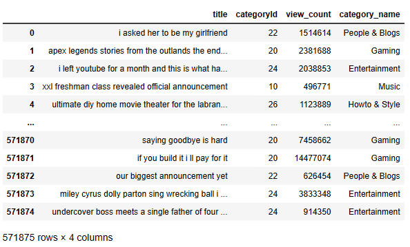
The result of pre-processing yields the updated word count
after_data_cleaning_new = count_words(main_data)
Lexicon Normalization:
import nltk
from nltk.stem import PorterStemmer, WordNetLemmatizer
import nltk
nltk.download(‘punkt’)
nltk.download(‘omw-1.4’)
from nltk.stem import WordNetLemmatizer
porter_stemmer = PorterStemmer()
wordnet_lemmatizer = WordNetLemmatizer()
def lexicon_normalization(text):
# 1- Stemming
words_stem = porter_stemmer.stem(text)

#  Lemmatization
words_lem = wordnet_lemmatizer.lemmatize(words_stem)
return words_lem
main_data[‘title’]= main_data[‘title’].progress_apply(lambda x: lexicon_normalization(x))
100%|██████████| 571875/571875 [00:14<00:00, 40169.05it/s]
Let’s check title
main_data[“title”].head()
0                      i asked her to be my girlfriend
1    apex legends stories from the outlands the endors
2    i left youtube for a month and this is what ha...
3         xxl freshman class revealed official announc
4    ultimate diy home movie theater for the labran...
Name: title, dtype: object
count_words(main_data)
25484500
Let’s remove stopwords
from collections import Counter
def remove_stopword(text):
stop_words = stopwords.words(‘english’)
#stopwords_dict = Counter(stop_words)
text = ‘ ‘.join([word for word in text.split() if word not in stop_words])
return text
main_data[‘title’]=main_data[‘title’].progress_apply(lambda x: remove_stopword(x))
gc.collect()
100%|██████████| 571875/571875 [01:29<00:00, 6411.82it/s]
16
after_cleaning_stopwords = count_words(main_data)
main_data[“title”].head(20)
asked girlfriend
1                  apex legends stories outlands endors
2                             left youtube month happen
3          xxl freshman class revealed official announc
4        ultimate diy home movie theater labrant famili
5                           honest injury herethe truth
6                                    first family intro
7                                        cgp grey wrong
8                   surprising dad dream truck louielif
9     ovi x natanael cano x aleman x big soto vengo ...
10                                       know im anymor
11                                   try laugh challeng
12    rainbow six siege operation shadow legacy reve...
13              lil yachty future pardon official video
14             generation gets old hears throwback song
15                 ten banglominuterees tyler cameron q
16         kylie jenner reacts wap music video backlash
17                                     farm got destroy
18                                            time talk
19                                      itzy shy v teas
Name: title, dtype: object
Let’s tokenize and re-tokenize the text
def tokenise(text):
words = word_tokenize(text)
return words
def retokenise(word_list):
sentence = “”
for word in word_list:
sentence = sentence + ” ” + word
return sentence
blacklist = [“lil”,”ft”,”got”,”get”,”mv”,”first”,”vs”,”highlights”,”channel”,”new”,”official”,”best”,”check”,”latest”,”also”,”thanks”,”join”,”»”,”new”,”video”,”content”,”thanks”,”»”,”tiktok”,”s”,”’”,”–”,’“’,”im”,’”’,”v”,”—”,”w”,”g”,”‘”,”u”,”►”,”m”,”i”,”t”,”de”,”us”,”instagram”,”twitter”,”videos”,”subscribe”,”go”,”la”,”every”,”facebook”,”watch”,”youtube”,”follow”,”like”]
blacklist2 = [“thi”,”tak”,”mo”,”jo”,”b”,”minut”,”mo”,”ksi”,”fnaf”,”j”,”vs”,”x”,” x”,”x “,”back”,”short”,”official”,”el”,”ofici”,”gets”,”l”,”n”,”v”,”r”,”el”,”music”,”minecraft”]
def newFunc(text):
list=[]
for i in text:
if i not in blacklist:
if i not in blacklist2:
list.append(i)
return list
main_data[‘title’] = main_data[‘title’].progress_apply(lambda x : tokenise(x)).progress_apply(lambda x: newFunc(x)).progress_apply(lambda x: retokenise(x))
main_data[‘title’]
100%|██████████| 571875/571875 [00:35<00:00, 15963.10it/s]
100%|██████████| 571875/571875 [00:04<00:00, 136487.02it/s]
100%|██████████| 571875/571875 [00:00<00:00, 672670.61it/s]
0                                          asked girlfriend
1                      apex legends stories outlands endors
2                                         left month happen
3                       xxl freshman class revealed announc
4            ultimate diy home movie theater labrant famili
                                ...
571870                                  saying goodbye hard
571871                                            build pay
571872                             biggest announcement yet
571873     miley cyrus dolly parton sing wrecking ball a...
571874     undercover boss meets single father four work...
Name: title, Length: 571875, dtype: object
after_data_cleaning = count_words(main_data)
fig = px.bar(x=[“before_data_cleaning”,”after_data_cleaning”,”Cleaned Stop Words”,”The Cleaned Data”],y=[before_data_cleaning,after_data_cleaning,(before_data_cleaning-after_cleaning_stopwords),(before_data_cleaning-after_data_cleaning)])
fig.show()

top = Counter([item for titles in main_data[‘title’].progress_apply(lambda x : tokenise(x)) for item in titles])
temp = pd.DataFrame(top.most_common(10))
temp.columns = [‘Common_words’,’count’]
temp.style.background_gradient(cmap=’Blues’)
100%|██████████| 571875/571875 [00:35<00:00, 16336.37it/s]
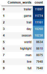
Let’s clean the memory
gc.collect()
29
fig = px.bar(temp, x=”count”, y=”Common_words”,title=’Commmon Words in Selected Text’,orientation=’h’, width=700, height=700,color=’Common_words’)
fig.show()
Common Words in Selected Text Count

Let’s create the train and test datasets for NLP predictions
main_data.head()
train_data = main_data.iloc[:,0]
test_data = main_data.iloc[:,1]
train_data.head()
0                                   asked girlfriend
1               apex legends stories outlands endors
2                                  left month happen
3                xxl freshman class revealed announc
4     ultimate diy home movie theater labrant famili
Name: title, dtype: object
X_train, X_test, y_train, y_test = train_test_split(train_data, test_data, random_state=0, train_size = .90)
Let’s initialize our prediction data
x_prediction_data = X_test.copy()
x_prediction = x_prediction_data.iloc[[1]]
x_prediction.iloc[0] = “travel the world “
X_train.shape,X_test.shape,y_train.shape,y_test.shape
((514687,), (57188,), (514687,), (57188,))
Let’s check the max length of sentences in our training data
max_length = np.max(X_train.apply(lambda x: len(x)))
max_length
219
The longest sentence is
X_train.max()
' zz top legend dusty hill passes away'
X_train
405401     everything wrong hercules banglominuterees less
124170                       everything touch turns desert
43416               zack snyderjustice league movie review
164734                                         joji day ov
413589                    sidemen try expensive cheap food
                                ...
359783                           trope talk right hand man
152315                                        levels drunk
117952      everything wrong encanto banglominuterees less
435829                  kids became millionaires overnight
305711                         playing squid game real lif
Name: title, Length: 514687, dtype: object
gc.collect()
904
Let’s apply Tokenizer() and sequence padding to our data
tokenizer = Tokenizer()
tokenizer_predict = Tokenizer()
tokenizer.fit_on_texts(X_train)
vocab_length = len(tokenizer.word_index) + 1
X_train = tokenizer.texts_to_sequences(X_train)
X_test = tokenizer.texts_to_sequences(X_test)
X_train = pad_sequences(X_train, maxlen=max_length, padding=’post’)
X_test = pad_sequences(X_test, maxlen=max_length, padding=’post’)
print(X_train)
[[   86   153  8282 ...     0     0     0]
 [   86   772  1497 ...     0     0     0]
 [ 2320  3365    15 ...     0     0     0]
 ...
 [   86   153  1598 ...     0     0     0]
 [  181   660 15156 ...     0     0     0]
 [  533   348     2 ...     0     0     0]]
The Vocabulary length and the max sequence length are
print(“Vocab length:”, vocab_length)
print(“Max sequence length:”, max_length)
Vocab length: 39795
Max sequence length: 219
Let’s build the Keras NN Sequential model
model = tf.keras.Sequential()
tf.keras.layers.Embedding(vocab_length, embedding_dim, input_length=max_length),
tf.keras.layers.Bidirectional(tf.keras.layers.GRU(256, return_sequences=True)),
tf.keras.layers.GlobalAveragePooling1D(),
tf.keras.layers.Dense(256, activation=tf.keras.activations.tanh),
tf.keras.layers.Dense(256, activation=tf.keras.activations.tanh),
tf.keras.layers.Dense(256, activation=tf.keras.activations.tanh),
tf.keras.layers.Dropout(0.3),
tf.keras.layers.Dense(44, activation=’softmax’)
model.compile(loss=’categorical_crossentropy’,optimizer=tf.keras.optimizers.Adam(),metrics=[‘accuracy’])
num_epochs = 13
history = model.fit(X_train, y_train, epochs=num_epochs,validation_data=(X_test, y_test),batch_size =300)
This Kaggle NN approach results in the 98% accuracy and 9% loss on both training and validation data.
Summary
- We have implemented a comprehensive Exploratory Data Analysis (EDA), data visualizations, NLP sentiment analysis, and category prediction of US and global YouTube (YT) trending videos updated daily on Kaggle.
- The key metrics and plots are Common Words in Selected Text Counts, correlation matrix as the sns heatmap, barplots of Views/Likes/Displikes/Comments Counts, WordClouds, the Lollipop Chart “Top 10 Most Trending Videos by Categories”, the trellis chart, Plotly view count with the time slider, and various box plots.
- We examined likes of trending videos by country and date, the top 5 Categories with min view count, likes, dislikes, and comment_count.
- We looked at the count of top 10 US YT channels and the Most Viewed US YT Videos as plt horizontal/vertical bar plots.
- The present fine-grained sentiment analysis and NLP processing of YT videos can give in-depth insight into the reason behind consumer patterns so that businesses can predict trends in purchase behaviour and plan strategies accordingly.
- Results can be used to determine the sensibility behind the YT reviews, comments, etc.
- With the help of YT sentiment analysis of comments, the user can get to know about the community acceptance of its channel/video based on that one can maintain their content quality.
- The input datasets have been prepared & pre-processed using NLP algorithms by removing emojis from texts and selecting only English comments as discussed above.
- YouTube users continue to grow by the day, and YouTube comments can provide a wealth of information and actionable insights for any brand. All those unguarded opinions and open customer feedback are free for the taking when you have the right social media marketing tools in place.
- Our integrated NLP approach allows you to combine multiple ML, text data wrangling and striking user-interactive visualization tools to go well beyond descriptive statistics and take your web data to the next level.
- Infographic YouTube NLP Wordclouds

Explore More
A Simple YouTube Download NLP GUI
E2E NETFLIX Visualization: EDA & Plotly UI
Semantic Analysis and NLP Visualizations of Wine Reviews
Textual Genres Analysis using the Carloto’s NLP Algorithm
Webscraping in R – IMDb ETL Showcase
Firsthand Data Visualization in R: Examples
Embed Socials


Make a one-time donation
Make a monthly donation
Make a yearly donation
Choose an amount
Or enter a custom amount
Your contribution is appreciated.
Your contribution is appreciated.
Your contribution is appreciated.
DonateDonate monthlyDonate yearly
Leave a comment