
Featured Photo by Pixabay
Table of Contents:
- SeekingAlpha Long Ideas
- TradingView Insights
- IEA Mid-Term Outlook
- SARIMAX WTI Forecast
- SARIMAX Brent Forecast
- Summary
- Explore More
- Embed Socials
Let’s perform SARIMAX X-validation of EIA WTI and Brent oil prices forecast in the 2nd half of 2023. Recall that SARIMAX (Seasonal Autoregressive Integrated Moving Average with eXogenous factors) is an updated version of the ARIMA model for time series forecasting. SARIMAX is a seasonal equivalent to SARIMA that can deal with external temporal effects.
In fact, our Python forecast workflow implements the Time Series Analysis (TSA) approach where a series of data points are studied for a particular interval of time.
Conventionally, we download the input commodity dataset into Python with yahoo finance.
Before diving into the details of our algorithm, we need first to summarize the current state-of-the-art and a short-term outlook of the energy market.
Oil & Companies News 24/01/2023:
- According to Kamco Invest, oil prices continued to remain volatile at the start of 2023 and went below the $80 per barrel mark after steep declines on the first two consecutive days at the start of the year.
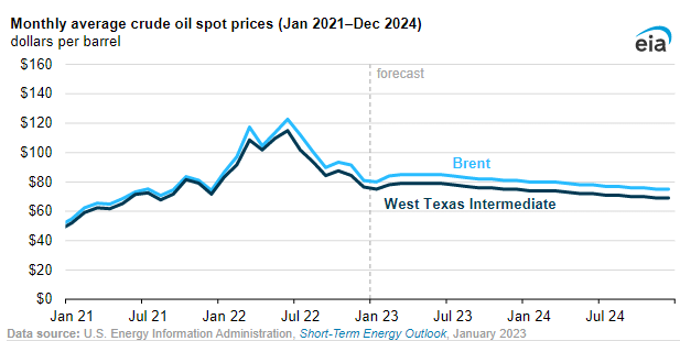
- The Paris-based EIA significantly lowered its price forecast for Brent crude oil for 2023 and 2024. The agency in its short term energy outlook lowered Brent price forecast to $83.1 per barrel for 2023 versus its previous forecast of $92.3 per barrel. This compares to the 2022 average price of $100.94 per barrel i.e. a decline of 18 per cent in 2023. The forecast for 2024 was further lower at $77.57, a y-o-y decline of 6.6 per cent. In terms of monthly trend, Brent crude averaged at $80.4 during December-2022 after witnessing a monthly decline of 11.8 per cent, the biggest decline since April-2020. The decline in Opec crude basket was similar at 11.2 per cent to average at $79.7 per barrel.
SeekingAlpha Long Ideas
- Crude oil prices have continued to decline in the last six months.
- Chevron’s high profitability will not stand in a market of lower crude oil prices.
- Management is making a big mistake repurchasing stock at top dollar prices.
TradingView Insights
WTI 1Y Chart:
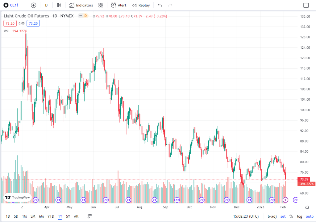
Technical analysis summary for Light Crude Oil Futures:

Brent 1Y Chart:

Short Ideas:

IEA Mid-Term Outlook
We forecast the Brent price will stay relatively flat through 2Q23, averaging $85/b, and then decline through the end of 2024. We expect the Brent price will average $83/b in 2023 and $78/b in 2024, down from $101/b in 2022. The West Texas Intermediate (WTI) price (the U.S. benchmark price) is forecast to generally follow a similar path, averaging $77/b in 2023 and $72/b 2024.
Principal contributor: Matthew French
Tags: production/supply, consumption/demand, spot prices, STEO (Short-Term Energy Outlook), Brent, crude oil, oil/petroleum, WTI (West Texas Intermediate)
SARIMAX WTI Forecast
Let’s set the working directory YOURPATH
import os
os.chdir(‘YOURPATH’)
os. getcwd()
and import the key libraries
import numpy as np
import pandas as pd
import yfinance as yf
from matplotlib import pyplot as plt
from statsmodels.tsa.stattools import adfuller
from statsmodels.tsa.seasonal import seasonal_decompose
from statsmodels.tsa.arima_model import ARIMA
from pandas.plotting import register_matplotlib_converters
register_matplotlib_converters()
Let’s read the input data
df = yf.download(‘CL=F’, ‘2022-02-03’)
[*********************100%***********************] 1 of 1 completed
and check the content as
df.tail()

Let’s drop the unwanted columns to focus on “Adj Close”
df=df.drop([‘Open’, ‘High’, ‘Low’, ‘Close’,’Volume’], axis=1)
df.tail()

and check the null values if any
df.isnull().sum()
Adj Close    0
dtype: int64
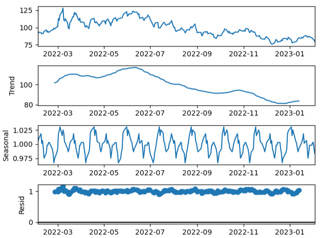
Let’s perform the ETS decomposition of this column with model=’additive’ and period=30 (1 month)
result = seasonal_decompose(df, model=’additive’,period=30)
result.plot()

Recall that ETS stands for Error-Trend-Seasonality and is a model used for the time series decomposition. It decomposes the series into the error, trend and seasonality component. It is a univariate forecasting model used when dealing with time-series data. It focuses on trend and seasonal components.
Let’s try ETS with model=’multiplicative’
result = seasonal_decompose(df, model=’multiplicative’,period=30)
result.plot()

Let’s check the ADF test
adfuller(df[‘Adj Close’])
(-0.9251431077004176,
 0.7795797169900887,
 6,
 247,
 {'1%': -3.457105309726321,
  '5%': -2.873313676101283,
  '10%': -2.5730443824681606},
 1205.1876481202412)
Recall that ADF (Augmented Dickey-Fuller) test is a statistical significance test which means the test will give results in hypothesis tests with null and alternative hypotheses. As a result, we will have a p-value from which we will need to make inferences about the time series, whether it is stationary or not.
Remark:
Following the TSA guide, we can verify our results using the TSA 1-day difference in the logarithmic scale
df[‘logarithm_base1’] = np.log2(df[‘Adj Close’])
data_d=df.diff(axis = 0, periods = 1)
Now let’s install pmarima
!pip install pmdarima
and import the library
from pmdarima import auto_arima
while ignoring harmless warnings
import warnings
warnings.filterwarnings(“ignore”)
Let’s fit auto_arima function to dataset
stepwise_fit = auto_arima(df[‘Adj Close’], start_p = 1, start_q = 1,
max_p = 3, max_q = 3, m = 12,
start_P = 0, seasonal = True,
d = None, D = 1, trace = True,
error_action =’ignore’,
suppress_warnings = True,
stepwise = True)
Let’s print the summary
stepwise_fit.summary()
stepwise_fit.summary()
Performing stepwise search to minimize aic
 ARIMA(1,0,1)(0,1,1)[12] intercept   : AIC=1265.376, Time=0.49 sec
 ARIMA(0,0,0)(0,1,0)[12] intercept   : AIC=1683.058, Time=0.01 sec
 ARIMA(1,0,0)(1,1,0)[12] intercept   : AIC=1322.398, Time=0.22 sec
 ARIMA(0,0,1)(0,1,1)[12] intercept   : AIC=1504.076, Time=0.25 sec
 ARIMA(0,0,0)(0,1,0)[12]             : AIC=1682.663, Time=0.05 sec
 ARIMA(1,0,1)(0,1,0)[12] intercept   : AIC=1370.656, Time=0.07 sec
 ARIMA(1,0,1)(1,1,1)[12] intercept   : AIC=inf, Time=0.69 sec
 ARIMA(1,0,1)(0,1,2)[12] intercept   : AIC=inf, Time=1.50 sec
 ARIMA(1,0,1)(1,1,0)[12] intercept   : AIC=1323.947, Time=0.26 sec
 ARIMA(1,0,1)(1,1,2)[12] intercept   : AIC=inf, Time=1.82 sec
 ARIMA(1,0,0)(0,1,1)[12] intercept   : AIC=1264.151, Time=0.27 sec
 ARIMA(1,0,0)(0,1,0)[12] intercept   : AIC=1368.690, Time=0.04 sec
 ARIMA(1,0,0)(1,1,1)[12] intercept   : AIC=inf, Time=0.52 sec
 ARIMA(1,0,0)(0,1,2)[12] intercept   : AIC=inf, Time=1.34 sec
 ARIMA(1,0,0)(1,1,2)[12] intercept   : AIC=inf, Time=1.53 sec
 ARIMA(0,0,0)(0,1,1)[12] intercept   : AIC=1684.885, Time=0.16 sec
 ARIMA(2,0,0)(0,1,1)[12] intercept   : AIC=1265.457, Time=0.43 sec
 ARIMA(2,0,1)(0,1,1)[12] intercept   : AIC=inf, Time=0.75 sec
 ARIMA(1,0,0)(0,1,1)[12]             : AIC=1264.289, Time=0.21 sec

Best model:  ARIMA(1,0,0)(0,1,1)[12] intercept
Total fit time: 10.635 seconds

Warnings: Covariance matrix calculated using the outer product of gradients (complex-step).
Let’s split our data into train / test sets
train = df.iloc[:len(df)-12]
test = df.iloc[len(df)-12:] # set one year(12 months) for testing
Let’s fit a SARIMAX(0, 1, 1)x(2, 1, 1, 12) on the training set:
from statsmodels.tsa.statespace.sarimax import SARIMAX
model = SARIMAX(train[‘Adj Close’],
order = (0, 1, 1),
seasonal_order =(2, 1, 1, 12))
result = model.fit()
result.summary()

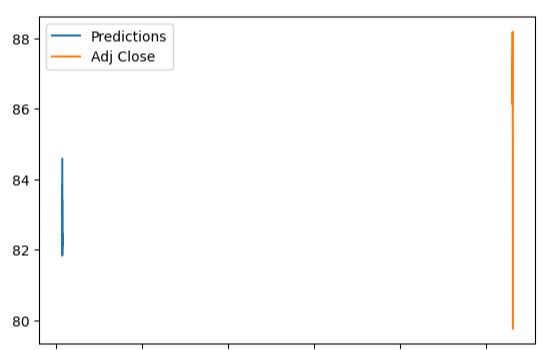
Let’s check 1Y predictions against the test set
start = len(train)
end = len(train) + len(test) – 1
predictions = result.predict(start, end,
typ = ‘levels’).rename(“Predictions”)
predictions.plot(legend = True)
test[‘Adj Close’].plot(legend = True)

Let’s check the 1Y start/end monthly time stamps
print (start,end)
242 253
The X-plot test[‘Adj Close’] vs predictions is

We have the following table
print(test[‘Adj Close’],predictions)
Date
2023-01-19    80.330002
2023-01-20    81.309998
2023-01-23    81.620003
2023-01-24    80.129997
2023-01-25    80.150002
2023-01-26    81.010002
2023-01-27    79.680000
2023-01-30    77.900002
2023-01-31    78.870003
2023-02-01    76.410004
2023-02-02    75.879997
2023-02-03    73.230003
Name: Adj Close, dtype: float64 242    78.798398
243    78.018756
244    79.072597
245    78.460463
246    78.198427
247    78.346828
248    77.993672
249    77.691316
250    77.831578
251    78.591275
252    78.351060
253    77.758151
Name: Predictions, dtype: float64
In principle, we can obtain m (slope) and b(intercept) of a linear regression line
x=test[‘Adj Close’]
y=predictions
plt.plot(x,y, ‘o’, color=’green’)
m, b = np.polyfit(x, y, 1)
and use red as color for our linear regression line
plt.plot(x, m*x+b, color=’red’)

Let’s load the 2 evaluation metrics
from sklearn.metrics import mean_squared_error
from statsmodels.tools.eval_measures import rmse
to calculate the root mean squared (RMS) error
rmse(test[“Adj Close”], predictions)
2.3925166812892513
and the mean squared error (MSE)
mean_squared_error(test[“Adj Close”], predictions)
5.724136070247333
Let’s train the model on the full dataset
model = model = SARIMAX(df[‘Adj Close’],
order = (0, 1, 1),
seasonal_order =(2, 1, 1, 12))
result = model.fit()
forecast = result.predict(start = len(df),
end = (len(df)-1) + 1 * 12,
typ = ‘levels’).rename(‘Forecast’)
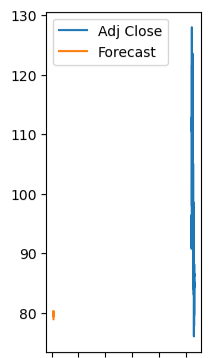
f[‘Adj Close’].plot(figsize = (2, 5), legend = True)
forecast.plot(legend = True)

Let’s print 1Y forecast
print(forecast)
54    73.326667
255    73.101625
256    73.790496
257    73.141656
258    72.914942
259    73.351366
260    72.530161
261    72.079887
262    72.225980
263    72.528791
264    71.986863
265    71.282966
and plot it
plt.plot(forecast)
plt.xlabel(“254+(Month Number 0-11)”);
plt.ylabel(“Predicted Oil Price $”);

Recall that
len(forecast)
12
This prediction is within the IEA forecast range 70 < WTI price < Brent price < 80 USD in 2023. Recall the IEA forecast: the average WTI price (the U.S. benchmark price) is ca. $77/b in 2023.
The above plot suggests that WTI price ~ 73 +/- 6 USD.
Indeed our forecast error is ca. 6 USD.
SARIMAX Brent Forecast
Let’s look at the Brent Crude Oil (BZ=F)
f = yf.download(‘BZ=F’, ‘2022-02-03’)
[*********************100%***********************] 1 of 1 completed
df.tail()

The target variable is
df=df.drop([‘Open’, ‘High’, ‘Low’, ‘Close’,’Volume’], axis=1)
df.tail()

with no null values
df.isnull().sum()
Adj Close    0
dtype: int64
The ETS Decomposition is
result = seasonal_decompose(df, model=’additive’,period=30)
result.plot()

result = seasonal_decompose(df, model=’multiplicative’,period=30)
result.plot()
The ADF test is
adfuller(df[‘Adj Close’])
(-0.8024986505767407,
 0.8183870058478762,
 10,
 243,
 {'1%': -3.4575505077947746,
  '5%': -2.8735087323013526,
  '10%': -2.573148434859185},
 1216.2416870507893)
Let’s fit auto_arima function to our dataset
stepwise_fit = auto_arima(df[‘Adj Close’], start_p = 1, start_q = 1,
max_p = 3, max_q = 3, m = 12,
start_P = 0, seasonal = True,
d = None, D = 1, trace = True,
error_action =’ignore’,
suppress_warnings = True,
stepwise = True)
stepwise_fit.summary()
Performing stepwise search to minimize aic
 ARIMA(1,1,1)(0,1,1)[12]             : AIC=inf, Time=0.67 sec
 ARIMA(0,1,0)(0,1,0)[12]             : AIC=1399.118, Time=0.01 sec
 ARIMA(1,1,0)(1,1,0)[12]             : AIC=1346.586, Time=0.08 sec
 ARIMA(0,1,1)(0,1,1)[12]             : AIC=inf, Time=0.71 sec
 ARIMA(1,1,0)(0,1,0)[12]             : AIC=1399.664, Time=0.02 sec
 ARIMA(1,1,0)(2,1,0)[12]             : AIC=1313.799, Time=0.22 sec
 ARIMA(1,1,0)(2,1,1)[12]             : AIC=inf, Time=1.75 sec
 ARIMA(1,1,0)(1,1,1)[12]             : AIC=inf, Time=0.63 sec
 ARIMA(0,1,0)(2,1,0)[12]             : AIC=1311.810, Time=0.14 sec
 ARIMA(0,1,0)(1,1,0)[12]             : AIC=1344.608, Time=0.05 sec
 ARIMA(0,1,0)(2,1,1)[12]             : AIC=inf, Time=1.53 sec
 ARIMA(0,1,0)(1,1,1)[12]             : AIC=inf, Time=0.52 sec
 ARIMA(0,1,1)(2,1,0)[12]             : AIC=1313.799, Time=0.22 sec
 ARIMA(1,1,1)(2,1,0)[12]             : AIC=1315.738, Time=0.46 sec
 ARIMA(0,1,0)(2,1,0)[12] intercept   : AIC=1313.689, Time=0.58 sec

Best model:  ARIMA(0,1,0)(2,1,0)[12]
Total fit time: 7.603 seconds

Let’s split our data into the train / test sets
train = df.iloc[:len(df)-12]
test = df.iloc[len(df)-12:] # set one year(12 months) for testing
Fit the best SARIMAX model to the training set
model = SARIMAX(train[‘Adj Close’],
order = (0, 1, 0),
seasonal_order =(2, 1, 0, 12))
result = model.fit()
result.summary()

Let’s make our predictions for one-year against the test set
start = len(train)
end = len(train) + len(test) – 1
predictions = result.predict(start, end,
typ = ‘levels’).rename(“Predictions”)
predictions.plot(legend = True)
test[‘Adj Close’].plot(legend = True)
let’s check the time/month stamp
print (start,end)
242 253
The X-plot predicted vs observed prices test data is
plt.scatter(test[‘Adj Close’],predictions)
plt.xlabel(‘Adj Close Test’)
plt.ylabel(‘Predictions’)

The corresponding table is
print(test[‘Adj Close’],predictions)
Date
2023-01-19    86.160004
2023-01-20    87.629997
2023-01-23    88.190002
2023-01-24    86.129997
2023-01-25    86.120003
2023-01-26    87.470001
2023-01-27    86.660004
2023-01-30    84.900002
2023-01-31    84.489998
2023-02-01    82.839996
2023-02-02    82.169998
2023-02-03    79.760002
Name: Adj Close, dtype: float64 242    84.737661
243    83.124420
244    84.063293
245    83.656751
246    83.973558
247    84.280618
248    84.402494
249    84.300495
250    84.832498
251    85.114817
252    84.739011
253    84.193353
Name: Predictions, dtype: float64
we can obtain m (slope) and b(intercept) of a linear regression line
x=test[‘Adj Close’]
y=predictions
plt.plot(x,y, ‘o’, color=’green’)
m, b = np.polyfit(x, y, 1)
using red as a color for our linear regression line
plt.plot(x, m*x+b, color=’red’)
plt.xlabel(‘Adj Close Test’)
plt.ylabel(‘Predictions’)

Let’s calculate the RMSE
rmse(test[“Adj Close”], predictions)
3.672425747417604
and the corresponding MSE
mean_squared_error(test[“Adj Close”], predictions)
13.486710870295747
Let’s train the model on the full dataset
model = model = SARIMAX(df[‘Adj Close’],
order = (0, 1, 1),
seasonal_order =(2, 1, 1, 12))
result = model.fit()
forecast = result.predict(start = len(df),
end = (len(df)-1) + 1 * 12,
typ = ‘levels’).rename(‘Forecast’)
df[‘Adj Close’].plot(figsize = (2, 5), legend = True)
forecast.plot(legend = True)
We can print the table
print(forecast)
254    80.319296
255    79.393284
256    80.083311
257    79.554758
258    79.718730
259    80.245928
260    79.837283
261    79.581158
262    79.910810
263    80.090715
264    79.351650
265    78.977657
Name: Forecast, dtype: float64
and plot the corresponding 1Y forecast
plt.plot(forecast)
plt.xlabel(“254+(Month Number 0-11)”);
plt.ylabel(“Predicted Brent Oil Price $”);

Recall that IEA expect the Brent price will average $83/b in 2023. This plot suggests that the average Brent price would be 80 +/-13 USD.
Summary
- We have downgraded the EIA’s 2023 WTI/Brent oil price forecast. This appears to be consistent with the JPMorgan adjustment of its forecast. However, a fully effective transatlantic embargo would pull a considerable amount of oil from the market, leading to higher oil prices.
- Due to vulnerability to geopolitical developments, the oil market is characterized by significant uncertainties in 2023 and beyond. It turns out that relatively large error bars of our SARIMAX predicted oil price values support the expected volatility of the energy market in a single graph.
- A U.S. recession in 2023 could spark a new crude oil bear market, posing a significant challenge to Big Oil earnings and cash flow growth.
- Generally, as the economy transitions from peak productivity, high inflation, and labor shortages to a recession-like environment with softer economic activity, lower employment numbers, and potentially evaporating demand for crude oil and other energy sources, the market must expect an ongoing decline in profitability.
Bottom Line: Crude Oil Prices Are Set For Mean Reversion.
Explore More
(S)ARIMA(X) TSA Forecasting, QC and Visualization of E-Commerce Food Delivery Sales
Stock Market ’22 Round Up & ’23 Outlook: Zacks Strategy vs Seeking Alpha Tactics
XOM SMA-EMA-RSI Golden Crosses ’22
Energy E&P: XOM Technical Analysis Nov ’22
The Zacks Market Outlook Nov ’22 – Energy
OXY Stock Technical Analysis 17 May 2022
Embed Socials


Make a one-time donation
Make a monthly donation
Make a yearly donation
Choose an amount
Or enter a custom amount
Your contribution is appreciated.
Your contribution is appreciated.
Your contribution is appreciated.
DonateDonate monthlyDonate yearly
Leave a comment