
- Machine Learning (ML) and Deep Learning (DL) play a crucial role in managing efficient supply chain operations in the fashion retail industry.
- Apart from large e-commerce brands like Amazon, even small-time fashion retailers are now using ML algorithms to understand fast-changing customer needs and expectations.
- Neural network (NN) models are considered the most efficient and accurate forecasting methods, as they have demonstrated high performance in various business applications involving fashion e-commerce digital platforms.
- The goal of the present DL project is to train and optimize a Tensor Flow (TF) / Keras Convolution Neural Network (CNN), enabling us to classify the MNIST fashion clothing images.
- In fact, fashion clothing DL is the familiar problem of multi-label image classification. The key benefit of CNN is that the number of training model parameters is independent of the size of the original image.
- Following earlier DL studies, we train a Feedforward CNN model to classify images of clothing on train data and make predictions on test data. We use tf.keras throughout the project, a high-level API to build and train models in TensorFlow.
The Fashion MNIST Dataset
Fashion-MNIST is a dataset of Zalando’s article images—consisting of a training set of 60,000 examples and a test set of 10,000 examples. Each example is a 28×28 grayscale image, associated with a label from 10 classes:
- 0 T-shirt/top
- 1 Trouser
- 2 Pullover
- 3 Dress
- 4 Coat
- 5 Sandal
- 6 Shirt
- 7 Sneaker
- 8 Bag
- 9 Ankle boot
Each image pixel has a single pixel-value associated with it, indicating the lightness or darkness of that pixel, with higher numbers meaning darker. This pixel-value is an integer between 0 and 255.
We aim to feed a 28 x 28 image (784 bytes) as an input to CNN, so that CNN can classify the image as one of the item labels.
Model Version 1
Let’s set the working directory YOURPATH
import os
os.chdir(‘YOURPATH’)
os. getcwd()
and import the following key libraries
import tensorflow as tf
import numpy as np
import matplotlib.pyplot as plt
print(tf.version)
2.10.0
Let’s load the input data
fashion_mnist = tf.keras.datasets.fashion_mnist
(train_images, train_labels), (test_images, test_labels) = fashion_mnist.load_data()
and check the data structure
train_images.shape
(60000, 28, 28)
len(train_labels)
60000
test_images.shape
(10000, 28, 28)
len(test_labels)
10000
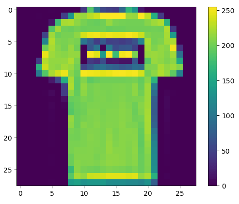
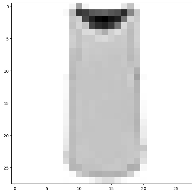
Let’s plot a single image
plt.figure()
plt.imshow(train_images[1])
plt.colorbar()
plt.grid(False)
plt.show()
Let’s scale the images
train_images = train_images / 255.0
test_images = test_images / 255.0
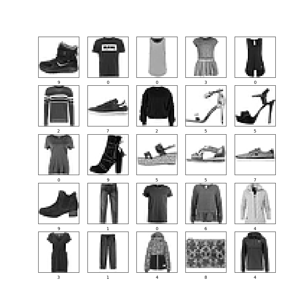
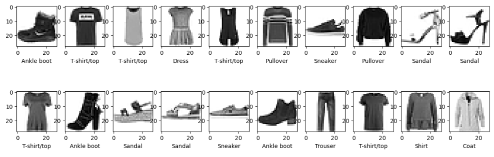
and plot 25 selected grayscale labeled images
plt.figure(figsize=(10,10))
for i in range(25):
plt.subplot(5,5,i+1)
plt.xticks([])
plt.yticks([])
plt.grid(False)
plt.imshow(train_images[i], cmap=plt.cm.binary)
plt.xlabel(train_labels[i])
plt.savefig(‘example25grayscaleimages.png’)
Let’s design a simple CNN model, compile and train the model with optimizer=’adam’ and epochs=20
model = tf.keras.Sequential([
tf.keras.layers.Flatten(input_shape=(28, 28)),
tf.keras.layers.Dense(128, activation=’relu’),
tf.keras.layers.Dense(10)])
model.compile(optimizer=’adam’,
loss=tf.keras.losses.SparseCategoricalCrossentropy(from_logits=True),
metrics=[‘accuracy’])
model.fit(train_images, train_labels, epochs=20)
Epoch 1/20
1875/1875 [==============================] - 3s 2ms/step - loss: 0.5018 - accuracy: 0.8240
Epoch 2/20
1875/1875 [==============================] - 3s 2ms/step - loss: 0.3791 - accuracy: 0.8625
Epoch 3/20
1875/1875 [==============================] - 3s 2ms/step - loss: 0.3360 - accuracy: 0.8773
Epoch 4/20
1875/1875 [==============================] - 3s 2ms/step - loss: 0.3139 - accuracy: 0.8862
Epoch 5/20
1875/1875 [==============================] - 3s 2ms/step - loss: 0.2936 - accuracy: 0.8909
Epoch 6/20
1875/1875 [==============================] - 3s 2ms/step - loss: 0.2817 - accuracy: 0.8954
Epoch 7/20
1875/1875 [==============================] - 3s 2ms/step - loss: 0.2692 - accuracy: 0.8990
Epoch 8/20
1875/1875 [==============================] - 3s 2ms/step - loss: 0.2573 - accuracy: 0.9045
Epoch 9/20
1875/1875 [==============================] - 3s 2ms/step - loss: 0.2480 - accuracy: 0.9074
Epoch 10/20
1875/1875 [==============================] - 3s 2ms/step - loss: 0.2390 - accuracy: 0.9099
Epoch 11/20
1875/1875 [==============================] - 3s 2ms/step - loss: 0.2316 - accuracy: 0.9134
Epoch 12/20
1875/1875 [==============================] - 3s 2ms/step - loss: 0.2233 - accuracy: 0.9159
Epoch 13/20
1875/1875 [==============================] - 3s 2ms/step - loss: 0.2168 - accuracy: 0.9195
Epoch 14/20
1875/1875 [==============================] - 3s 2ms/step - loss: 0.2121 - accuracy: 0.9212
Epoch 15/20
1875/1875 [==============================] - 3s 2ms/step - loss: 0.2066 - accuracy: 0.9217
Epoch 16/20
1875/1875 [==============================] - 3s 2ms/step - loss: 0.2005 - accuracy: 0.9251
Epoch 17/20
1875/1875 [==============================] - 3s 2ms/step - loss: 0.1939 - accuracy: 0.9267
Epoch 18/20
1875/1875 [==============================] - 3s 2ms/step - loss: 0.1913 - accuracy: 0.9278
Epoch 19/20
1875/1875 [==============================] - 3s 2ms/step - loss: 0.1848 - accuracy: 0.9305
Epoch 20/20
1875/1875 [==============================] - 3s 2ms/step - loss: 0.1806 - accuracy: 0.9312
Let’s check the CNN loss/accuracy
test_loss, test_acc = model.evaluate(test_images, test_labels, verbose=2)
print(‘\nTest accuracy:’, test_acc)
313/313 - 0s - loss: 0.3805 - accuracy: 0.8783 - 441ms/epoch - 1ms/step

Test accuracy: 0.8783000111579895
Let’s make predictions using test images
probability_model = tf.keras.Sequential([model,
tf.keras.layers.Softmax()])
predictions = probability_model.predict(test_images)
313/313 [==============================] - 0s 645us/step
predictions[1]
array([4.9210530e-06, 3.8770574e-15, 9.9937904e-01, 3.7104611e-11,
       5.7768257e-04, 1.3045125e-12, 3.8408274e-05, 1.2573967e-21,
       8.8773615e-12, 2.4979118e-16], dtype=float32)
We can see that
np.argmax(predictions[1])
2
which is consistent with the true test label
test_labels[1]
2
Let’s invoke a couple of image plot functions
def plot_image(i, predictions_array, true_label, img):
true_label, img = true_label[i], img[i]
plt.grid(False)
plt.xticks([])
plt.yticks([])
plt.imshow(img, cmap=plt.cm.binary)
predicted_label = np.argmax(predictions_array)
if predicted_label == true_label:
color = ‘blue’
else:
color = ‘red’
plt.xlabel(“{} {:2.0f}% ({})”.format(predicted_label,
100*np.max(predictions_array),
true_label),
color=color)
def plot_value_array(i, predictions_array, true_label):
true_label = true_label[i]
plt.grid(False)
plt.xticks(range(10))
plt.yticks([])
thisplot = plt.bar(range(10), predictions_array, color=”#777777″)
plt.ylim([0, 1])
predicted_label = np.argmax(predictions_array)
thisplot[predicted_label].set_color(‘red’)
thisplot[true_label].set_color(‘blue’)
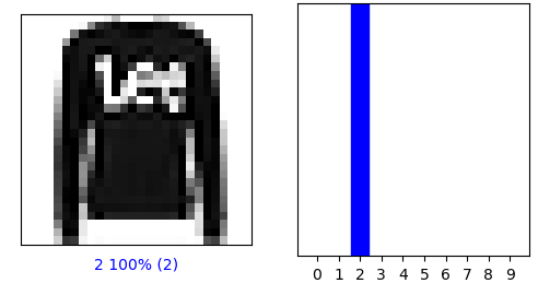
Let’s plot a couple of selected images
i = 1
plt.figure(figsize=(6,3))
plt.subplot(1,2,1)
plot_image(i, predictions[i], test_labels, test_images)
plt.subplot(1,2,2)
plot_value_array(i, predictions[i], test_labels)
plt.show()
true label =2
i = 12
plt.figure(figsize=(6,3))
plt.subplot(1,2,1)
plot_image(i, predictions[i], test_labels, test_images)
plt.subplot(1,2,2)
plot_value_array(i, predictions[i], test_labels)
plt.show()
true label =7

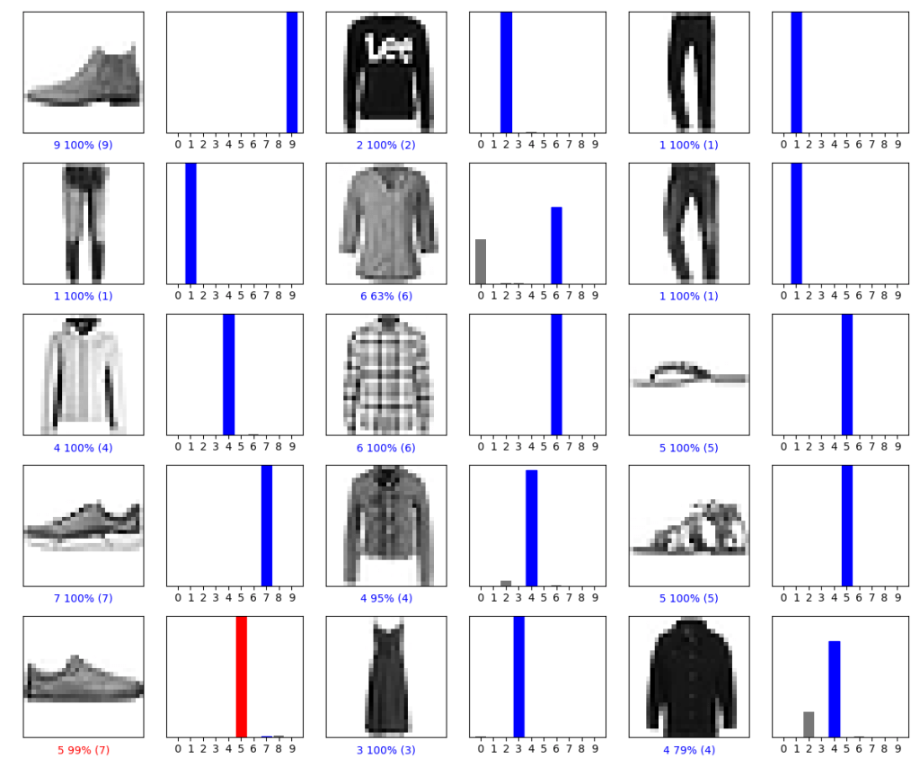
Let’s plot several test images, their predicted labels, and the true labels (recall that we color correct predictions in blue and incorrect predictions in red)
num_rows = 5
num_cols = 3
num_images = num_rowsnum_cols plt.figure(figsize=(22num_cols, 2num_rows))
for i in range(num_images):
plt.subplot(num_rows, 2num_cols, 2i+1)
plot_image(i, predictions[i], test_labels, test_images)
plt.subplot(num_rows, 2num_cols, 2i+2)
plot_value_array(i, predictions[i], test_labels)
plt.tight_layout()
plt.savefig(‘clothestrainpredict.png’)
We can grab an image from the test dataset
img = test_images[1]
print(img.shape)
Add the image to a batch where it’s the only member
img = (np.expand_dims(img,0))
print(img.shape)
predictions_single = probability_model.predict(img)
print(predictions_single)
(28, 28)
(1, 28, 28)
1/1 [==============================] - 0s 16ms/step
[[4.9210530e-06 3.8770574e-15 9.9937904e-01 3.7104611e-11 5.7768257e-04
  1.3045125e-12 3.8408274e-05 1.2573967e-21 8.8773615e-12 2.4979118e-16]]
plot_value_array(1, predictions_single[0], test_labels)
plt.show()
![Probability of label=2 for test_images[1]](https://newdigitals.org/wp-content/uploads/2023/01/plotimage2.png?w=522)
Model Version 2
Recall that we need to import the key libraries and prepare the input data
import tensorflow as tf
import numpy as np
import matplotlib.pyplot as plt
clothing_fashion_mnist = tf.keras.datasets.fashion_mnist
while loading the dataset from tensorflow
(x_train, y_train),(x_test, y_test) = clothing_fashion_mnist.load_data()
and displaying the shapes of training and testing datasets
print(‘Shape of training cloth images: ‘,
x_train.shape)
print(‘Shape of training label: ‘,
y_train.shape)
print(‘Shape of test cloth images: ‘,
x_test.shape)
print(‘Shape of test labels: ‘,
y_test.shape)
Shape of training cloth images:  (60000, 28, 28)
Shape of training label:  (60000,)
Shape of test cloth images:  (10000, 28, 28)
Shape of test labels:  (10000,)
Let’s store the class names
label_class_names = [‘T-shirt/top’, ‘Trouser’,
‘Pullover’, ‘Dress’, ‘Coat’,
‘Sandal’, ‘Shirt’, ‘Sneaker’,
‘Bag’, ‘Ankle boot’]
and display the selected image ii=2 with the colorbar
plt.imshow(x_train[ii])
plt.colorbar()
plt.show()

Let’s normalize both training and testing datasets
x_train = x_train / 255.0
x_test = x_test / 255.0
let’s plot the first 20 training images
plt.figure(figsize=(15, 5)) # figure size
i = 0
while i < 20:
plt.subplot(2, 10, i+1)
plt.imshow(x_train[i], cmap=plt.cm.binary)
plt.xlabel(label_class_names[y_train[i]])
i = i+1
plt.show()
Let’s build the model
model = tf.keras.Sequential([
tf.keras.layers.Flatten(input_shape=(28, 28)),
tf.keras.layers.Dense(128, activation=’relu’),
tf.keras.layers.Dense(10)
])
compile the model
model.compile(optimizer=’adam’,
loss=tf.keras.losses.SparseCategoricalCrossentropy(
from_logits=True),
metrics=[‘accuracy’])
and fit the model to the training data
model.fit(x_train, y_train, epochs=20)
Epoch 1/20
1875/1875 [==============================] - 10s 5ms/step - loss: 0.4958 - accuracy: 0.8256
Epoch 2/20
1875/1875 [==============================] - 9s 5ms/step - loss: 0.3726 - accuracy: 0.8647
Epoch 3/20
1875/1875 [==============================] - 9s 5ms/step - loss: 0.3324 - accuracy: 0.8790
Epoch 4/20
1875/1875 [==============================] - 9s 5ms/step - loss: 0.3115 - accuracy: 0.8865
Epoch 5/20
1875/1875 [==============================] - 9s 5ms/step - loss: 0.2932 - accuracy: 0.8913
Epoch 6/20
1875/1875 [==============================] - 9s 5ms/step - loss: 0.2772 - accuracy: 0.8974
Epoch 7/20
1875/1875 [==============================] - 9s 5ms/step - loss: 0.2662 - accuracy: 0.9006
Epoch 8/20
1875/1875 [==============================] - 9s 5ms/step - loss: 0.2559 - accuracy: 0.9043
Epoch 9/20
1875/1875 [==============================] - 9s 5ms/step - loss: 0.2471 - accuracy: 0.9082
Epoch 10/20
1875/1875 [==============================] - 9s 5ms/step - loss: 0.2377 - accuracy: 0.9115
Epoch 11/20
1875/1875 [==============================] - 9s 5ms/step - loss: 0.2305 - accuracy: 0.9125
Epoch 12/20
1875/1875 [==============================] - 9s 5ms/step - loss: 0.2236 - accuracy: 0.9163
Epoch 13/20
1875/1875 [==============================] - 9s 5ms/step - loss: 0.2156 - accuracy: 0.9190
Epoch 14/20
1875/1875 [==============================] - 9s 5ms/step - loss: 0.2106 - accuracy: 0.9215
Epoch 15/20
1875/1875 [==============================] - 9s 5ms/step - loss: 0.2064 - accuracy: 0.9224
Epoch 16/20
1875/1875 [==============================] - 9s 5ms/step - loss: 0.1977 - accuracy: 0.9251
Epoch 17/20
1875/1875 [==============================] - 9s 5ms/step - loss: 0.1925 - accuracy: 0.9283
Epoch 18/20
1875/1875 [==============================] - 9s 5ms/step - loss: 0.1882 - accuracy: 0.9295
Epoch 19/20
1875/1875 [==============================] - 9s 5ms/step - loss: 0.1845 - accuracy: 0.9306
Epoch 20/20
1875/1875 [==============================] - 9s 5ms/step - loss: 0.1796 - accuracy: 0.9328
Let’s calculate loss/accuracy score
test_loss, test_acc = model.evaluate(x_test,
y_test,
verbose=2)
print(‘\nTest loss:’, test_loss)
print(‘\nTest accuracy:’, test_acc)
313/313 - 1s - loss: 0.3656 - accuracy: 0.8845 - 1s/epoch - 4ms/step

Test loss: 0.3656046390533447

Test accuracy: 0.8845000267028809
We use Softmax() function to convert linear output logits to probability
prediction_model = tf.keras.Sequential(
[model, tf.keras.layers.Softmax()])
and make predictions of test data
prediction = prediction_model.predict(x_test)
Let’s look at the test image with ii=1
print(‘Predicted test label:’, np.argmax(prediction[ii]))
print(label_class_names[np.argmax(prediction[ii])])
print(‘Actual test label:’, y_test[ii])
313/313 [==============================] - 0s 1ms/step
Predicted test label: 1
Trouser
Actual test label: 1
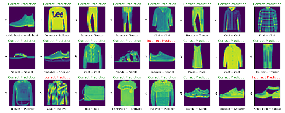
Let’s plot 24 selected test images
plt.figure(figsize=(15, 6))
i = 0
while i < 24:
image, actual_label = x_test[i], y_test[i]
predicted_label = np.argmax(prediction[i])
plt.subplot(3, 8, i+1)
plt.tight_layout()
plt.xticks([])
plt.yticks([])
# display plot
plt.imshow(image)

# if else condition to distinguish right and
# wrong
if predicted_label == actual_label:color, label = ('green', 'Correct Prediction')
if predicted_label != actual_label:color, label = ('red', 'Incorrect Prediction')

# plotting labels and giving color to it
# according to its correctness
plt.title(label, color=color)

# labelling the images in x-axis to see
# the correct and incorrect results
plt.xlabel(" {} ~ {} ".format(
    label_class_names[actual_label],
  label_class_names[predicted_label]))

# labelling the images orderwise in y-axis
plt.ylabel(i)
# incrementing counter variable
i += 1
Model Version 3
Let’s import the key libraries and load the input dataset
import numpy as np
import pandas as pd
import matplotlib.pyplot as plt
import seaborn as sns
import keras
import tensorflow as tf
print(tf.version)
2.10.0
fashion_mnist = tf.keras.datasets.fashion_mnist
(X_train, y_train), (X_test, y_test) = fashion_mnist.load_data()
Let’s explore the dataset
Check the shape and size of X_train, X_test, y_train, y_test
print (“Number of observations in training data: ” + str(len(X_train)))
print (“Number of labels in training data: ” + str(len(y_train)))
print (“Dimensions of a single image in X_train:” + str(X_train[0].shape))
print(“————————————————————-\n”)
print (“Number of observations in test data: ” + str(len(X_test)))
print (“Number of labels in test data: ” + str(len(y_test)))
print (“Dimensions of single image in X_test:” + str(X_test[0].shape))
Number of observations in training data: 60000
Number of labels in training data: 60000
Dimensions of a single image in X_train:(28, 28)
-------------------------------------------------------------

Number of observations in test data: 10000
Number of labels in test data: 10000
Dimensions of single image in X_test:(28, 28)
Let’s set the label list
class_labels = [‘T-shirt/top’,’Trouser’,’Pullover’,’Dress’,’Coat’,’Sandal’,’Shirt’,’Sneakers’,’Bag’,’Ankle boot’]
and plot the selected training image
ii=1
plt.figure(figsize = (8,8))
plt.imshow(X_train[ii],cmap = ‘Greys’);
We can also plot the next image
ii1=ii+1
plt.figure(figsize = (8,8))
plt.imshow(X_train[ii1],cmap = ‘Greys’);
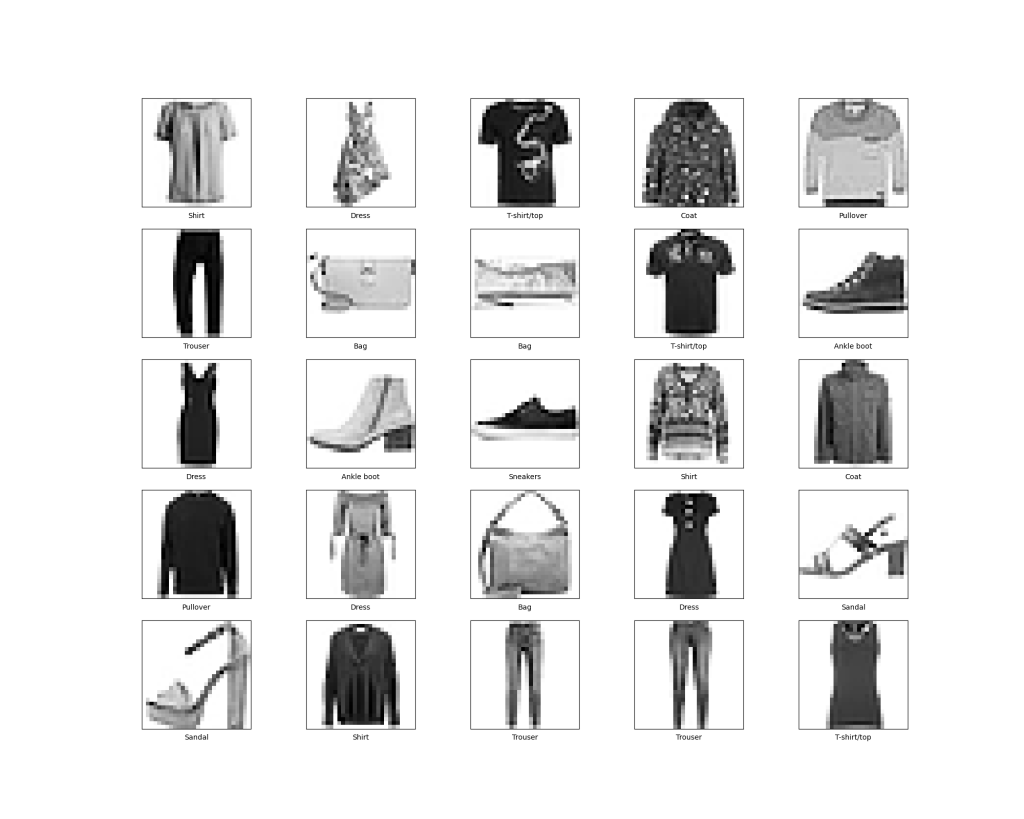
Let’s plot first 25 images from the training set and display the class name below each image
plt.figure(figsize=(20,16))
for i in range(25):
plt.subplot(5,5,i+1)
plt.xticks([])
plt.yticks([])
plt.grid(False)
plt.imshow(X_train[i], cmap=’Greys’)
plt.xlabel(class_labels[y_train[i]])
plt.savefig(‘clothesgrey.png’)
Let’s scale the data
X_train = X_train / 255.0
X_test = X_test / 255.0
and check the shape
X_train.shape , y_train.shape
((60000, 28, 28), (60000,))
Let’s build, compile and train the CNN model
model = tf.keras.Sequential([
tf.keras.layers.Flatten(input_shape=(28, 28)),
tf.keras.layers.Dense(128, activation=’relu’),
tf.keras.layers.Dense(10)])
model.compile(optimizer=’adam’,loss=tf.keras.losses.SparseCategoricalCrossentropy(from_logits=True),metrics=[‘accuracy’])
model.fit(X_train, y_train, epochs=50)
Epoch 1/50
1875/1875 [==============================] - 4s 2ms/step - loss: 0.4999 - accuracy: 0.8251
Epoch 2/50
1875/1875 [==============================] - 3s 2ms/step - loss: 0.3732 - accuracy: 0.8652
Epoch 3/50
1875/1875 [==============================] - 3s 2ms/step - loss: 0.3342 - accuracy: 0.8793
Epoch 4/50
1875/1875 [==============================] - 3s 2ms/step - loss: 0.3111 - accuracy: 0.8856
Epoch 5/50
1875/1875 [==============================] - 3s 2ms/step - loss: 0.2923 - accuracy: 0.8928
Epoch 6/50
1875/1875 [==============================] - 3s 2ms/step - loss: 0.2795 - accuracy: 0.8971
Epoch 7/50
1875/1875 [==============================] - 3s 2ms/step - loss: 0.2678 - accuracy: 0.9009
Epoch 8/50
1875/1875 [==============================] - 3s 2ms/step - loss: 0.2548 - accuracy: 0.9048
Epoch 9/50
1875/1875 [==============================] - 3s 2ms/step - loss: 0.2473 - accuracy: 0.9081
Epoch 10/50
1875/1875 [==============================] - 3s 2ms/step - loss: 0.2379 - accuracy: 0.9113
Epoch 11/50
1875/1875 [==============================] - 3s 2ms/step - loss: 0.2308 - accuracy: 0.9126
Epoch 12/50
1875/1875 [==============================] - 3s 2ms/step - loss: 0.2228 - accuracy: 0.9168
Epoch 13/50
1875/1875 [==============================] - 3s 2ms/step - loss: 0.2160 - accuracy: 0.9185
Epoch 14/50
1875/1875 [==============================] - 3s 2ms/step - loss: 0.2119 - accuracy: 0.9211
Epoch 15/50
1875/1875 [==============================] - 3s 2ms/step - loss: 0.2039 - accuracy: 0.9234
Epoch 16/50
1875/1875 [==============================] - 4s 2ms/step - loss: 0.1991 - accuracy: 0.9255
Epoch 17/50
1875/1875 [==============================] - 4s 2ms/step - loss: 0.1923 - accuracy: 0.9282
Epoch 18/50
1875/1875 [==============================] - 4s 2ms/step - loss: 0.1877 - accuracy: 0.9291
Epoch 19/50
1875/1875 [==============================] - 3s 2ms/step - loss: 0.1838 - accuracy: 0.9329
Epoch 20/50
1875/1875 [==============================] - 4s 2ms/step - loss: 0.1769 - accuracy: 0.9342
Epoch 21/50
1875/1875 [==============================] - 3s 2ms/step - loss: 0.1728 - accuracy: 0.9363
Epoch 22/50
1875/1875 [==============================] - 3s 2ms/step - loss: 0.1679 - accuracy: 0.9374
Epoch 23/50
1875/1875 [==============================] - 3s 2ms/step - loss: 0.1655 - accuracy: 0.9376
Epoch 24/50
1875/1875 [==============================] - 4s 2ms/step - loss: 0.1610 - accuracy: 0.9391
Epoch 25/50
1875/1875 [==============================] - 4s 2ms/step - loss: 0.1565 - accuracy: 0.9419
Epoch 26/50
1875/1875 [==============================] - 4s 2ms/step - loss: 0.1525 - accuracy: 0.9433
Epoch 27/50
1875/1875 [==============================] - 4s 2ms/step - loss: 0.1505 - accuracy: 0.9438
Epoch 28/50
1875/1875 [==============================] - 4s 2ms/step - loss: 0.1474 - accuracy: 0.9446
Epoch 29/50
1875/1875 [==============================] - 4s 2ms/step - loss: 0.1431 - accuracy: 0.9470
Epoch 30/50
1875/1875 [==============================] - 4s 2ms/step - loss: 0.1410 - accuracy: 0.9473
Epoch 31/50
1875/1875 [==============================] - 3s 2ms/step - loss: 0.1400 - accuracy: 0.9470
Epoch 32/50
1875/1875 [==============================] - 3s 2ms/step - loss: 0.1358 - accuracy: 0.9491
Epoch 33/50
1875/1875 [==============================] - 3s 2ms/step - loss: 0.1302 - accuracy: 0.9518
Epoch 34/50
1875/1875 [==============================] - 4s 2ms/step - loss: 0.1301 - accuracy: 0.9515
Epoch 35/50
1875/1875 [==============================] - 3s 2ms/step - loss: 0.1275 - accuracy: 0.9522
Epoch 36/50
1875/1875 [==============================] - 3s 2ms/step - loss: 0.1234 - accuracy: 0.9542
Epoch 37/50
1875/1875 [==============================] - 3s 2ms/step - loss: 0.1218 - accuracy: 0.9545
Epoch 38/50
1875/1875 [==============================] - 4s 2ms/step - loss: 0.1195 - accuracy: 0.9559
Epoch 39/50
1875/1875 [==============================] - 3s 2ms/step - loss: 0.1188 - accuracy: 0.9557
Epoch 40/50
1875/1875 [==============================] - 3s 2ms/step - loss: 0.1161 - accuracy: 0.9559
Epoch 41/50
1875/1875 [==============================] - 3s 2ms/step - loss: 0.1122 - accuracy: 0.9578
Epoch 42/50
1875/1875 [==============================] - 3s 2ms/step - loss: 0.1120 - accuracy: 0.9578
Epoch 43/50
1875/1875 [==============================] - 4s 2ms/step - loss: 0.1081 - accuracy: 0.9591
Epoch 44/50
1875/1875 [==============================] - 3s 2ms/step - loss: 0.1102 - accuracy: 0.9593
Epoch 45/50
1875/1875 [==============================] - 3s 2ms/step - loss: 0.1053 - accuracy: 0.9612
Epoch 46/50
1875/1875 [==============================] - 3s 2ms/step - loss: 0.1030 - accuracy: 0.9620
Epoch 47/50
1875/1875 [==============================] - 3s 2ms/step - loss: 0.1017 - accuracy: 0.9622
Epoch 48/50
1875/1875 [==============================] - 4s 2ms/step - loss: 0.1012 - accuracy: 0.9627
Epoch 49/50
1875/1875 [==============================] - 3s 2ms/step - loss: 0.0988 - accuracy: 0.9635
Epoch 50/50
1875/1875 [==============================] - 3s 2ms/step - loss: 0.0978 - accuracy: 0.9639
Model Accuracy Results:
print(“Results:”)
print(“———————“)
scores_train = model.evaluate(X_train, y_train, verbose= 2)
print(“Training Accuracy: %.2f%%\n” % (scores_train[1] * 100))
scores_test = model.evaluate(X_test, y_test, verbose= 2)
print(“Testing Accuracy: %.2f%%\n” % (scores_test[1] * 100))
Results:
---------------------
1875/1875 - 2s - loss: 0.0837 - accuracy: 0.9688 - 2s/epoch - 1ms/step
Training Accuracy: 96.88%

313/313 - 0s - loss: 0.4888 - accuracy: 0.8870 - 461ms/epoch - 1ms/step
Testing Accuracy: 88.70%
HPO
Let’s import the necessary packages
from sklearn.model_selection import GridSearchCV, KFold
from keras.models import Sequential
from keras.layers import Dense,Flatten
from keras.wrappers.scikit_learn import KerasClassifier
and start defining the model
def create_model():
model=Sequential()
model.add(Flatten(input_shape=(28,28)))
model.add(Dense(128,kernel_initializer=’normal’,activation=’relu’))
model.add(Dense(8,kernel_initializer=’normal’,activation=’relu’))
model.add(Dense(10,activation=’softmax’))
model.compile(loss = ‘sparse_categorical_crossentropy’, optimizer = ‘Adam’, metrics = [‘accuracy’])
return model
Let’s create the Keras model
model= KerasClassifier(build_fn=create_model, verbose=0)
Define the grid search parameters
epochs = [5,10,50,100]
Make a dictionary of the grid search parameters
param_grid = dict(epochs=epochs)
Build and fit the GridSearchCV
grid = GridSearchCV(estimator=model, param_grid=param_grid, cv = KFold(3), verbose=10)
grid_result = grid.fit(X_train, y_train)
Summarize the results
print(“Best: {0}, using {1}”.format(grid_result.best_score_, grid_result.best_params_))
means = grid_result.cv_results_[‘mean_test_score’]
stds = grid_result.cv_results_[‘std_test_score’]
params = grid_result.cv_results_[‘params’]
for mean, stdev, param in zip(means, stds, params):
print(‘{0} ({1}) with: {2}’.format(mean, stdev, param))
Fitting 3 folds for each of 4 candidates, totalling 12 fits
[CV 1/3; 1/4] START epochs=5....................................................
[CV 1/3; 1/4] END .....................epochs=5;, score=0.868 total time=  12.0s
[CV 2/3; 1/4] START epochs=5....................................................
[CV 2/3; 1/4] END .....................epochs=5;, score=0.878 total time=  11.6s
[CV 3/3; 1/4] START epochs=5....................................................
[CV 3/3; 1/4] END .....................epochs=5;, score=0.874 total time=  11.3s
[CV 1/3; 2/4] START epochs=10...................................................
[CV 1/3; 2/4] END ....................epochs=10;, score=0.873 total time=  22.2s
[CV 2/3; 2/4] START epochs=10...................................................
[CV 2/3; 2/4] END ....................epochs=10;, score=0.886 total time=  22.4s
[CV 3/3; 2/4] START epochs=10...................................................
[CV 3/3; 2/4] END ....................epochs=10;, score=0.876 total time=  22.8s
[CV 1/3; 3/4] START epochs=50...................................................
[CV 1/3; 3/4] END ....................epochs=50;, score=0.882 total time= 1.8min
[CV 2/3; 3/4] START epochs=50...................................................
[CV 2/3; 3/4] END ....................epochs=50;, score=0.890 total time= 1.8min
[CV 3/3; 3/4] START epochs=50...................................................
[CV 3/3; 3/4] END ....................epochs=50;, score=0.885 total time= 1.8min
[CV 1/3; 4/4] START epochs=100..................................................
[CV 1/3; 4/4] END ...................epochs=100;, score=0.882 total time= 3.8min
[CV 2/3; 4/4] START epochs=100..................................................
[CV 2/3; 4/4] END ...................epochs=100;, score=0.891 total time= 3.6min
[CV 3/3; 4/4] START epochs=100..................................................
[CV 3/3; 4/4] END ...................epochs=100;, score=0.885 total time= 3.7min
Best: 0.8861166636149088, using {'epochs': 100}
0.8736000061035156 (0.00386415461356267) with: {'epochs': 5}
0.8786500096321106 (0.005455429510998301) with: {'epochs': 10}
0.8859000205993652 (0.0032629225436568263) with: {'epochs': 50}
0.8861166636149088 (0.0034991337511122603) with: {'epochs': 100}
Let’s find the best optimizer:
from keras.layers import Dropout
taken from previous results
epochs= 50
batch_size=50
learn_rate = 0.001
dropout_rate = 0.1
init = ‘normal’
activation = ‘tanh’
Start defining the model
def create_model(optimizer=’adam’):
model=Sequential()
model.add(Flatten(input_shape=(28, 28)))
model.add(Dense(16, kernel_initializer = init, activation = activation))
model.add(Dropout(dropout_rate))
model.add(Dense(8, kernel_initializer = init, activation = activation))
model.add(Dropout(dropout_rate))
model.add(Dense(10,activation=’softmax’))
import tensorflow as tf
opt = tf.keras.optimizers.Adam(learning_rate = learn_rate)
model.compile(loss = ‘sparse_categorical_crossentropy’, optimizer = ‘Adam’, metrics = [‘accuracy’])
return model
Create the model
model = KerasClassifier(build_fn = create_model, epochs=epochs, batch_size=batch_size, verbose = 0) # This comes from the previous best
Define the grid search parameters
optimizer = [‘SGD’, ‘RMSprop’, ‘Adagrad’, ‘Adadelta’, ‘Adam’, ‘Adamax’, ‘Nadam’]
Make a dictionary of the grid search parameters
param_grid = dict(optimizer=optimizer)
Build and fit the GridSearchCV
grid = GridSearchCV(estimator=model, param_grid=param_grid, cv = KFold(3), verbose=10)
grid_result = grid.fit(X_train, y_train)
Summarize the results
print(“Best: {0}, using {1}”.format(grid_result.best_score_, grid_result.best_params_))
means = grid_result.cv_results_[‘mean_test_score’]
stds = grid_result.cv_results_[‘std_test_score’]
params = grid_result.cv_results_[‘params’]
for mean, stdev, param in zip(means, stds, params):
print(‘{0} ({1}) with: {2}’.format(mean, stdev, param))
Best: 0.8654166658719381, using {'optimizer': 'Nadam'}
Train Test Split the Training Data to 70% and Validation Data to 30%
import sklearn
from sklearn.model_selection import train_test_split
from sklearn.metrics import accuracy_score
X_train,X_val,y_train,y_val = train_test_split(X_train,y_train,test_size=0.3,random_state= 100)
defining input neurons
input_neurons = X_train.shape[1]
define number of output neurons
output_neurons = 10
importing the sequential model
from keras.models import Sequential
importing different layers from keras
from keras.layers import InputLayer, Dense
from keras.layers import Dropout
Number of hidden layers and hidden neurons
Applying hyperparameters obtained using GridSearch CV
Define hidden layers and neuron in each layer
number_of_hidden_layers = 2
neuron_hidden_layer_1 = 16
neuron_hidden_layer_2 = 8
Defining the CNN architecture of the model
model_final = Sequential()
model_final.add(Flatten(input_shape=(28, 28)))
model_final.add(Dense(units=neuron_hidden_layer_1, kernel_initializer = ‘normal’, activation=’tanh’))
model_final.add(Dropout(0.1))
model_final.add(Dense(units=neuron_hidden_layer_2,kernel_initializer = ‘normal’, activation=’tanh’))
model_final.add(Dropout(0.1))
model_final.add(Dense(units=output_neurons,activation=’softmax’))
Summary of the neural network model
model_final.summary()
Model: "sequential_190"
_________________________________________________________________
 Layer (type)                Output Shape              Param #
=================================================================
 flatten_190 (Flatten)       (None, 784)               0

 dense_569 (Dense)           (None, 16)                12560

 dropout_332 (Dropout)       (None, 16)                0

 dense_570 (Dense)           (None, 8)                 136

 dropout_333 (Dropout)       (None, 8)                 0

 dense_571 (Dense)           (None, 10)                90

=================================================================
Total params: 12,786
Trainable params: 12,786
Non-trainable params: 0
Compiling the model:
loss as “sparse_categorical_crossentropy”, since we have multi class classification problem
defining the optimizer as “Nadam” obtained in GridSearhCV
Evaluation metric as “accuracy”
Define learning rate obtained in GridSearhCV
learn_rate = 0.001
import tensorflow as tf
opt = tf.keras.optimizers.Adam(learning_rate = learn_rate)
model_final.compile(loss=’sparse_categorical_crossentropy’,optimizer=’Nadam’,metrics=[‘accuracy’])
training the model with best hyperparamters obtained in GridSearchCV
passing the independent and dependent features for training set for training the model
validation data will be evaluated at the end of each epoch
storing the trained model in model_history variable which will be used to visualize the training process
model_history = model_final.fit(X_train, y_train, validation_data=(X_val, y_val), epochs= 50,batch_size = 50)
Epoch 1/50
840/840 [==============================] - 6s 6ms/step - loss: 1.0740 - accuracy: 0.6631 - val_loss: 0.6646 - val_accuracy: 0.7894
Epoch 2/50
840/840 [==============================] - 5s 6ms/step - loss: 0.6450 - accuracy: 0.7909 - val_loss: 0.5029 - val_accuracy: 0.8327
Epoch 3/50
840/840 [==============================] - 5s 6ms/step - loss: 0.5550 - accuracy: 0.8142 - val_loss: 0.4626 - val_accuracy: 0.8408
Epoch 4/50
840/840 [==============================] - 5s 6ms/step - loss: 0.5227 - accuracy: 0.8204 - val_loss: 0.4363 - val_accuracy: 0.8471
Epoch 5/50
840/840 [==============================] - 5s 6ms/step - loss: 0.5020 - accuracy: 0.8282 - val_loss: 0.4309 - val_accuracy: 0.8478
Epoch 6/50
840/840 [==============================] - 5s 6ms/step - loss: 0.4891 - accuracy: 0.8310 - val_loss: 0.4329 - val_accuracy: 0.8443
Epoch 7/50
840/840 [==============================] - 5s 6ms/step - loss: 0.4795 - accuracy: 0.8325 - val_loss: 0.4295 - val_accuracy: 0.8448
Epoch 8/50
840/840 [==============================] - 5s 6ms/step - loss: 0.4725 - accuracy: 0.8368 - val_loss: 0.4131 - val_accuracy: 0.8558
Epoch 9/50
840/840 [==============================] - 5s 6ms/step - loss: 0.4603 - accuracy: 0.8408 - val_loss: 0.4056 - val_accuracy: 0.8573
Epoch 10/50
840/840 [==============================] - 5s 6ms/step - loss: 0.4584 - accuracy: 0.8416 - val_loss: 0.4056 - val_accuracy: 0.8581
Epoch 11/50
840/840 [==============================] - 5s 6ms/step - loss: 0.4552 - accuracy: 0.8448 - val_loss: 0.4048 - val_accuracy: 0.8583
Epoch 12/50
840/840 [==============================] - 5s 6ms/step - loss: 0.4480 - accuracy: 0.8440 - val_loss: 0.4021 - val_accuracy: 0.8592
Epoch 13/50
840/840 [==============================] - 5s 6ms/step - loss: 0.4430 - accuracy: 0.8461 - val_loss: 0.4057 - val_accuracy: 0.8594
Epoch 14/50
840/840 [==============================] - 5s 6ms/step - loss: 0.4446 - accuracy: 0.8440 - val_loss: 0.3988 - val_accuracy: 0.8597
Epoch 15/50
840/840 [==============================] - 5s 6ms/step - loss: 0.4388 - accuracy: 0.8476 - val_loss: 0.4053 - val_accuracy: 0.8598
Epoch 16/50
840/840 [==============================] - 5s 6ms/step - loss: 0.4339 - accuracy: 0.8492 - val_loss: 0.4028 - val_accuracy: 0.8624
Epoch 17/50
840/840 [==============================] - 5s 6ms/step - loss: 0.4294 - accuracy: 0.8500 - val_loss: 0.3943 - val_accuracy: 0.8641
Epoch 18/50
840/840 [==============================] - 5s 6ms/step - loss: 0.4295 - accuracy: 0.8515 - val_loss: 0.4026 - val_accuracy: 0.8603
Epoch 19/50
840/840 [==============================] - 5s 6ms/step - loss: 0.4271 - accuracy: 0.8509 - val_loss: 0.4087 - val_accuracy: 0.8575
Epoch 20/50
840/840 [==============================] - 5s 6ms/step - loss: 0.4220 - accuracy: 0.8532 - val_loss: 0.4023 - val_accuracy: 0.8597
Epoch 21/50
840/840 [==============================] - 5s 6ms/step - loss: 0.4214 - accuracy: 0.8539 - val_loss: 0.3942 - val_accuracy: 0.8612
Epoch 22/50
840/840 [==============================] - 5s 6ms/step - loss: 0.4184 - accuracy: 0.8544 - val_loss: 0.3901 - val_accuracy: 0.8631
Epoch 23/50
840/840 [==============================] - 5s 6ms/step - loss: 0.4191 - accuracy: 0.8547 - val_loss: 0.3995 - val_accuracy: 0.8612
Epoch 24/50
840/840 [==============================] - 5s 6ms/step - loss: 0.4122 - accuracy: 0.8547 - val_loss: 0.3901 - val_accuracy: 0.8639
Epoch 25/50
840/840 [==============================] - 5s 6ms/step - loss: 0.4138 - accuracy: 0.8561 - val_loss: 0.3982 - val_accuracy: 0.8597
Epoch 26/50
840/840 [==============================] - 5s 6ms/step - loss: 0.4097 - accuracy: 0.8594 - val_loss: 0.3943 - val_accuracy: 0.8635
Epoch 27/50
840/840 [==============================] - 5s 6ms/step - loss: 0.4116 - accuracy: 0.8563 - val_loss: 0.3976 - val_accuracy: 0.8593
Epoch 28/50
840/840 [==============================] - 5s 6ms/step - loss: 0.4089 - accuracy: 0.8572 - val_loss: 0.3948 - val_accuracy: 0.8617
Epoch 29/50
840/840 [==============================] - 5s 6ms/step - loss: 0.4078 - accuracy: 0.8586 - val_loss: 0.3871 - val_accuracy: 0.8669
Epoch 30/50
840/840 [==============================] - 5s 6ms/step - loss: 0.4040 - accuracy: 0.8593 - val_loss: 0.3954 - val_accuracy: 0.8616
Epoch 31/50
840/840 [==============================] - 5s 6ms/step - loss: 0.4013 - accuracy: 0.8623 - val_loss: 0.3928 - val_accuracy: 0.8633
Epoch 32/50
840/840 [==============================] - 5s 6ms/step - loss: 0.4004 - accuracy: 0.8612 - val_loss: 0.3894 - val_accuracy: 0.8659
Epoch 33/50
840/840 [==============================] - 5s 6ms/step - loss: 0.3993 - accuracy: 0.8605 - val_loss: 0.4030 - val_accuracy: 0.8590
Epoch 34/50
840/840 [==============================] - 5s 6ms/step - loss: 0.3986 - accuracy: 0.8612 - val_loss: 0.4017 - val_accuracy: 0.8603
Epoch 35/50
840/840 [==============================] - 5s 6ms/step - loss: 0.3985 - accuracy: 0.8608 - val_loss: 0.3932 - val_accuracy: 0.8644
Epoch 36/50
840/840 [==============================] - 5s 6ms/step - loss: 0.4004 - accuracy: 0.8608 - val_loss: 0.3909 - val_accuracy: 0.8640
Epoch 37/50
840/840 [==============================] - 5s 6ms/step - loss: 0.3950 - accuracy: 0.8630 - val_loss: 0.3978 - val_accuracy: 0.8603
Epoch 38/50
840/840 [==============================] - 5s 6ms/step - loss: 0.3935 - accuracy: 0.8626 - val_loss: 0.3922 - val_accuracy: 0.8643
Epoch 39/50
840/840 [==============================] - 5s 6ms/step - loss: 0.3910 - accuracy: 0.8630 - val_loss: 0.3865 - val_accuracy: 0.8649
Epoch 40/50
840/840 [==============================] - 5s 6ms/step - loss: 0.3932 - accuracy: 0.8618 - val_loss: 0.3873 - val_accuracy: 0.8664
Epoch 41/50
840/840 [==============================] - 5s 6ms/step - loss: 0.3890 - accuracy: 0.8640 - val_loss: 0.4033 - val_accuracy: 0.8602
Epoch 42/50
840/840 [==============================] - 5s 6ms/step - loss: 0.3916 - accuracy: 0.8626 - val_loss: 0.3934 - val_accuracy: 0.8642
Epoch 43/50
840/840 [==============================] - 5s 6ms/step - loss: 0.3889 - accuracy: 0.8646 - val_loss: 0.3925 - val_accuracy: 0.8613
Epoch 44/50
840/840 [==============================] - 5s 6ms/step - loss: 0.3898 - accuracy: 0.8644 - val_loss: 0.3942 - val_accuracy: 0.8623
Epoch 45/50
840/840 [==============================] - 5s 6ms/step - loss: 0.3860 - accuracy: 0.8651 - val_loss: 0.3838 - val_accuracy: 0.8672
Epoch 46/50
840/840 [==============================] - 5s 6ms/step - loss: 0.3834 - accuracy: 0.8640 - val_loss: 0.3920 - val_accuracy: 0.8636
Epoch 47/50
840/840 [==============================] - 5s 6ms/step - loss: 0.3833 - accuracy: 0.8658 - val_loss: 0.3885 - val_accuracy: 0.8633
Epoch 48/50
840/840 [==============================] - 5s 6ms/step - loss: 0.3854 - accuracy: 0.8653 - val_loss: 0.3885 - val_accuracy: 0.8665
Epoch 49/50
840/840 [==============================] - 5s 6ms/step - loss: 0.3814 - accuracy: 0.8678 - val_loss: 0.3935 - val_accuracy: 0.8648
Epoch 50/50
840/840 [==============================] - 5s 6ms/step - loss: 0.3811 - accuracy: 0.8682 - val_loss: 0.3949 - val_accuracy: 0.8650
Let’s evaluate the model
model_final.evaluate(X_train, y_train)
1313/1313 [==============================] - 2s 2ms/step - loss: 0.3010 - accuracy: 0.8934
[0.30102264881134033, 0.8934047818183899]
model_final.evaluate(X_val, y_val)
563/563 [==============================] - 1s 2ms/step - loss: 0.3949 - accuracy: 0.8650
Out[34]:
[0.3948652148246765, 0.8650000095367432]
Evaluation Report
Model-3 Accuracy Results:
print(“Results:”)
print(“——–“)
scores_train = model_final.evaluate(X_train, y_train, verbose=2)
print(“Training Accuracy: %.2f%%\n” % (scores_train[1] * 100))
scores_val = model_final.evaluate(X_val, y_val, verbose= 2)
print(“Validation Accuracy: %.2f%%\n” % (scores_val[1] * 100))
Results:
--------
1313/1313 - 2s - loss: 0.3010 - accuracy: 0.8934 - 2s/epoch - 1ms/step
Training Accuracy: 89.34%

563/563 - 1s - loss: 0.3949 - accuracy: 0.8650 - 731ms/epoch - 1ms/step
Validation Accuracy: 86.50%
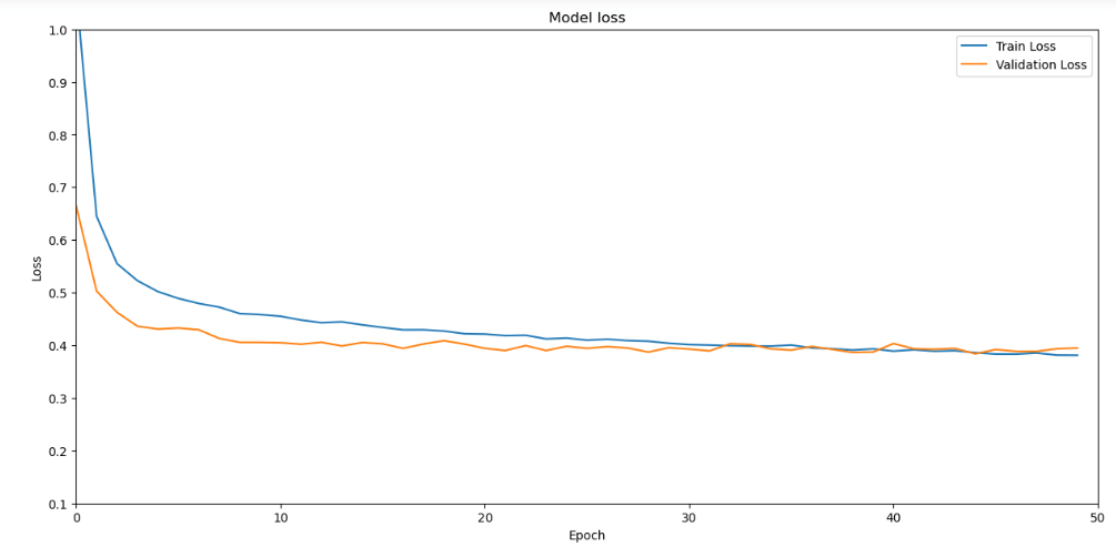
Summarize history for loss
plt.figure(figsize = (15,7))
plt.plot(model_history.history[‘loss’])
plt.plot(model_history.history[‘val_loss’])
plt.title(‘Model loss’)
plt.ylabel(‘Loss’)
plt.xlabel(‘Epoch’)
plt.legend([‘Train Loss’, ‘Validation Loss’], loc=’upper right’)
plt.xlim(0,50)
plt.ylim(0.1,1.0)
plt.show()
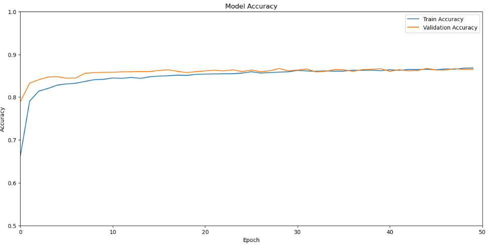
Summarize history for accuracy
plt.figure(figsize = (15,7))
plt.plot(model_history.history[‘accuracy’])
plt.plot(model_history.history[‘val_accuracy’])
plt.title(‘Model Accuracy’)
plt.ylabel(‘Accuracy’)
plt.xlabel(‘Epoch’)
plt.legend([‘Train Accuracy’, ‘Validation Accuracy’], loc=’upper right’)
plt.xlim(0,50)
plt.ylim(0.5,1.0)
plt.show()
Let’s evaluate the test score
scores_test = model_final.evaluate(X_test,y_test)
313/313 [==============================] - 0s 2ms/step - loss: 0.4227 - accuracy: 0.8564
scores_test = model_final.evaluate(X_test, y_test, verbose=2)
print(“Testing Accuracy: %.2f%%\n” % (scores_test[1] * 100))
313/313 - 0s - loss: 0.4227 - accuracy: 0.8564 - 424ms/epoch - 1ms/step
Testing Accuracy: 85.64%
Add a softmax layer to convert the model’s linear outputs logits to probabilities, which should be easier to interpret
probability_model = tf.keras.Sequential([model_final, tf.keras.layers.Softmax()])
Let’s make predictions
predictions = probability_model.predict(X_test)
313/313 [==============================] - 0s 709us/step
Model has predicted the label for each image in the testing set. Let’s take a look at the first prediction:
ii=1
predictions[ii]
array([0.08596796, 0.08593319, 0.22232993, 0.08594155, 0.08826148,
       0.08593146, 0.08782255, 0.08593164, 0.08594636, 0.08593389],
      dtype=float32)
np.argmax(predictions[ii])
2
y_test[ii]
2
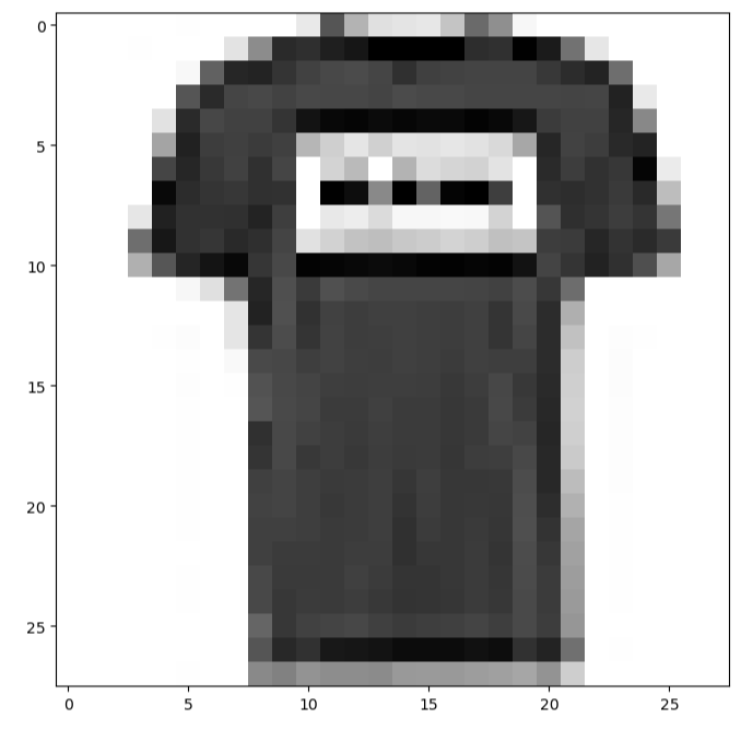
Let’s plot the test image
plt.figure(figsize = (8,8))
plt.imshow(X_test[ii],cmap = ‘Greys’);
![Test image y_test[2]](https://newdigitals.org/wp-content/uploads/2023/01/leeitem.png?w=663)
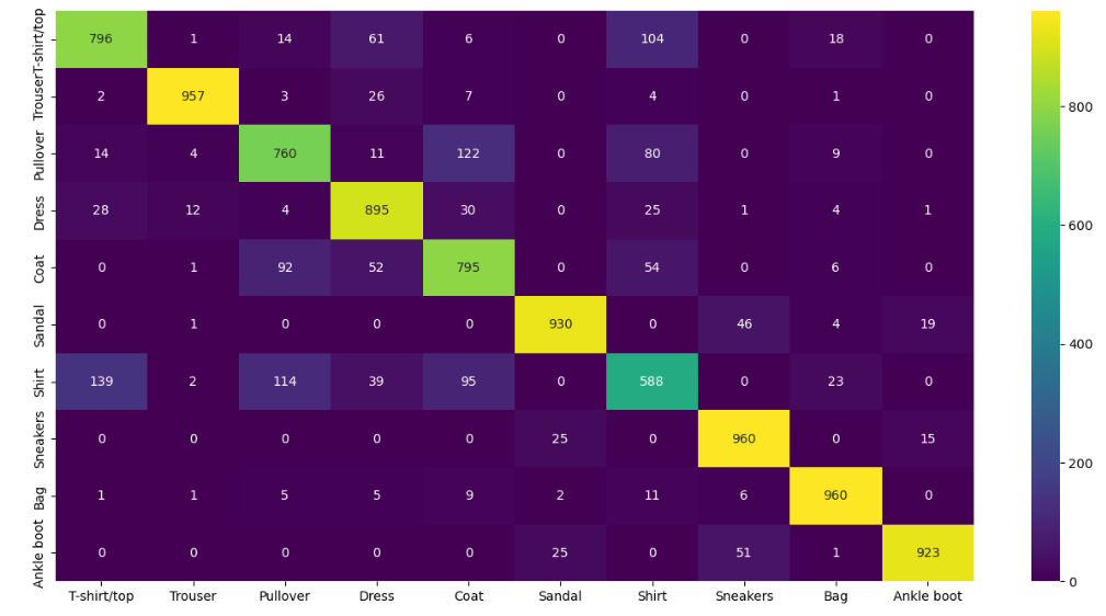
Let’s look at the multi-label confusion matrix
from sklearn.metrics import confusion_matrix
plt.figure(figsize = (16,8))
y_pred_labels = [np.argmax(label) for label in predictions]
cm = confusion_matrix(y_test,y_pred_labels)
HeatMap:
sns.heatmap(cm , annot = True,fmt = ‘d’,xticklabels = class_labels,yticklabels = class_labels,cmap = ‘viridis’);
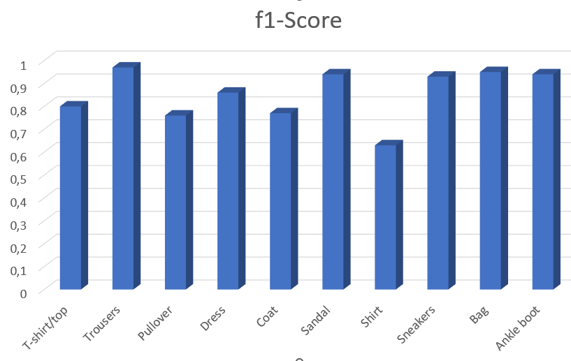
Let’s print the multi-label classification report
from sklearn.metrics import classification_report
report = classification_report (y_test,y_pred_labels,target_names = class_labels)
print(report)
        precision    recall  f1-score   support

 T-shirt/top       0.81      0.80      0.80      1000
     Trouser       0.98      0.96      0.97      1000
    Pullover       0.77      0.76      0.76      1000
       Dress       0.82      0.90      0.86      1000
        Coat       0.75      0.80      0.77      1000
      Sandal       0.95      0.93      0.94      1000
       Shirt       0.68      0.59      0.63      1000
    Sneakers       0.90      0.96      0.93      1000
         Bag       0.94      0.96      0.95      1000
  Ankle boot       0.96      0.92      0.94      1000

    accuracy                           0.86     10000
   macro avg       0.86      0.86      0.86     10000
weighted avg       0.86      0.86      0.86     10000
Conclusions
- In this post, we discussed how to address the multi-label image classification problem by implementing a CNN model using Keras, TensorFlow and GridSearchCV.
- Specifically, we discovered how to develop a CNN for clothing classification from scratch.
- We looked at the entire process of implementing a feedforward CNN model on the Fashion-MNIST dataset to classify images of clothing apparel on train data and make predictions on test data using GridSearchCV Hyperparameter tuning technique to achieve the best accuracy and performance.
- In this tutorial, you discovered how to develop a convolutional neural network for clothing classification from scratch.
- We have learned:
- How to develop a robust evaluation of a DL model and establish a baseline of performance for a multi-label image classification task.
- How to explore extensions to a baseline model to improve learning and model capacity via hyper-parameter tuning.
- How to develop a finalized model, evaluate the performance of the final model, and use it to make predictions on new images.
Explore More
Short-Term Stock Market Price Prediction using Deep Learning Models
Supervised ML/AI Stock Prediction using Keras LSTM Models
E-Commerce ML/AI Classification
E-Commerce Data Science Use-Case


Make a one-time donation
Make a monthly donation
Make a yearly donation
Choose an amount
Or enter a custom amount
Your contribution is appreciated.
Your contribution is appreciated.
Your contribution is appreciated.

Leave a comment