Contents:
Background
With the growing number of people looking to shop online, the e-commerce industry is expanding rapidly. In the context of this revolutionary growth, Data Science (DS) can maximize the value out of the vast amount of data available in online retail platforms like Amazon, bol or Shopify. The current DS priority focus is as follows:
- Product recommendation for users
- Analysis of customer trends/behaviors
- Forecasting sales and stock logistics
- Optimizing product pricing and payment methods.
The goal is to build a DS-based customer analytics platform that is focused on customer profiling/segmentation, sentiment/churn analysis, and CLV prediction. The actual implementation is referred to as the Exploratory Data Analytis (EDA) pipeline based upon the Pandas Python library. Pandas provides extensive means for EDA by importing data in table formates like .csv or .xlsx. It also provides a wide range of visualization options of interest to the Business Intelligence (BI) decision-making process.
The EDA Pipeline
Step 1: Import the necessary libraries
import pandas as pd
import matplotlib.pyplot as plt
import matplotlib.gridspec as gridspec
import seaborn as sns
import numpy as np
Step 2: Read the input tabular data and analyze the corresponding data frame
df = pd.read_csv(“$path/e_commerce.csv”),
where $path is the full path to the input file e_commerce.csv.
Explore the above data
df.info()
<class 'pandas.core.frame.DataFrame'>
RangeIndex: 550068 entries, 0 to 550067
Data columns (total 12 columns):
 #   Column                      Non-Null Count   Dtype
---  ------                      --------------   -----
 0   User_ID                     550068 non-null  int64
 1   Product_ID                  550068 non-null  object
 2   Gender                      550068 non-null  object
 3   Age                         550068 non-null  object
 4   Occupation                  550068 non-null  int64
 5   City_Category               550068 non-null  object
 6   Stay_In_Current_City_Years  550068 non-null  object
 7   Marital_Status              550068 non-null  int64
 8   Product_Category_1          550068 non-null  int64
 9   Product_Category_2          376430 non-null  float64
 10  Product_Category_3          166821 non-null  float64
 11  Purchase                    550068 non-null  int64
dtypes: float64(2), int64(5), object(5)
memory usage: 50.4+ MB
It consists of a series of transactions made in an e-commerce platform: User_ID, Product_Categories, etc.
Let us count null features in the dataset
df.isnull().sum()
User_ID                            0
Product_ID                         0
Gender                             0
Age                                0
Occupation                         0
City_Category                      0
Stay_In_Current_City_Years         0
Marital_Status                     0
Product_Category_1                 0
Product_Category_2            173638
Product_Category_3            383247
Purchase                           0
dtype: int64
As we can see, there are 173.638 null fields for product 2, meaning that the user did not purchase more than one in this case. Also, there are 383.247 null fields for product 3.
Let us replace the null features with 0 to have a clean dataset
df.fillna(0, inplace=True) # Re-check N/A was replaced with 0.
and group the data by User_ID to identify users that spend the most in our store
purchases = df.groupby([‘User_ID’]).sum().reset_index()
This yields
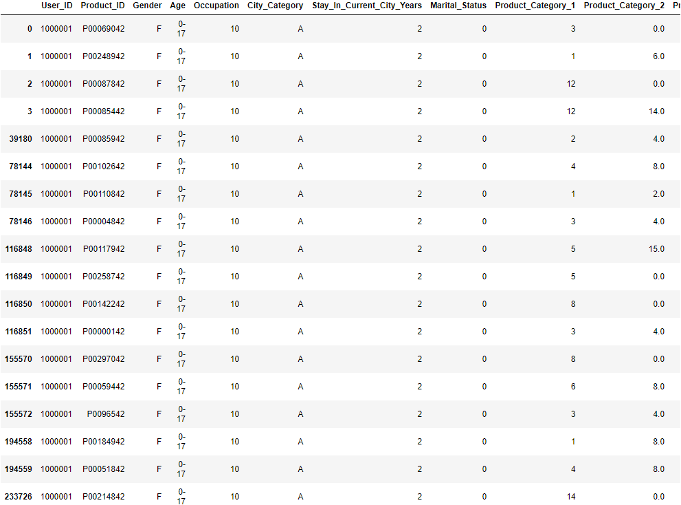
purchases.head()
df[df[‘User_ID’] == 1000001]

Let us look at the average sale versus the age group
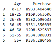
purchase_by_age = df.groupby(‘Age’)[‘Purchase’].mean().reset_index()
This yields
print(purchase_by_age)
print(purchase_by_age[‘Age’])

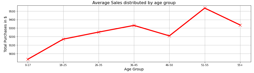
We can see that the group of users whose age ranges from 51–55 spends the most in the store. This means that CMO should focus on this group during the marketing campaign. Let’s take a look at the 2D plot Total Purchases (in $) versus Age Group:
plt.figure(figsize=(16,4))
plt.plot(purchase_by_age[‘Age’],purchase_by_age[‘Purchase’],color=’red’, marker=’x’,lw=4,markersize=12)
plt.grid()
plt.xlabel(‘Age Group’, fontsize=14)
plt.ylabel(‘Total Purchases in $’, fontsize=14)
plt.title(‘Average Sales distributed by age group’, fontsize=16)
plt.show()
We can also plot the histogram
plt.hist(purchase_by_age[‘Purchase’])
(array([1., 0., 0., 1., 1., 1., 2., 0., 0., 1.]),
 array([8933.46464044, 8993.5989795 , 9053.73331855, 9113.8676576 ,
        9174.00199665, 9234.1363357 , 9294.27067475, 9354.40501381,
        9414.53935286, 9474.67369191, 9534.80803096]),
 <BarContainer object of 10 artists>)

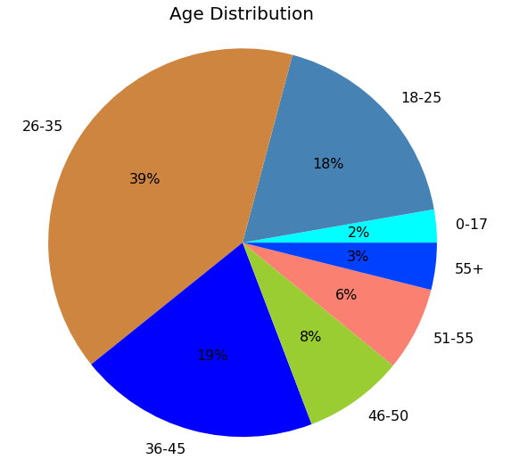
Let us find out which age group and gender make more transactions
age_and_gender = df.groupby(‘Age’)[‘Gender’].count().reset_index()
gender = df.groupby(‘Gender’)[‘Age’].count().reset_index()
Plot distribution
plt.figure(figsize=(12,9))
plt.pie(age_and_gender[‘Gender’], labels=age_and_gender[‘Age’],autopct=’%d%%’, colors=[‘cyan’, ‘steelblue’,’peru’,’blue’,’yellowgreen’,’salmon’,’#0040FF’],textprops={‘fontsize’: 16})
plt.axis(‘equal’)
plt.title(“Age Distribution”, fontsize=’20’)
plt.show()
plt.figure(figsize=(12,9))
plt.pie(gender[‘Age’], labels=gender[‘Gender’],autopct=’%d%%’, colors=[‘salmon’,’steelblue’],textprops={‘fontsize’: 16})
plt.axis(‘equal’)
plt.title(“Gender Distribution”, fontsize=’20’)
plt.show()

Also, we can calculate which occupations (labels 0-20) purchase more products in our store:
occupation = df.groupby(‘Occupation’)[‘Purchase’].mean().reset_index()
We can plot bar chart with the line plot:
sns.set(style=”white”, rc={“lines.linewidth”: 3})
fig, ax1 = plt.subplots(figsize=(12,9))
sns.barplot(x=occupation[‘Occupation’],y=occupation[‘Purchase’],color=’#004488′,ax=ax1)
sns.lineplot(x=occupation[‘Occupation’],y=occupation[‘Purchase’],color=’salmon’,marker=”o”,ax=ax1)
plt.axis([-1,21,8000,10000])
plt.title(‘Occupation Bar Chart’, fontsize=’15’)
plt.show()
sns.set()

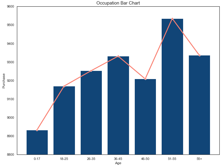
In addition, we can check the relationship purchase-age-occupation
occupation = df.groupby(‘Age’)[‘Purchase’].mean().reset_index()
Plot bar chart with line plot:
sns.set(style=”white”, rc={“lines.linewidth”: 3})
fig, ax1 = plt.subplots(figsize=(12,9))
sns.barplot(x=occupation[‘Age’],y=occupation[‘Purchase’],color=’#004488′,ax=ax1)
sns.lineplot(x=occupation[‘Age’],y=occupation[‘Purchase’],color=’salmon’,marker=”o”,ax=ax1)
plt.ylim([8800, 9600])
plt.title(‘Occupation Bar Chart’, fontsize=’15’)
plt.show()
sns.set()
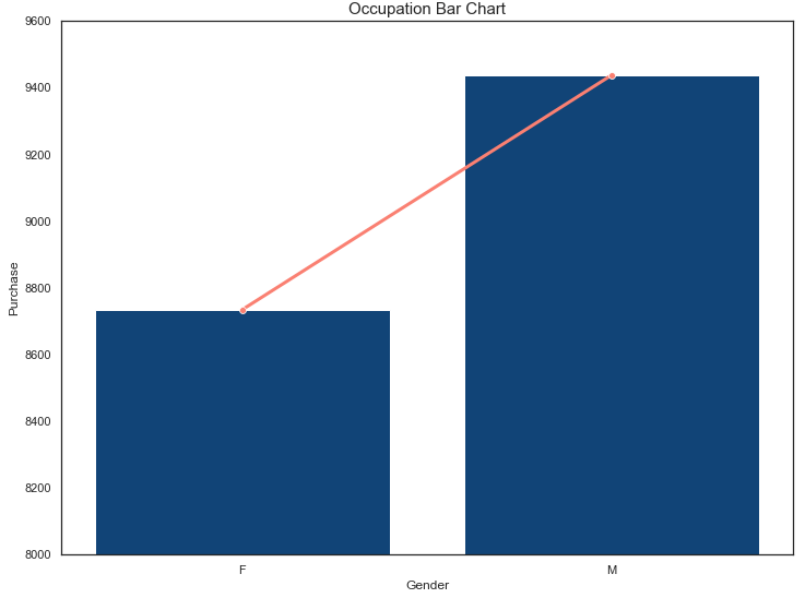
And the occupation-purchase-gender relationship is given by
occupation = df.groupby(‘Gender’)[‘Purchase’].mean().reset_index()
Plot bar chart with line plot:
sns.set(style=”white”, rc={“lines.linewidth”: 3})
fig, ax1 = plt.subplots(figsize=(12,9))
sns.barplot(x=occupation[‘Gender’],y=occupation[‘Purchase’],color=’#004488′,ax=ax1)
sns.lineplot(x=occupation[‘Gender’],y=occupation[‘Purchase’],color=’salmon’,marker=”o”,ax=ax1)
plt.ylim([8000, 9600])
plt.title(‘Occupation Bar Chart’, fontsize=’15’)
plt.show()
sns.set()
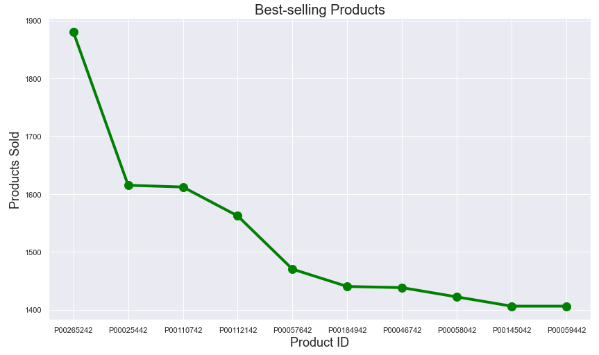
Finally, we can identify the best-selling products in the store:
product = df.groupby(‘Product_ID’)[‘Purchase’].count().reset_index()
product.rename(columns={‘Purchase’:’Count’},inplace=True)
product_sorted = product.sort_values(‘Count’,ascending=False)
Plot line plot
plt.figure(figsize=(14,8))
plt.plot(product_sorted[‘Product_ID’][:10], product_sorted[‘Count’][:10], linestyle=’-‘, color=’green’, marker=’o’,lw=4,markersize=12)
plt.title(“Best-selling Products”, fontsize=’20’)
plt.xlabel(‘Product ID’, fontsize=’18’)
plt.ylabel(‘Products Sold’, fontsize=’18’)
plt.show()
Bottom Line
This Python EDA use-case explains why DS pipelines have found so many commercially viable applications in the e-commerce and retail industry (recommendation engines, Market Basket Analysis, Warranty Analytics, Price Optimization, Inventory Management, location of new stores, customer sentiment analysis, Merchandising, CLV prediction, etc.). These pipelines can predict the purchases, profits, losses and even nudge customers into buying additional products on the basis of their behaviour. Organizations also can use purchase data to create psychological portraits of a customer to market products to them and use it to drive customer loyalty and thereby increase ROI.


Leave a comment