E-Commerce ML/AI Classification

Contents:

1. Introduction
2. Data Pre-Processing
3. Build the Training ML Model
4. Make ML Predictions

Introduction

Let us look at the most popular supervised ML/AI use-case – classification of various clothing images to categorize clothing into several categories. The classification of fashion items in a photograph includes the identification of individual garments. The same has applications in social networking (Instagram, YouTube, Twitter, etc.), e-commerce (e.g. Shopify), and criminal law as well.

Classifying clothing images will be done in Python, Jupyter Anaconda IDE with the help of TensorFlow (TF). The ML algorithm uses tf.keras, a high-level API to build and train models in TF. It trains a neural network model to classify images of clothing, like sneakers and shirts. We’ll be working with TF along with numpy and matplotlib:

import tensorflow as tf
import numpy as np
import matplotlib.pyplot as plt

Data Pre-Processing

The single code line below achieves the loading of input data:

fashion_data=tf.keras.datasets.fashion_mnist

We divide the input data into two parts based on the 80-20 rule: 80% of the data is sent to training data and 20% to testing data. The code below normalizes the data by 255.0 and splits the normalized data into training/testing subsets:

(inp_train,out_train),(inp_test,out_test)=fashion_data.load_data()
inp_train = inp_train/255.0
inp_test = inp_test/255.0

Let’s check the shape of these two subsets:

print(“Shape of Input Training Data: “, inp_train.shape)
print(“Shape of Output Training Data: “, out_train.shape)
print(“Shape of Input Testing Data: “, inp_test.shape)
print(“Shape of Output Testing Data: “, out_test.shape)

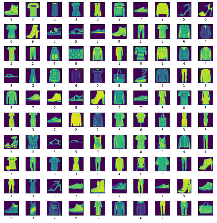
Shape of Input Training Data:  (60000, 28, 28)
Shape of Output Training Data:  (60000,)
Shape of Input Testing Data:  (10000, 28, 28)
Shape of Output Testing Data:  (10000,)

Notice that this dataset includes 60,000 photos in grayscale, each measuring 28x28 pixels, from ten different fashion categories, plus a dummy set of 10,000 images.
Let us plot the data as follows:

plt.figure(figsize=(10,10))
for i in range(100):
plt.subplot(10,10,i+1)
plt.imshow(inp_train[i])
plt.xticks([])
plt.yticks([])
plt.xlabel(out_train[i])
plt.tight_layout()
plt.show()

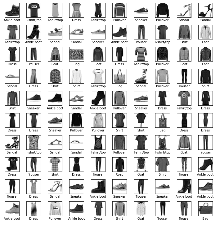
Let us change the labels to actual well-defined names and plot the result as b/w images:

Labels=[‘T-shirt/top’, ‘Trouser’, ‘Pullover’, ‘Dress’, ‘Coat’,’Sandal’, ‘Shirt’, ‘Sneaker’, ‘Bag’, ‘Ankle boot’]
plt.figure(figsize=(10,10))
for i in range(100):
plt.subplot(10,10,i+1)
plt.xticks([])
plt.yticks([])
plt.imshow(inp_train[i], cmap=plt.cm.binary)
plt.xlabel(Labels[out_train[i]])
plt.tight_layout()
plt.show()

Build the Training ML Model

We build, compile and train the ML model using the following code:

my_model = tf.keras.Sequential([
tf.keras.layers.Flatten(input_shape=(28, 28)),
tf.keras.layers.Dense(n256, activation=’relu’),
tf.keras.layers.Dense(n20)
])
my_model.compile(optimizer=’adam’,
loss=tf.keras.losses.SparseCategoricalCrossentropy(from_logits=True),
metrics=[‘accuracy’])
my_model.fit(inp_train, out_train, epochs=e20),

where n20=20 and n256=256 are NN dense layer parameters, e20=20 is the number of epochs, layer activation functions are relu, tanh, and sigmoid, and the optimizer list is given below

• SGD
• RMSprop
• Adam
• Adadelta
• Adagrad
• Adamax
• Nadam
• Ftrl

All built-in metrics are passed via their string identifier (in this case, default constructor argument values are used, including a default metric name), e.g.

model.compile(
    optimizer='adam',
    loss='mean_squared_error',
    metrics=[
        'MeanSquaredError',
        'AUC',
    ]
)

Let us run the code with the following parameters:

my_model = tf.keras.Sequential([
tf.keras.layers.Flatten(input_shape=(28, 28)),
tf.keras.layers.Dense(256, activation=’relu’),
tf.keras.layers.Dense(20)
])
my_model.compile(optimizer=’adam’,
loss=tf.keras.losses.SparseCategoricalCrossentropy(from_logits=True),
metrics=[‘accuracy’])
my_model.fit(inp_train, out_train, epochs=20)

The output is

loss: 0.1625 - accuracy: 0.9381

Benchmarking test: the Ftrl optimizer yields

loss: 0.6558 - accuracy: 0.7621

Let us check the final loss and accuracy values

313/313 - 0s - loss: 0.3325 - accuracy: 0.8948 - 182ms/epoch - 583us/step

Accuracy: 89.48000073432922

The final accuracy of our trained ML model is 89.48% which is acceptable.

Make ML Predictions

We are ready to make ML predictions using our trained model:

prob=tf.keras.Sequential([my_model,tf.keras.layers.Softmax()])
pred=prob.predict(inp_test)

Let us plot the first 30 classified b/w clothing images

Further improvements can be accomplished by changing the TF training parameters (optimizer, activation, ep20, n20,n256, etc.) and running benchmarking tests, as shown above.