Walmart Weekly Sales Time Series Forecasting using SARIMAX & ML Models

This blog post is a deep dive into Time Series Forecasting (TSF) using SARIMAX and Supervised Machine Learning (ML) algorithms.
The objective is to explain nuts & bolts of these powerful TSF techniques while evaluating and comparing their performance.
Referring to the earlier studies [1], [2] & [3], we will predict Walmart weekly store sales using the Kaggle dataset.
With more than 245 million customers visiting 10,900 stores and with 10 active websites across the globe, Walmart is definitely a name to reckon with in the retail sector.
According to the data, Walmart’s net sales were forecast to be around 547 billion U.S. dollars in 2021, following the upsurge in 2020 that was driven by COVID-19. From 2021 onwards, Walmart’s net sales were forecast to increase with each consecutive year. By 2026, it was forecast that Walmart’s net sales would grow to 675.2 billion U.S. dollars, which includes store-based and e-commerce net sales.
Our aim is to understand how different factors affect the Walmart sales by creating more efficient strategies of increasing revenues.
Walmart Recruiting: We are provided with historical sales data for 45 Walmart stores located in different regions. Each store contains a number of departments, and we are tasked with predicting the department-wide sales for each store.
In addition, Walmart runs several promotional markdown events throughout the year. These markdowns precede prominent holidays, the four largest of which are the Super Bowl, Labor Day, Thanksgiving, and Christmas. The weeks including these holidays are weighted five times higher in the evaluation than non-holiday weeks.

TSF is a great strategy for predicting future sales using historical data. In an auto regressive (AR) model the model predicts the next data point by looking at previous data points and using a linear regression. ARIMA stands for auto regressive integrated moving average. SARIMAX is similar and stands for seasonal auto regressive integrated moving average with exogenous factors.
In fact, the crucial point of this study is to combine SARIMAX and supervised ML into a single framework to optimized the advantages of each.
Specifically, how ML helps in sales forecasting? SARIMAX methods require time-consuming manual work and data engineering, which can be difficult and expensive. ML, on the other hand, is able to automatically learn from data and make predictions without any human intervention.
Here are some advantages you can anticipate if you introduce ML into your sales forecasting process:
- Better Sales Forecasting Accuracy
- Providing New Insights into Customer Behavior
- Saving Time and Resources (with excellent reporting capabilities)
- Spotting New Insights Through Uncovering Patterns.

Table of Contents

Input Data Preparation
Feature Correlation Matrix
Seasonal Decomposition
SARIMAX Diagnostics
One-Step Ahead Forecast
Dynamic Forecast
Feature Engineering
Linear Regression
Random Forest
KNN Regressor
XGBoost Model
Final Comparison
Summary
Explore More
References

Let’s start by installing/importing our libraries and preparing input data to get things going!
Read more here and follow the notebook.

Input Data Preparation

Setting the working directory YOURPATH

import os
os.chdir('YOURPATH')    # Set working directory
os. getcwd()

Installing and importing libraries

!pip install xgboost
!pip install catboost
!pip install lightgbm

import sklearn; 
print(sklearn.__version__)
1.4.0

import warnings
import itertools
import numpy as np
import scipy.stats as stats
import warnings
warnings.filterwarnings("ignore")
import seaborn as sns
import matplotlib.pyplot as plt
import pandas as pd
import calendar
from sklearn.model_selection import cross_val_score, cross_val_predict
from sklearn import metrics
from sklearn.preprocessing import StandardScaler
from sklearn.linear_model import Lasso, LinearRegression, LassoCV
from sklearn.model_selection import train_test_split, cross_val_score
from sklearn.neighbors import KNeighborsRegressor
import random
import sqlite3
from itertools import cycle, islice
from sklearn.tree import DecisionTreeRegressor
from sklearn.ensemble import RandomForestRegressor
from sklearn.ensemble import GradientBoostingRegressor
import xgboost as xgb
import catboost as cb
import lightgbm as lgb
from sklearn.experimental import enable_hist_gradient_boosting
from sklearn.ensemble import HistGradientBoostingRegressor
from sklearn.svm import SVR
# Import timedelta from datetime library
from datetime import timedelta

ss = StandardScaler()

Reading the input data

walmart = pd.read_csv('train.csv')

walmart_feature = pd.read_csv('features.csv')

walmart_store = pd.read_csv('stores.csv')

Grouping, merging, encoding categorical variables, fill NaN, and converting “Date” to date time

walmart_store_group=walmart.groupby(["Store","Date"])[["Weekly_Sales"]].sum()
walmart_store_group.reset_index(inplace=True)
result = pd.merge(walmart_store_group, walmart_store, how='inner', on='Store', left_on=None, right_on=None,
        left_index=False, right_index=False, sort=False,
        suffixes=('_x', '_y'), copy=True, indicator=False)

data = pd.merge(result, walmart_feature, how='inner', on=['Store','Date'], left_on=None, right_on=None,
        left_index=False, right_index=False, sort=False,
        suffixes=('_x', '_y'), copy=True, indicator=False)
#let's encode the categorical column : IsHoliday

data['IsHoliday'] = data['IsHoliday'].apply(lambda x: 1 if x == True else 0)
# Now converting "Date"  to date time
data["Date"]=pd.to_datetime(data.Date)

# Extracting details from date given. so that can be used for seasonal checks or grouping

data["Day"]=data.Date.dt.day
data["Month"]=data.Date.dt.month
data["Year"]=data.Date.dt.year

# Changing the Months value from numbers to real values like Jan, Feb to Dec
data['Month'] = data['Month'].apply(lambda x: calendar.month_abbr[x])
#will create this column for later use
data['MarkdownsSum'] = data['MarkDown1'] + data['MarkDown2'] + data['MarkDown3'] + data['MarkDown4'] + data['MarkDown5'] 
data.fillna(0, inplace = True)
data['Week'] = data.Date.dt.isocalendar().week

Selecting stores 4 and 6

data1 = pd.read_csv('train.csv')
data1.set_index('Date', inplace=True)

store4 = data1[data1.Store == 4]
# there are about 45 different stores in this dataset.

sales4 = pd.DataFrame(store4.Weekly_Sales.groupby(store4.index).sum())
sales4.dtypes
sales4.head(20)
# Grouped weekly sales by store 4

#remove date from index to change its dtype because it clearly isnt acceptable.
sales4.reset_index(inplace = True)

#converting 'date' column to a datetime type
sales4['Date'] = pd.to_datetime(sales4['Date'])
# resetting date back to the index
sales4.set_index('Date',inplace = True)
# Lets take store 6 data for analysis
store6 = data1[data1.Store == 6]
# there are about 45 different stores in this dataset.

sales6 = pd.DataFrame(store6.Weekly_Sales.groupby(store6.index).sum())
sales6.dtypes
# Grouped weekly sales by store 6

#remove date from index to change its dtype because it clearly isnt acceptable.
sales6.reset_index(inplace = True)

#converting 'date' column to a datetime type
sales6['Date'] = pd.to_datetime(sales6['Date'])
# resetting date back to the index
sales6.set_index('Date',inplace = True)

Feature Correlation Matrix

Plotting the feature correlation matrix

sns.set(style="white")

corr = data.corr()
mask = np.triu(np.ones_like(corr))
f, ax = plt.subplots(figsize=(20, 10))
cmap = sns.diverging_palette(220, 10, as_cmap=True)
plt.title('Correlation Matrix', fontsize=14)
sns.heatmap(corr, mask=mask, cmap=cmap, vmax=1, center=0,
            square=True, linewidths=.5, cbar_kws={"shrink": .5}, annot=True)

plt.show()

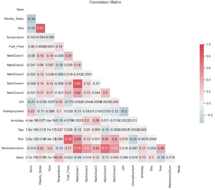
The correlation matrix is a matrix that shows the correlation between variables. It gives the correlation between all the possible pairs of values in a matrix format. Using the above matrix, we can evaluate the relationship between our variables.
In ML, highly correlated features refer to variables that have a strong linear relationship with each other. The presence of highly correlated features can lead to several issues, and removing them is often beneficial.

Seasonal Decomposition

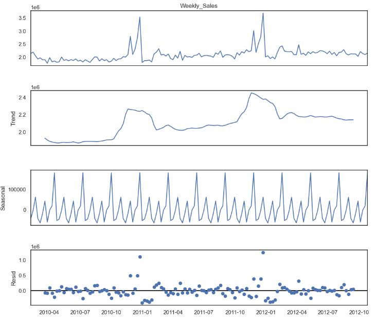
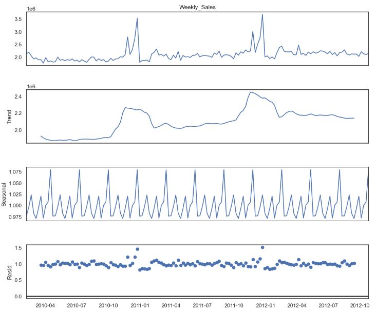
Let’s look at the time series additive/multiplicative decomposition. It helps us disentangle our input data into components that may be easier to forecast. Basically, a time series consists of four components: level, trend, seasonality, and noise.

from statsmodels.tsa.seasonal import seasonal_decompose

decomposition = seasonal_decompose(sales4.Weekly_Sales, period=12)  
fig = plt.figure()  
fig = decomposition.plot()  
fig.set_size_inches(12, 10)
plt.show()

Additive seasonal decomposition of sales store 4.

decomposition = seasonal_decompose(sales4.Weekly_Sales, model= 'multiplicative', period=12)  
fig = plt.figure()  
fig = decomposition.plot()  
fig.set_size_inches(12, 10)
plt.show()

Multiplicative seasonal decomposition of sales store 4.

SARIMAX Diagnostics

Let’s examine the Statsmodels’ SARIMAX (Seasonal AutoRegressive Integrated Moving Average) model with exogenous regressors.

# Define the p, d and q parameters to take any value between 0 and 2
p = d = q = range(0, 5)

# Generate all different combinations of p, d and q triplets
pdq = list(itertools.product(p, d, q))

# Generate all different combinations of seasonal p, d and q triplets
seasonal_pdq = [(x[0], x[1], x[2], 52) for x in list(itertools.product(p, d, q))]

import statsmodels.api as sm

mod = sm.tsa.statespace.SARIMAX(y1,
                                order=(4, 4, 3),
                                seasonal_order=(1, 1, 0, 52),   #enforce_stationarity=False,
                                enforce_invertibility=False)

results = mod.fit()

print(results.summary().tables[1])

==============================================================================
                 coef    std err          z      P>|z|      [0.025      0.975]
------------------------------------------------------------------------------
ar.L1         -1.7449      0.544     -3.207      0.001      -2.811      -0.679
ar.L2         -1.2798      0.586     -2.185      0.029      -2.428      -0.132
ar.L3         -0.5894      0.252     -2.340      0.019      -1.083      -0.096
ar.L4         -0.1879      0.092     -2.036      0.042      -0.369      -0.007
ma.L1         -1.3853      0.494     -2.805      0.005      -2.353      -0.417
ma.L2         -0.2065      1.063     -0.194      0.846      -2.290       1.877
ma.L3          0.5960      0.593      1.005      0.315      -0.566       1.758
ar.S.L52      -0.0672      0.048     -1.391      0.164      -0.162       0.027
sigma2      1.622e+10   6.23e-11    2.6e+20      0.000    1.62e+10    1.62e+10
==============================================================================

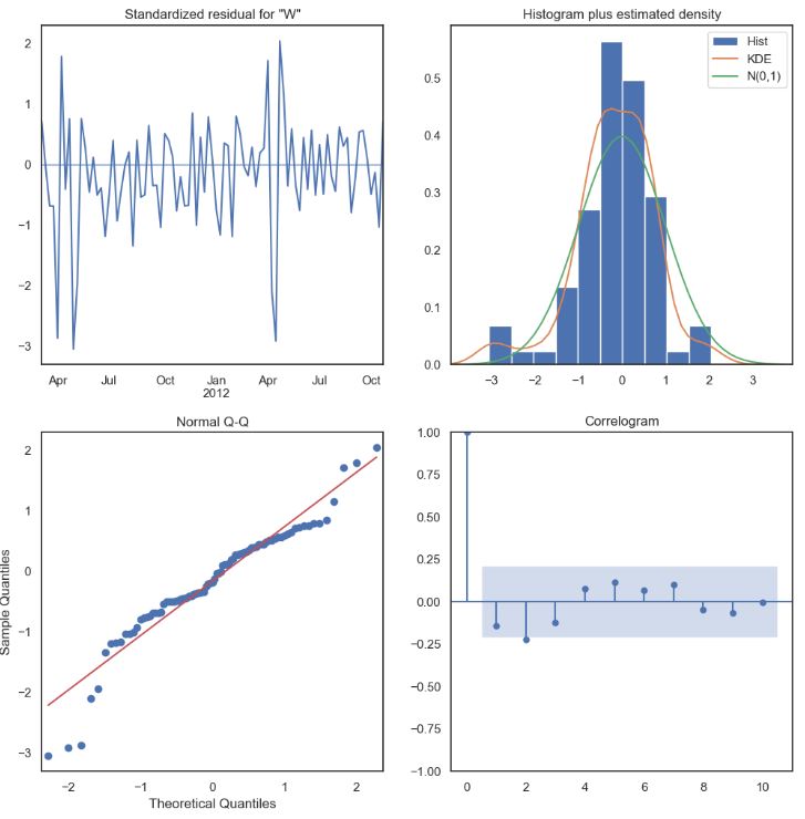
Plotting SARIMAX QC diagnostics (standardized residuals, Histogram plus estimated density, Q-Q plot, and correlogram)

results.plot_diagnostics(figsize=(12, 12))
plt.show()

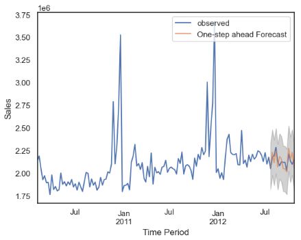
SARIMAX QC diagnostics (standardized residuals, Histogram plus estimated density, Q-Q plot, and correlogram)

One-Step Ahead Forecast

Let’s perform one-step ahead TSF for last 90 days

# Will predict for last 90 days. So setting the date according to that
pred = results.get_prediction(start=pd.to_datetime('2012-07-27'), dynamic=False)
pred_ci = pred.conf_int()
ax = y1['2010':].plot(label='observed')
pred.predicted_mean.plot(ax=ax, label='One-step ahead Forecast', alpha=.7)

ax.fill_between(pred_ci.index,
                pred_ci.iloc[:, 0],
                pred_ci.iloc[:, 1], color='k', alpha=.2)

ax.set_xlabel('Time Period')
ax.set_ylabel('Sales')
plt.legend()

plt.show()

y_forecasted = pred.predicted_mean
y_truth = y1['2012-7-27':]

# Compute the mean square error
mse = ((y_forecasted - y_truth) ** 2).mean()
print('The Mean Squared Error of our forecasts is {}'.format(round(mse, 2)))
The Mean Squared Error of our forecasts is 4757741704.39

Dynamic Forecast

Performing the dynamic SARIMAX forecast

pred_dynamic = results.get_prediction(start=pd.to_datetime('2012-7-27'), dynamic=True, full_results=True)
pred_dynamic_ci = pred_dynamic.conf_int()
ax = y1['2010':].plot(label='observed', figsize=(12, 8))
pred_dynamic.predicted_mean.plot(label='Dynamic Forecast', ax=ax)

ax.fill_between(pred_dynamic_ci.index,
                pred_dynamic_ci.iloc[:, 0],
                pred_dynamic_ci.iloc[:, 1], color='k', alpha=.25)

ax.fill_betweenx(ax.get_ylim(), pd.to_datetime('2012-7-26'), y1.index[-1],
                 alpha=.1, zorder=-1)

ax.set_xlabel('Time Period')
ax.set_ylabel('Sales')

plt.legend()
plt.show()

# Extract the predicted and true values of our time series
y_forecasted = pred_dynamic.predicted_mean

y_truth = y1['2012-7-27':]

# Compute the Root mean square error
rmse = np.sqrt(((y_forecasted - y_truth) ** 2).mean())
print('The Root Mean Squared Error of our forecasts is {}'.format(round(rmse, 2)))
The Root Mean Squared Error of our forecasts is 77410.45

Residual= y_forecasted - y_truth
print("Residual for Store 4",np.abs(Residual).sum())
Residual for Store4 854828.1737922677

Feature Engineering

Let’s prepare our data for training supervised ML models.
Data pre-processing

#Importing Modules
import numpy as np
import pandas as pd

import matplotlib.pyplot as plt
import seaborn as sns

from scipy import stats
import statsmodels.api as sm

from sklearn.preprocessing import MinMaxScaler

import pickle 
from os import path

from sklearn import metrics
from sklearn.model_selection import train_test_split 
from sklearn.linear_model import LinearRegression
from sklearn.ensemble import RandomForestRegressor
from sklearn.neighbors import KNeighborsRegressor
from xgboost import XGBRegressor

from keras.models import Sequential
from keras.layers import Dens
from scikeras.wrappers import KerasRegressor

#Importing Datasets
data = pd.read_csv('train.csv')
stores = pd.read_csv('stores.csv')
features = pd.read_csv('features.csv')

#Handling missing values of features dataset
features["CPI"].fillna(features["CPI"].median(),inplace=True)
features["Unemployment"].fillna(features["Unemployment"].median(),inplace=True)
for i in range(1,6):
  features["MarkDown"+str(i)] = features["MarkDown"+str(i)].apply(lambda x: 0 if x < 0 else x)
  features["MarkDown"+str(i)].fillna(value=0,inplace=True)

#Merging Training Dataset and merged stores-features Dataset
data = pd.merge(data,stores,on='Store',how='left')
data = pd.merge(data,features,on=['Store','Date'],how='left')
data['Date'] = pd.to_datetime(data['Date'])
data.sort_values(by=['Date'],inplace=True)
data.set_index(data.Date, inplace=True)
data['IsHoliday_x'].isin(data['IsHoliday_y']).all()
True

data.drop(columns='IsHoliday_x',inplace=True)
data.rename(columns={"IsHoliday_y" : "IsHoliday"}, inplace=True)

#Splitting Date Column
data['Year'] = data['Date'].dt.year
data['Month'] = data['Date'].dt.month
data['Week'] = data['Date'].dt.week

#Outlier Detection and Abnormalities
agg_data = data.groupby(['Store', 'Dept']).Weekly_Sales.agg(['max', 'min', 'mean', 'median', 'std']).reset_index()
agg_data.isnull().sum()
Store      0
Dept       0
max        0
min        0
mean       0
median     0
std       37
dtype: int64

store_data = pd.merge(left=data,right=agg_data,on=['Store', 'Dept'],how ='left')
store_data.dropna(inplace=True)
data = store_data.copy()
del store_data
data['Total_MarkDown'] = data['MarkDown1']+data['MarkDown2']+data['MarkDown3']+data['MarkDown4']+data['MarkDown5']
data.drop(['MarkDown1','MarkDown2','MarkDown3','MarkDown4','MarkDown5'], axis = 1,inplace=True)
numeric_col = ['Weekly_Sales','Size','Temperature','Fuel_Price','CPI','Unemployment','Total_MarkDown']
data_numeric = data[numeric_col].copy()
data = data[(np.abs(stats.zscore(data_numeric)) < 2.5).all(axis = 1)]
data=data[data['Weekly_Sales']>=0]
data['IsHoliday'] = data['IsHoliday'].astype('int')

Data transformations for ML training

#One-hot-encoding
cat_col = ['Store','Dept','Type']
data_cat = data[cat_col].copy()
data_cat = pd.get_dummies(data_cat,columns=cat_col)
data = pd.concat([data, data_cat],axis=1)
data.drop(columns=cat_col,inplace=True)
data.drop(columns=['Date'],inplace=True)
#Data Normalization
num_col = ['Weekly_Sales','Size','Temperature','Fuel_Price','CPI','Unemployment','Total_MarkDown','max','min','mean','median','std']
minmax_scale = MinMaxScaler(feature_range=(0, 1))
def normalization(df,col):
  for i in col:
    arr = df[i]
    arr = np.array(arr)
    df[i] = minmax_scale.fit_transform(arr.reshape(len(arr),1))
  return df     
data = normalization(data.copy(),num_col)
#Recursive Feature Elimination
feature_col = data.columns.difference(['Weekly_Sales'])

Calculating feature importance weights with Random Forest

radm_clf = RandomForestRegressor(oob_score=True,n_estimators=23)
radm_clf.fit(data[feature_col], data['Weekly_Sales'])
RandomForestRegressor(n_estimators=23, oob_score=True)

indices = np.argsort(radm_clf.feature_importances_)[::-1]
feature_rank = pd.DataFrame(columns = ['rank', 'feature', 'importance'])

for f in range(data[feature_col].shape[1]):
    feature_rank.loc[f] = [f+1,
                           data[feature_col].columns[indices[f]],
                           radm_clf.feature_importances_[indices[f]]]

feature_rank
rank	feature	importance
0	1	median	5.239332e-01
1	2	mean	4.041693e-01
2	3	Week	1.983558e-02
3	4	Temperature	8.796048e-03
4	5	max	5.982970e-03
...	...	...	...
139	140	Dept_51	3.261420e-10
140	141	Dept_45	2.666958e-10
141	142	Dept_78	2.447811e-12
142	143	Dept_39	2.938813e-14
143	144	Dept_43	1.407660e-15
144 rows × 3 columns

x=feature_rank.loc[0:22,['feature']]
x=x['feature'].tolist()
print(x)
['median', 'mean', 'Week', 'Temperature', 'max', 'CPI', 'Fuel_Price', 'min', 'Unemployment', 'std', 'Month', 'Total_MarkDown', 'Dept_16', 'Dept_18', 'IsHoliday', 'Dept_3', 'Size', 'Dept_9', 'Dept_11', 'Year', 'Dept_1', 'Dept_5', 'Dept_56']

Creating X, Y columns and splitting them with test_size=0.30

X = data[x]
Y = data['Weekly_Sales']
data = pd.concat([X,Y],axis=1)
#Data Split
X = data.drop(['Weekly_Sales'],axis=1)
Y = data.Weekly_Sales
X_train,X_test,y_train,y_test = train_test_split(X,Y,test_size=0.30, random_state=50)

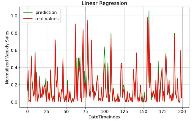
Linear Regression

Training the Linear Regression (LR) model

#Linear Regression Model
lr = LinearRegression()
lr.fit(X_train, y_train)
lr_acc = lr.score(X_test,y_test)*100
print("Linear Regressor Accuracy - ",lr_acc)
Linear Regressor Accuracy -  92.23004968201279
y_pred = lr.predict(X_test)
print("MAE" , metrics.mean_absolute_error(y_test, y_pred))
print("MSE" , metrics.mean_squared_error(y_test, y_pred))
print("RMSE" , np.sqrt(metrics.mean_squared_error(y_test, y_pred)))
print("R2" , metrics.explained_variance_score(y_test, y_pred))
MAE 0.03010877755242702
MSE 0.0035040752885774932
RMSE 0.059195230285703705
R2 0.9223007841955709

Plotting LR prediction vs real values

plt.figure(figsize=(10,6))
plt.rcParams.update({'font.size': 14})
plt.plot(lr.predict(X_test[:200]), label="prediction", linewidth=2.0,color='green')
plt.plot(y_test[:200].values, label="real values", linewidth=2.0,color='red')
plt.xlabel('DateTimeIndex')
plt.ylabel('Normalized Weekly Sales')
plt.title('Linear Regression')
plt.legend(loc="best")
plt.savefig('lr_real_pred.png')
plt.grid()
plt.show()

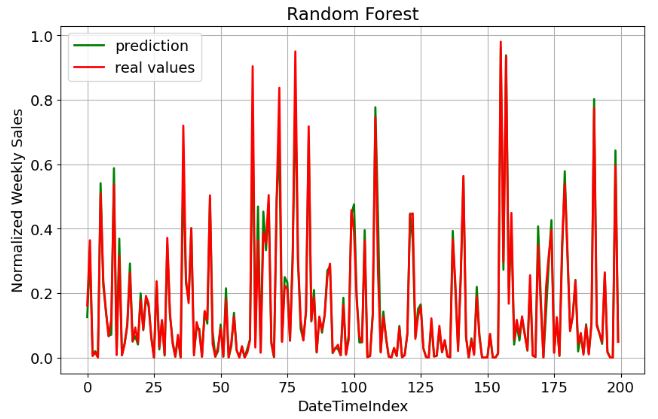
Linear Regression prediction vs real values

Random Forest

Training the Random Forest (RF) model

#Random Forest Regressor Model
rf = RandomForestRegressor()
rf.fit(X_train, y_train)
rf_acc = rf.score(X_test,y_test)*100
print("Random Forest Regressor Accuracy - ",rf_acc)
Random Forest Regressor Accuracy -  97.75107356196521
y_pred = rf.predict(X_test)
print("MAE" , metrics.mean_absolute_error(y_test, y_pred))
print("MSE" , metrics.mean_squared_error(y_test, y_pred))
print("RMSE" , np.sqrt(metrics.mean_squared_error(y_test, y_pred)))
print("R2" , metrics.explained_variance_score(y_test, y_pred))
MAE 0.015971949755612464
MSE 0.001014215951819333
RMSE 0.03184675732031965
R2 0.9775111310889105

Plotting RF prediction vs real values

plt.figure(figsize=(10,6))
plt.rcParams.update({'font.size': 14})
plt.plot(rf.predict(X_test[:200]), label="prediction", linewidth=2.0,color='green')
plt.plot(y_test[:200].values, label="real values", linewidth=2.0,color='red')
plt.xlabel('DateTimeIndex')
plt.ylabel('Normalized Weekly Sales')
plt.title('Random Forest')
plt.legend(loc="best")
plt.savefig('rf_real_pred.png')
plt.grid()
plt.show()

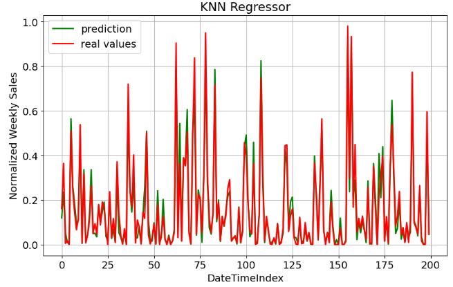
KNN Regressor

Training the KNN regression model

#K Neighbors Regressor Model
knn = KNeighborsRegressor(n_neighbors = 5,weights = 'uniform')
knn.fit(X_train,y_train)
knn_acc = knn.score(X_test, y_test)*100
print("KNeigbhbors Regressor Accuracy - ",knn_acc)
KNeigbhbors Regressor Accuracy -  92.17276485694632
y_pred = knn.predict(X_test)
print("MAE" , metrics.mean_absolute_error(y_test, y_pred))
print("MSE" , metrics.mean_squared_error(y_test, y_pred))
print("RMSE" , np.sqrt(metrics.mean_squared_error(y_test, y_pred)))
print("R2" , metrics.explained_variance_score(y_test, y_pred))
MAE 0.032121861389530305
MSE 0.00352990947434587
RMSE 0.05941304128174108
R2 0.9231507700958216

Plotting KNN prediction vs real values

plt.figure(figsize=(10,6))
plt.rcParams.update({'font.size': 14})
plt.plot(knn.predict(X_test[:200]), label="prediction", linewidth=2.0,color='green')
plt.plot(y_test[:200].values, label="real values", linewidth=2.0,color='red')
plt.xlabel('DateTimeIndex')
plt.ylabel('Normalized Weekly Sales')
plt.title('KNN Regressor')
plt.legend(loc="best")
plt.savefig('knn_real_pred.png')
plt.grid()
plt.show()

KNN regression prediction vs real values

XGBoost Model

Training the XGBoost model

#XGboost Model
xgbr = XGBRegressor()
xgbr.fit(X_train, y_train)
xgb_acc = xgbr.score(X_test,y_test)*100
print("XGBoost Regressor Accuracy - ",xgb_acc)
XGBoost Regressor Accuracy -  97.2773959867016
y_pred = xgbr.predict(X_test)
print("MAE" , metrics.mean_absolute_error(y_test, y_pred))
print("MSE" , metrics.mean_squared_error(y_test, y_pred))
print("RMSE" , np.sqrt(metrics.mean_squared_error(y_test, y_pred)))
print("R2" , metrics.explained_variance_score(y_test, y_pred))
MAE 0.019891003307968013
MSE 0.001227834034085841
RMSE 0.035040462812095406
R2 0.9727743194280883

Plotting XGBoost prediction vs real values

plt.figure(figsize=(10,6))
plt.rcParams.update({'font.size': 14})
plt.plot(xgbr.predict(X_test[:200]), label="prediction", linewidth=2.0,color='green')
plt.plot(y_test[:200].values, label="real values", linewidth=2.0,color='red')
plt.xlabel('DateTimeIndex')
plt.ylabel('Normalized Weekly Sales')
plt.title('XGboost Regression')
plt.legend(loc="best")
plt.savefig('rf_real_pred.png')
plt.grid()
plt.show()

XGBoost regression prediction vs real values

Final Comparison

Summarizing our ML comparisons as follows

acc = {'model':['lr_acc','rf_acc','knn_acc','xgb_acc'],'accuracy':[lr_acc,rf_acc,knn_acc,xgb_acc]}
acc_df = pd.DataFrame(acc)
acc_df
model	accuracy
0	lr_acc	92.230050
1	rf_acc	97.751074
2	knn_acc	92.172765
3	xgb_acc	97.277396  
plt.figure(figsize=(10,8))
sns.barplot(x='model',y='accuracy',data=acc_df)
plt.savefig('compared_models.png')
plt.show()

Accuracy of 4 ML models: LR, RF, KNN, and XGB.

Random Forest (RF) seems to perform the best on our data.

Summary

The main purpose of this study was to predict Walmart’s sales based on the available historic data and identify main factors that affect the weekly sales of selected stores.
Relationships between independent and target variables were identified using the correlation matrix and feature importance weights implicit in RF.
We have compared SARIMAX and ML TSF models with regard to their relative performance in terms of the Regressor Accuracy and other conventional metrics such as MAE, MSE, RMSE, and R2.
There is no one-size-fits-all “best” ML algorithm for all situations, but RF and XGBoost appears to be 2 outstanding algorithms for e-commerce TSF (with R2, ACC ~ 97%), viz.

No.	Metrics	Random Forest	XGBoost
1	Accuracy %	97.751	97.277
2	MAE	0.01597	0.0199
3	MSE	0.0010	0.0012
4	RMSE	0.0318	0.0350
5	R2	0.9775	0.9727

Both SARIMAX TSF and best supervised ML algorithms help in overall business planning, budgeting, and financial risk management. It allows companies to efficiently allocate resources for future growth and manage their cash flow.
An appropriate amount of training data is required to efficiently train the model and draw useful insights.
Our future work will address a bias-variance tradeoff by combining SARIMAX and ML approaches into a hybrid statistical-AI model.

Explore More

References

Demo X E-Training

Forecasting Walmart Sales with Machine Learning by Anjali Ramesh. https://t.co/ZUeS6Q68Z9 pic.twitter.com/3y4VSRwjgE
— Lennox Bennett (@LebenTech) November 14, 2023

Day 24 of #100daysofcode
Started a new project on projecting Walmart sales using times series forecasting with machine learning pic.twitter.com/7ryJK8r5Vp
— Esther Ndunge (@essy_simbrosa) December 5, 2022

Learn step-by-step Walmart Sales forecasting with Machine Learning:

📌Dataset provided
📌Code includedhttps://t.co/XfyNKsWh45
— Eyo Eyo, PhD (@Eyowhite3) December 20, 2023

Machine Learning for Beginners: [Demo] Forecasting Walmart Sales using Machine Lea… https://t.co/iwTuKQQHbu
— Thien Anh (@thienanh2009) December 20, 2021

The Walmart Challenge

Time series analysis is another big area covered by Machine Learning, and the Walmart dataset will get you started.https://t.co/YTIloiDbn1

Here you will be predicting Walmart's weekly sales based on past data.

(8 of 10) pic.twitter.com/4AFvZExAjJ
— bnomial (@0xbnomial) May 8, 2022

Go back

Your message has been sent

Make a one-time donation

Make a monthly donation

Make a yearly donation

Choose an amount

€5.00

€15.00

€100.00

€5.00

€15.00

€100.00

€5.00

€15.00

€100.00

Or enter a custom amount

€

Your contribution is appreciated.

Donate Donate monthly Donate yearly

Walmart Weekly Sales Time Series Forecasting using SARIMAX & ML Models

Input Data Preparation

Feature Correlation Matrix

Seasonal Decomposition

SARIMAX Diagnostics

One-Step Ahead Forecast

Dynamic Forecast

Feature Engineering

Linear Regression

Random Forest

KNN Regressor

XGBoost Model

Final Comparison

Summary

Explore More

References

Your message has been sent

Make a one-time donation

Make a monthly donation

Make a yearly donation

Discover more from Our Blogs

Leave a comment Cancel reply

Walmart Weekly Sales Time Series Forecasting using SARIMAX & ML Models

Input Data Preparation

Feature Correlation Matrix

Seasonal Decomposition

SARIMAX Diagnostics

One-Step Ahead Forecast

Dynamic Forecast

Feature Engineering

Linear Regression

Random Forest

KNN Regressor

XGBoost Model

Final Comparison

Summary

Explore More

References

Your message has been sent

Make a one-time donation

Make a monthly donation

Make a yearly donation

Share this:

Discover more from Our Blogs

Leave a comment Cancel reply

Discover more from Our Blogs