- Sales forecasting, a cornerstone of strategic planning, equips organizations with insights to anticipate market trends and drive informed decision-making.
- The goal of this data science project is to evaluate the available sales forecasting algorithms in Python using the challenging time-series Kaggle dataset.
- We are provided with daily historical sales data. The task is to predict total sales for every product and store in the next month. Note that the list of shops and products slightly changes every month. Creating a robust model that can handle such situations is part of the challenge.
- We will compare the following Python open-source libraries designed for ML-type forecasting of univariate time series: tslearn, Random Walk, Holt-Winters, SARIMA, GARCH, Prophet, and LSTM (cf. Appendix).
- q.v. [1-5].
Table of Contents
- Input Data
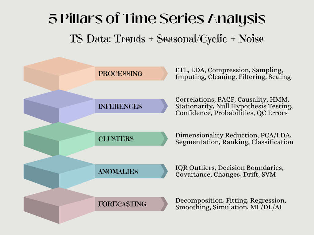
- Time Series Analysis
- Train/Test Splitting
- Random Walk Model
- Holt-Winters Model
- SARIMAX Model
- GARCH Model
- LSTM Model
- Prophet Model
- Di Pietro’s Model
- Conclusions
- References
- Explore More
- Appendix
Input Data
- Let’s set the working directory YOURPATH
import os
os.chdir('YOURPATH')
os. getcwd()
- Importing the key libraries and utility functions from Appendix
import warnings
import pandas as pd
warnings.filterwarnings("ignore")
from ts_utils6 import * # See Appendix
import pyts
- Reading the input dataset
dtf = pd.read_csv('data_sales.csv')
dtf.head()

date	date_block_num	shop_id	item_id	item_price	item_cnt_day
0	02.01.2013	0	59	22154	999.00	1.0
1	03.01.2013	0	25	2552	899.00	1.0
2	05.01.2013	0	25	2552	899.00	-1.0
3	06.01.2013	0	25	2554	1709.05	1.0
4	15.01.2013	0	25	2555	1099.00	1.0
- Grouping the data by date after datetime format conversion
dtf["date"] = pd.to_datetime(dtf['date'], format='%d.%m.%Y')
ts = dtf.groupby("date")["item_cnt_day"].sum().rename("sales")
ts.tail()date
2015-10-27    1551.0
2015-10-28    3593.0
2015-10-29    1589.0
2015-10-30    2274.0
2015-10-31    3104.0
Name: sales, dtype: float64
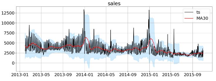
- Printing the descriptive population and 1-month moving statistics
print("population --> len:", len(ts), "| mean:", round(ts.mean()), " | std:", round(ts.std()))
w = 30
print("moving --> len:", w, " | mean:", round(ts.ewm(span=w).mean()[-1]), " | std:", round(ts.ewm(span=w).std()[-1]))

population --> len: 1034 | mean: 3528  | std: 1585
moving --> len: 30  | mean: 2305  | std: 773
Time Series Analysis
- Plotting time series (ts) sales data vs MA30
import matplotlib.pyplot as plt
plt.rcParams.update({'font.size': 18})
plot_ts(ts, plot_ma=True, plot_intervals=True, window=w, figsize=(15,5))
- Fitting the linear trend line
trend, line = fit_trend(ts, degree=1, plot=True, figsize=(15,5))
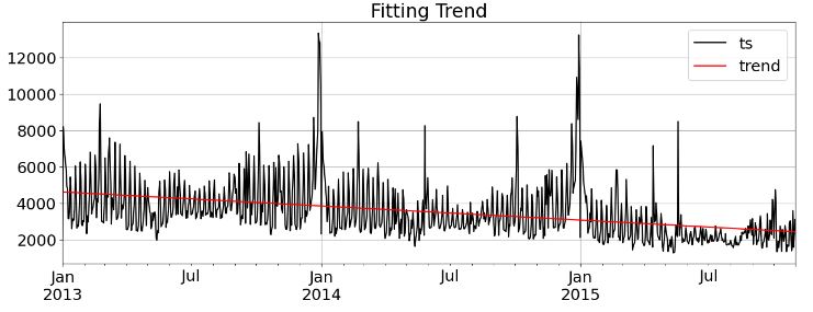
There is a slight trend and it’s linear (“additive”)
print(“constant:”, round(line[-1],2), “| slope:”, round(line[0],2))
constant: 4622.02 | slope: -2.12
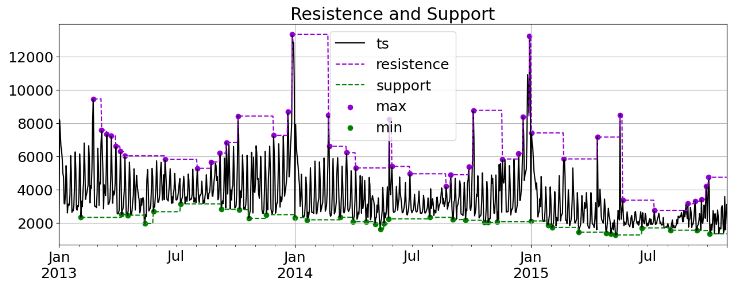
- Plotting the 1-month moving resistance/support lines with local min/max values
res_sup = resistence_support(ts, window=30, trend=False, plot=True, figsize=(15,5))
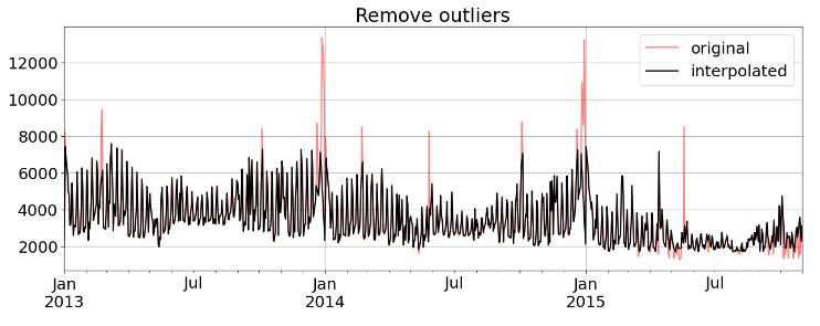
- Detecting outliers
dtf_outliers = find_outliers(ts, perc=0.05, figsize=(15,5))

- Removing outliers
ts_clean = remove_outliers(ts, outliers_idx=dtf_outliers[dtf_outliers["outlier"]==1].index, figsize=(15,5))
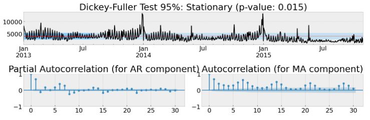
- Testing stationarity of the original data ts
test_stationarity_acf_pacf(ts, sample=0.20, maxlag=w, figsize=(15,5))
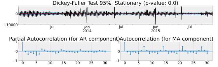
- Testing stationarity of the first-order differences
test_stationarity_acf_pacf(diff_ts(ts, order=1), sample=0.20, maxlag=30, figsize=(15,5))
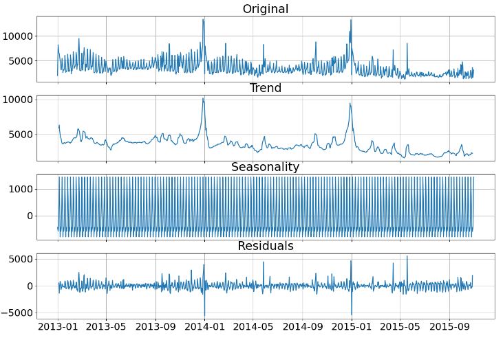
- Performing weekly seasonality & trend decomposition
dic_decomposed = decompose_ts(ts, s=7, figsize=(15,10))
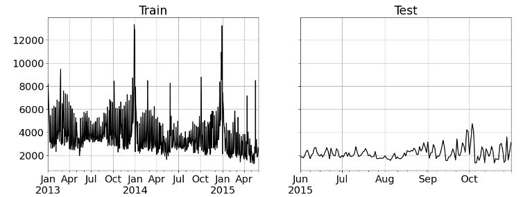
Train/Test Splitting
- Train/test data splitting
ts_train, ts_test = split_train_test(ts, exog=None, test="2015-06-01", plot=True, figsize=(15,5))
print("train:", len(ts_train), "obs  |  test:", len(ts_test), "obs")

--- splitting at index:  881 | 2015-06-01 00:00:00 | test size: 0.15  ---
train: 881 obs  |  test: 153 obs
Random Walk Model
- Implementing the Random Walk model
dtf = simulate_rw(ts_train, ts_test, conf=0.10, figsize=(15,10))
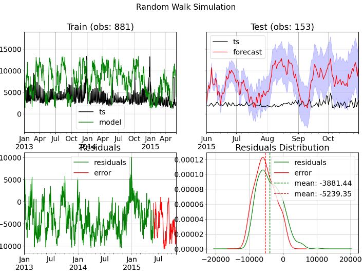
Training --> Residuals mean: -3881.0  | std: 3535.0
Test --> Error mean: -5239.0  | std: 2955.0  | mae: 5271.0  | mape: 255.0 %  | mse: 36123903.0  | rmse: 6010.0
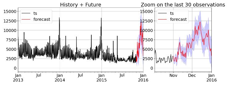
- Generating the future forecast using the Random Walk model
future = forecast_rw(ts, end="2016-01-01", conf=0.10, zoom=30, figsize=(15,5))
--- generating index date --> freq: D | start: 2015-11-01 00:00:00 | end: 2016-01-01 00:00:00 | len: 62 ---
--- computing confidence interval ---
Holt-Winters Model
- Implementing the Exponential Smoothing Model (ESM) with tuning
res = tune_expsmooth_model(ts_train, s=s, val_size=0.2, scoring=metrics.mean_absolute_error, top=4, figsize=(15,5))
res.head()
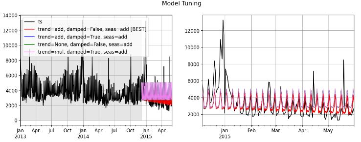
combo	score	model
0	trend=add, damped=False, seas=add	1048.356846	<statsmodels.tsa.holtwinters.results.HoltWinte...
1	trend=add, damped=True, seas=add	1301.840904	<statsmodels.tsa.holtwinters.results.HoltWinte...
2	trend=None, damped=False, seas=add	1309.152958	<statsmodels.tsa.holtwinters.results.HoltWinte...
3	trend=mul, damped=True, seas=add	1319.483026	<statsmodels.tsa.holtwinters.results.HoltWinte...
4	trend=add, damped=True, seas=None	1483.018551	<statsmodels.tsa.holtwinters.results.HoltWinte...
- Implementing the ESM multiplicative seasonality every 6 observations
dtf, model = fit_expsmooth(ts_train, ts_test, trend="additive", damped=False, seasonal="multiplicative", s=6,
                           factors=(None,None,None), conf=0.10, figsize=(15,10)

Seasonal parameters: multiplicative Seasonality every 6 observations
--- computing confidence interval ---
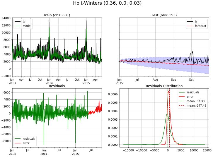
Training --> Residuals mean: 32.0  | std: 1413.0
Test --> Error mean: 647.0  | std: 748.0  | mae: 696.0  | mape: 28.0 %  | mse: 974519.0  | rmse: 987.0
It seems that the average error of prediction is in 388 unit of sales (16% of the predicted value).
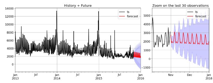
- Generating the future forecast using the ESM model
model = smt.ExponentialSmoothing(ts, trend="additive", damped=False,
                                 seasonal="multiplicative", seasonal_periods=s).fit(0.64)

future = forecast_autoregressive(ts, model, end="2016-01-01", conf=0.30, zoom=30, figsize=(15,5))

--- generating index date --> freq: D | start: 2015-11-01 00:00:00 | end: 2016-01-01 00:00:00 | len: 62 ---
--- computing confidence interval ---
SARIMAX Model
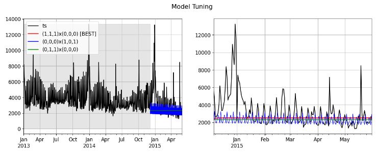
- Tuning the SARIMAX model
res = tune_arima_model(ts_train, s=s, val_size=0.2, max_order=(1,1,1), seasonal_order=(1,0,1),
                        scoring=metrics.mean_absolute_error, top=3, figsize=(15,5))
res.head()
combo	score	model
0	(1,1,1)x(0,0,0)	1267.729997	<statsmodels.tsa.statespace.sarimax.SARIMAXRes...
1	(0,0,0)x(1,0,1)	1284.688508	<statsmodels.tsa.statespace.sarimax.SARIMAXRes...
2	(0,1,1)x(0,0,0)	1288.717213	<statsmodels.tsa.statespace.sarimax.SARIMAXRes...
3	(1,1,0)x(0,0,0)	1293.258417	<statsmodels.tsa.statespace.sarimax.SARIMAXRes...
4	(0,1,0)x(0,0,0)	1296.548023	<statsmodels.tsa.statespace.sarimax.SARIMAXRes...
- Finding the best SARIMAX model
find_best_sarimax(ts_train, seasonal=True, stationary=False, s=s, exog=None,
max_p=10, max_d=3, max_q=10,
max_P=1, max_D=1, max_Q=1)
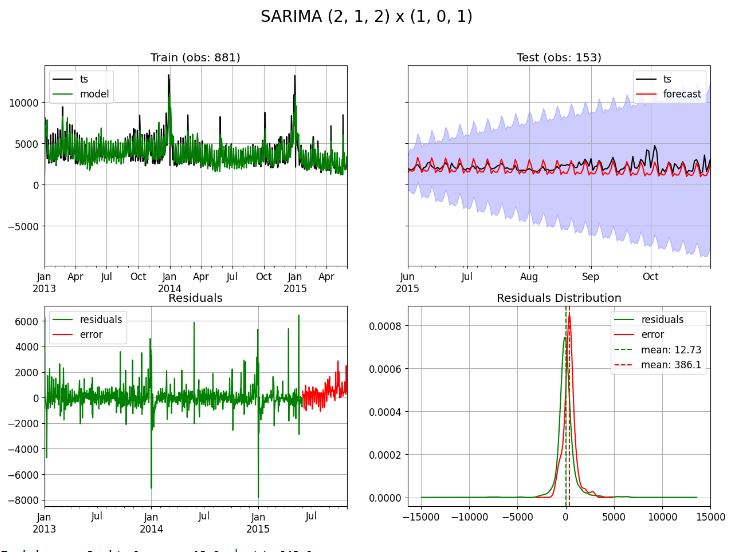
best model --> (p, d, q): (2, 1, 2) and (P, D, Q, s): (1, 0, 1, 7)
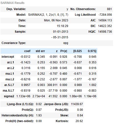
- Fitting with the best SARIMAX model
dtf, model = fit_sarimax(ts_train, ts_test, order=(2,1,2), seasonal_order=(1, 0, 1), s=s, conf=0.95, figsize=(15,10))

Trend parameters: d=1
Seasonal parameters: Seasonality every 7 observations
Exog parameters: Not given

Training --> Residuals mean: 13.0  | std: 948.0
Test --> Error mean: 386.0  | std: 644.0  | mae: 567.0  | mape: 24.0 %  | mse: 560661.0  | rmse: 749.0
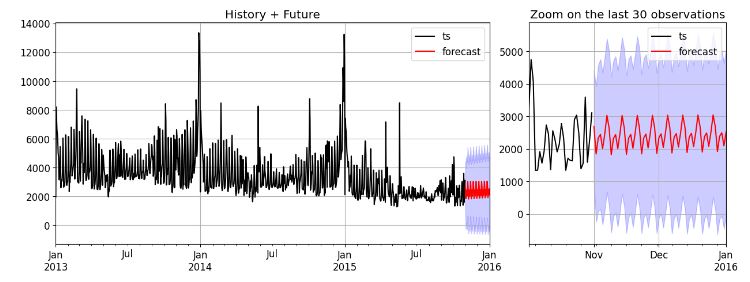
- Forecast with the best SARIMAX model
model = smt.SARIMAX(ts, order=(2,1,2), seasonal_order=(1,0,1,s), exog=None).fit()

future = forecast_autoregressive(ts, model, end="2016-01-01", conf=0.95, zoom=30, figsize=(15,5))

--- generating index date --> freq: D | start: 2015-11-01 00:00:00 | end: 2016-01-01 00:00:00 | len: 62 ---
GARCH Model
- Implementing the GARCH model
fit_garch(ts_train, ts_test, order=(2,1,2), seasonal_order=(1,0,1,s), figsize=(15,10))
Iteration:      7,   Func. Count:     70,   Neg. LLF: 7732.775377088017
Iteration:     14,   Func. Count:    139,   Neg. LLF: 6935.63535033199
Iteration:     21,   Func. Count:    202,   Neg. LLF: 6931.972089490232
Iteration:     28,   Func. Count:    265,   Neg. LLF: 6929.40082625206
Optimization terminated successfully    (Exit mode 0)
            Current function value: 6929.400098515533
            Iterations: 32
            Function evaluations: 300
            Gradient evaluations: 32
--- got error ---
unsupported operand type(s) for -: 'float' and 'ARCHModelForecast'
(None,
                       Constant Mean - GJR-GARCH Model Results
 ====================================================================================
 Dep. Variable:                         None   R-squared:                       0.000
 Mean Model:                   Constant Mean   Adj. R-squared:                  0.000
 Vol Model:                        GJR-GARCH   Log-Likelihood:               -6929.40
 Distribution:      Standardized Student's t   AIC:                           13874.8
 Method:                  Maximum Likelihood   BIC:                           13913.0
                                               No. Observations:                  881
 Date:                      Mon, Nov 06 2023   Df Residuals:                      880
 Time:                              15:36:09   Df Model:                            1
                                Mean Model
 ========================================================================
                  coef    std err          t      P>|t|  95.0% Conf. Int.
 ------------------------------------------------------------------------
 mu           -46.3875     17.871     -2.596  9.440e-03 [-81.414,-11.361]
                               Volatility Model
 ============================================================================
                  coef    std err          t      P>|t|      95.0% Conf. Int.
 ----------------------------------------------------------------------------
 omega      2.6917e+05  9.054e+04      2.973  2.950e-03 [9.171e+04,4.466e+05]
 alpha[1]       0.4922      0.216      2.274  2.294e-02   [6.806e-02,  0.916]
 alpha[2]       0.3848      0.267      1.442      0.149     [ -0.138,  0.908]
 gamma[1]      -0.2185      0.230     -0.949      0.343     [ -0.670,  0.233]
 beta[1]        0.1428      0.231      0.618      0.536     [ -0.310,  0.595]
 beta[2]        0.0000  5.892e-02      0.000      1.000     [ -0.115,  0.115]
                               Distribution
 ========================================================================
                  coef    std err          t      P>|t|  95.0% Conf. Int.
 ------------------------------------------------------------------------
 nu             2.7612      0.187     14.790  1.700e-49 [  2.395,  3.127]
 ========================================================================

 Covariance estimator: robust
 ARCHModelResult, id: 0x2412979da00)
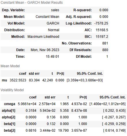
- Fitting the GARCH model
import arch
from arch import arch_model
model = arch_model(ts_train, p=2, q=2)
model_fit = model.fit()
model_fit.summary()

Iteration:      1,   Func. Count:      8,   Neg. LLF: 8625.687094584897
Iteration:      2,   Func. Count:     16,   Neg. LLF: 7591.663085839065
Iteration:      3,   Func. Count:     23,   Neg. LLF: 7590.181494531133
Iteration:      4,   Func. Count:     30,   Neg. LLF: 7589.836295096868
Iteration:      5,   Func. Count:     37,   Neg. LLF: 7589.827769095689
Iteration:      6,   Func. Count:     44,   Neg. LLF: 7589.806877638113
Iteration:      7,   Func. Count:     51,   Neg. LLF: 7589.782971327825
Iteration:      8,   Func. Count:     58,   Neg. LLF: 7589.697896589118
Iteration:      9,   Func. Count:     65,   Neg. LLF: 7589.475629047222
Iteration:     10,   Func. Count:     72,   Neg. LLF: 7588.901641267379
Iteration:     11,   Func. Count:     79,   Neg. LLF: 7587.335035285622
Iteration:     12,   Func. Count:     86,   Neg. LLF: 7583.837150680619
Iteration:     13,   Func. Count:     93,   Neg. LLF: 7579.646854205145
Iteration:     14,   Func. Count:    100,   Neg. LLF: 7578.593139426219
Iteration:     15,   Func. Count:    107,   Neg. LLF: 7578.292100471091
Iteration:     16,   Func. Count:    114,   Neg. LLF: 7578.255669462309
Iteration:     17,   Func. Count:    121,   Neg. LLF: 7578.2502424651775
Iteration:     18,   Func. Count:    128,   Neg. LLF: 7578.245473206713
Iteration:     19,   Func. Count:    135,   Neg. LLF: 7583.610036013718
Iteration:     20,   Func. Count:    145,   Neg. LLF: 7578.245736636854
Iteration:     21,   Func. Count:    154,   Neg. LLF: 7578.245736770681
Iteration:     22,   Func. Count:    160,   Neg. LLF: 7578.24573671558
Optimization terminated successfully    (Exit mode 0)
            Current function value: 7578.245736770681
            Iterations: 23
            Function evaluations: 160
            Gradient evaluations: 22
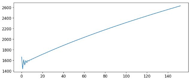
- GARCH predictions with horizon=153 which is len(ts_test)
predictions = model_fit.forecast(horizon=153)
plt.figure(figsize=(10,4))
preds, = plt.plot(np.sqrt(predictions.variance.values[-1, :]))
LSTM Model
- Implementing the LSTM Sequential model
s = 130
n_features = 1
model = models.Sequential()
model.add( layers.LSTM(input_shape=(s,n_features), units=50, activation='relu', return_sequences=True) )
model.add( layers.Dropout(0.2) )
model.add( layers.LSTM(units=50, activation='relu', return_sequences=False) )
model.add( layers.Dense(1) )
model.compile(optimizer='adam', loss='mean_absolute_error')
model.summary()
Model: "sequential_1"
_________________________________________________________________
Layer (type) Output Shape Param #
=================================================================
lstm_2 (LSTM) (None, 130, 50) 10400
dropout_1 (Dropout) (None, 130, 50) 0
lstm_3 (LSTM) (None, 50) 20200
dense_1 (Dense) (None, 1) 51
=================================================================
Total params: 30,651
Trainable params: 30,651
Non-trainable params: 0
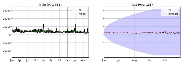
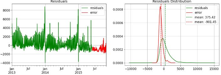
dtf, model = fit_lstm(ts_train, ts_test, model, exog=None, s=s, epochs=1, conf=0.30, figsize=(15,10))
Training --> Residuals mean: 375.0 | std: 1451.0
Test --> Error mean: -901.0 | std: 559.0 | mae: 976.0 | mape: 50.0 % | mse: 1123190.0 | rmse: 1060.0
- LSTM (memory: 130) forecasting
Prophet Model
- Implementing the Prophet model
dtf_train = ts_train.reset_index().rename(columns={"date":"ds", "sales":"y"})
dtf_test = ts_test.reset_index().rename(columns={"date":"ds", "sales":"y"})
dtf_train.tail()
ds y
876 2015-05-27 1953.0
877 2015-05-28 1885.0
878 2015-05-29 2146.0
879 2015-05-30 2665.0
880 2015-05-31 2283.0
dtf_holidays = None
from prophet.forecaster import Prophet
model = Prophet(growth="linear", changepoints=None, n_changepoints=25, seasonality_mode="multiplicative",
yearly_seasonality="auto", weekly_seasonality="auto", daily_seasonality=False,
holidays=dtf_holidays, interval_width=0.80)
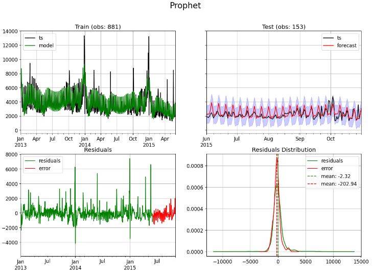
dtf, model = fit_prophet(dtf_train, dtf_test, model=model, figsize=(15,10))
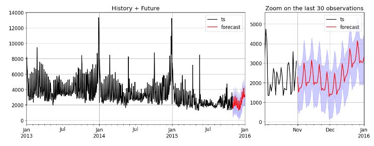
future = forecast_prophet(dtf, model, end="2016-01-01", zoom=30, figsize=(15,5))
Training --> Residuals mean: -2.0 | std: 962.0
Test --> Error mean: -203.0 | std: 573.0 | mae: 448.0 | mape: 20.0 % | mse: 367888.0 | rmse: 607.0
Di Pietro’s Model
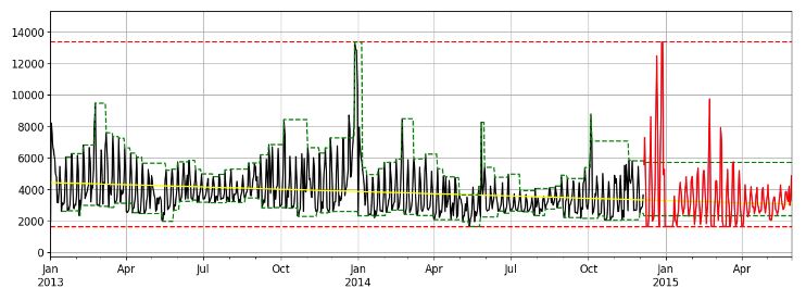
- Tuning the custom model
# Tuning
tune = custom_model(ts_train.head(int(0.8*len(ts_train))), pred_ahead=int(0.2*len(ts_train)),
                    trend=True, seasonality_types=["dow","dom","doy","woy","moy"],
                    level_window=7, sup_res_windows=(365,365), floor_cap=(True,True),
                    plot=True, figsize=(15,5))

--- generating index date --> freq: D | start: 2014-12-06 00:00:00 | end: 2015-05-30 00:00:00 | len: 176 ---
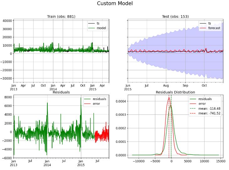
- Fitting the custom model
trend = True
seasonality_types = ["dow","dom","doy","woy","moy"]
level_window = 7
sup_res_windows = (365,365)
floor_cap = (True,True)

dtf = fit_custom_model(ts_train, ts_test, trend, seasonality_types, level_window, sup_res_windows, floor_cap,
                       conf=0.1, figsize=(15,10))

--- generating index date --> freq: D | start: 2015-06-01 00:00:00 | end: 2015-10-31 00:00:00 | len: 153 ---
--- computing confidence interval ---

Training --> Residuals mean: -116.0  | std: 1398.0
Test --> Error mean: -742.0  | std: 851.0  | mae: 930.0  | mape: 44.0 %  | mse: 1269838.0  | rmse: 1127.0
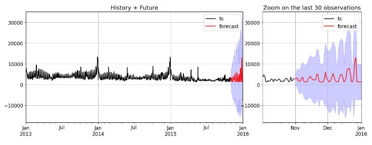
- Custom model future forecasting
future = forecast_custom_model(ts, trend, seasonality_types, level_window, sup_res_windows, floor_cap,
                               conf=0.3, end="2016-01-01", zoom=30, figsize=(15,5))

--- generating index date --> freq: D | start: 2015-11-01 00:00:00 | end: 2016-01-01 00:00:00 | len: 62 ---
--- generating index date --> freq: D | start: 2015-11-01 00:00:00 | end: 2016-01-01 00:00:00 | len: 62 ---
--- computing confidence interval ---
Conclusions
- We have evaluated several ML-type time series analysis (TSA) algorithms to analyze historical sales data and make predictions about future sales.
- TSA involves analyzing data collected over time, such as sales data, and modeling historical trends and seasonal patterns to make predictions about the future.
- TSA s useful for predicting sales because it takes into account historical patterns and trends, such as seasonality and long-term trends, to make accurate predictions.
- The technique can also identify anomalies or unexpected events that may impact future sales, allowing businesses to make necessary adjustments to their strategy.
- In this case study, tslearn, Random Walk and GARCH did not performed well on the training and test sets.
- We summarize the key performance metrics of other 5 models in Table below:
| Methods/Scores | RMSE | STD | MAPE % |
| Prophet | 607 | 573 | 20 |
| LSTM | 1060 | 559 | 50 |
| SARIMAX | 749 | 644 | 24 |
| HW | 987 | 748 | 28 |
| Custom | 1127 | 851 | 44 |
- It appears that the 3 best performing models are Prophet, SARIMAX, and Holt-Winters.
- These models use TSA to generate most accurate future sales based on historical train data. Traditional methods, on the other hand, can be time-intensive, error-prone, and vulnerable to human biases.
- Our results enable businesses to swiftly generate accurate forecasts, monitor market trends, and make data-driven decisions.
References
- Predict Future Sales
- DataScience_ArtificialIntelligence_Utils
- Time Series Analysis for Machine Learning
- Time Series Forecasting with Random Walk
- Time Series Forecasting: ARIMA vs LSTM vs PROPHET
Explore More
- A Balanced Mix-and-Match Time Series Forecasting: ThymeBoost, Prophet, and AutoARIMA
- Predicting Rolling Volatility of the NVIDIA Stock – GARCH vs XGBoost
- Time Series Forecasting of Hourly U.S.A. Energy Consumption – PJM East Electricity Grid
- Risk-Return Analysis and LSTM Price Predictions of 4 Major Tech Stocks in 2023
- SARIMAX X-Validation of EIA Crude Oil Prices Forecast in 2023 – 1. WTI
- BTC-USD Freefall vs FB/Meta Prophet 2022-23 Predictions
- BTC-USD Price Prediction with LSTM
- SARIMAX-TSA Forecasting, QC and Visualization of Online Food Delivery Sales
- Stock Forecasting with FBProphet
- Predicting the JPM Stock Price and Breakouts with Auto ARIMA, FFT, LSTM and Technical Trading Indicators
- S&P 500 Algorithmic Trading with FBProphet
Appendix


One-Time
Monthly
Yearly
Make a one-time donation
Make a monthly donation
Make a yearly donation
Choose an amount
€5.00
€15.00
€100.00
€5.00
€15.00
€100.00
€5.00
€15.00
€100.00
Or enter a custom amount
€
Your contribution is appreciated.
Your contribution is appreciated.
Your contribution is appreciated.

Leave a comment