
- It is no secret that AI carries enormous transformational potential for industries and society. Within the insurance sector, insurers are already using AI to improve customer service, to increase efficiency and to fight against fraud more effectively.
- Cross-sell is the selling of additional products or services to existing customers. This type of sale involves an implementation that can increase customer longevity and reduce churn.
- In this walkthrough, we will discuss best industry practices of insurance price predictions by combining Machine Learning (ML) with model tuning (aka hyperparameter optimization).
- Predicting the medical insurance cost is very important task in healthtech. As insurance providers strive to offer competitive and personalized healthcare plans, it becomes essential to understand the factors influencing premium prices and create models that can accurately predict them.
- Scope: input data preparation, Exploratory Data Analysis (EDA), Feature Engineering (FE), ML models training, testing and cross-validation, parameter optimization, and final classification report with relevant QC metrics.
- About dataset: The client is an Insurance company that has provided Health Insurance to its customers. Now they need AI help in building a model to predict whether the policyholders (customers) from past year will also be interested in Vehicle Insurance provided by the company.
- Read more here.
Table of Contents
- ML Tuning Pipelines
- HGBM Model Tuning, Validation & Interpretation
- XGB Model Validation
- IQR Filtering & RF Modeling
- Conclusions
- References
- Explore More
ML Tuning Pipelines
- Setting the working directory YOURPATH
import os
os.chdir('YOURPATH')
os. getcwd()
- Reading the input dataset and looking at the basic structure
import numpy as np # linear algebra
import pandas as pd # data processing, CSV file I/O (e.g. pd.read_csv)

df = pd.read_csv('train.csv')

#Descriptive statistics of continuous variables
df.describe().T

df.describe(include=object).T

count	         unique	    top	        freq
Gender	        381109	2	Male	    206089
Vehicle_Age	    381109	3	1-2 Year	200316
Vehicle_Damage	381109	2	Yes	        192413
- Check for possible nulls in the dataset
df.isnull().sum()
id                      0
Gender                  0
Age                     0
Driving_License         0
Region_Code             0
Previously_Insured      0
Vehicle_Age             0
Vehicle_Damage          0
Annual_Premium          0
Policy_Sales_Channel    0
Vintage                 0
Response                0
dtype: int64

# Categorical variables
for i in df.select_dtypes(include=['object']).columns:
    print(df[i].value_counts())

Male      206089
Female    175020
Name: Gender, dtype: int64
1-2 Year     200316
< 1 Year     164786
> 2 Years     16007
Name: Vehicle_Age, dtype: int64
Yes    192413
No     188696
Name: Vehicle_Damage, dtype: int64
- Data preparation
df_trimmed = df.loc[:,['Gender','Age','Driving_License','Previously_Insured','Vehicle_Age','Vehicle_Damage','Annual_Premium','Vintage','Response']]
#Drop null values and create dummy variables
df_final = pd.get_dummies(df_trimmed).dropna()

df_final.columns
Index(['Age', 'Driving_License', 'Previously_Insured', 'Annual_Premium',
       'Vintage', 'Response', 'Gender_Female', 'Gender_Male',
       'Vehicle_Age_1-2 Year', 'Vehicle_Age_< 1 Year', 'Vehicle_Age_> 2 Years',
       'Vehicle_Damage_No', 'Vehicle_Damage_Yes'],
      dtype='object')

df_final.Response.value_counts()
0    334399
1     46710
Name: Response, dtype: int64
- Train/test split with test_size=0.2 and SMOTE resampling
#Create train test split

from sklearn.model_selection import train_test_split
X = df_final.drop('Response', axis =1)
y = df_final.loc[:,['Response']]

X_train, X_test, y_train, y_test = train_test_split(X, y, test_size=0.2, random_state=42)

#balance the data (SMOTE)
from imblearn.over_sampling import SMOTE
smote = SMOTE(sampling_strategy =1)

X_train, y_train = smote.fit_resample(X_train,y_train)
- Create the baseline ML model using the Naïve Bayes algorithm
from sklearn.model_selection import cross_val_score

#import Naive Bayes Classifier
from sklearn.naive_bayes import GaussianNB

#create classifier object
nb = GaussianNB()

#run cv for NB classifier
from sklearn.metrics import classification_report

nb_accuracy = cross_val_score(nb,X_train,y_train.values.ravel(), cv=3, scoring ='accuracy')
nb_f1 = cross_val_score(nb,X_train,y_train.values.ravel(), cv=3, scoring ='f1')

print('nb_accuracy: ' +str(nb_accuracy))
print('nb F1_Macro Score: '+str(nb_f1))
print('nb_accuracy_avg: ' + str(nb_accuracy.mean()) +'  |  lr_f1_avg: '+str(nb_f1.mean()))

nb_accuracy: [0.80302801 0.81294581 0.81078189]
nb F1_Macro Score: [0.82865318 0.83993805 0.83826875]
nb_accuracy_avg: 0.8089185690386936  |  lr_f1_avg: 0.8356199930577949
- Comparison with other ML algorithms
#Model Comparison & Selection

## Decision Tree
from sklearn.tree import DecisionTreeClassifier
dt = DecisionTreeClassifier(random_state =32)

dt_accuracy = cross_val_score(dt,X_train,y_train.values.ravel(), cv=3, scoring ='accuracy')
dt_f1 = cross_val_score(dt,X_train,y_train.values.ravel(), cv=3, scoring ='f1')

print('dt_accuracy: ' +str(dt_accuracy))
print('dt F1_Macro Score: '+str(dt_f1))
print('dt_accuracy_avg: ' + str(dt_accuracy.mean()) +'  |  dt_f1_avg: '+str(dt_f1.mean())+'\n')


## Logistic Regression
from sklearn.linear_model import LogisticRegression
lr = LogisticRegression(random_state=32, max_iter = 2000, class_weight = 'balanced')

lr_accuracy = cross_val_score(lr,X_train,y_train.values.ravel(), cv=3, scoring ='accuracy')
lr_f1 = cross_val_score(lr,X_train,y_train.values.ravel(), cv=3, scoring ='f1')

print('lr_accuracy: ' +str(lr_accuracy))
print('lr F1_Macro Score: '+str(lr_f1))
print('lr_accuracy_avg: ' + str(lr_accuracy.mean()) +'  |  lr_f1_avg: '+str(lr_f1.mean())+'\n')


## KNN
from sklearn.neighbors import KNeighborsClassifier
from sklearn.preprocessing import StandardScaler
from sklearn.pipeline import make_pipeline, Pipeline

knn = make_pipeline(StandardScaler(), KNeighborsClassifier(n_neighbors=3))
knn_accuracy = cross_val_score(knn,X_train,y_train.values.ravel(), cv=3, scoring ='accuracy')
knn_f1 = cross_val_score(knn,X_train,y_train.values.ravel(), cv=3, scoring ='f1')

print('knn_accuracy: ' +str(knn_accuracy))
print('knn F1_Macro Score: '+str(knn_f1))
print('knn_accuracy_avg: ' + str(knn_accuracy.mean()) +'  |  knn_f1_avg: '+str(knn_f1.mean()))

dt_accuracy: [0.82508811 0.8866345  0.8839835 ]
dt F1_Macro Score: [0.81301514 0.89198078 0.88957392]
dt_accuracy_avg: 0.8652353730820522  |  dt_f1_avg: 0.8648566148576409

lr_accuracy: [0.79171499 0.8250713  0.56066141]
lr F1_Macro Score: [0.80549422 0.84384176 0.60709078]
lr_accuracy_avg: 0.7258159037084625  |  lr_f1_avg: 0.752142250293187

knn_accuracy: [0.80213149 0.87422325 0.87273766]
knn F1_Macro Score: [0.78854111 0.88014651 0.87883444]
knn_accuracy_avg: 0.849697465521477  |  knn_f1_avg: 0.8491740207579683
- Let’s optimize the KNN model by changing the K-parameter
#Manual Parameter Tuning
#Here we will loop through and see which value of k performs the best.

for i in range(1,7):
    knn = make_pipeline(StandardScaler(), KNeighborsClassifier(n_neighbors=i))
    knn_f1 = cross_val_score(knn,X_train,y_train.values.ravel(), cv=3, scoring ='f1')
    print('K ='+(str(i)) + (': ') + str(knn_f1.mean()))

K =1: 0.8419050988542729
K =2: 0.8177949676361784
K =3: 0.8491740207579683
K =4: 0.8352706032017148
K =5: 0.8504233464794012
K =6: 0.8405313324705315
- Implementing the Decision Tree model tuning using RandomizedSearchCV
#Randomized Parameter Tuning

from sklearn.model_selection import RandomizedSearchCV

dt = DecisionTreeClassifier(random_state = 42)

features = {'criterion': ['gini','entropy'],
            'splitter': ['best','random'],
           'max_depth': [2,5,10,20,40,None],
           'min_samples_split': [2,5,10,15],
           'max_features': ['auto','sqrt','log2',None]}

rs_dt = RandomizedSearchCV(estimator = dt, param_distributions =features, n_iter =100, cv = 3, random_state = 42, scoring ='f1')

rs_dt.fit(X_train,y_train)

RandomizedSearchCV(cv=3, estimator=DecisionTreeClassifier(random_state=42),
                   n_iter=100,
                   param_distributions={'criterion': ['gini', 'entropy'],
                                        'max_depth': [2, 5, 10, 20, 40, None],
                                        'max_features': ['auto', 'sqrt', 'log2',
                                                         None],
                                        'min_samples_split': [2, 5, 10, 15],
                                        'splitter': ['best', 'random']},
                   random_state=42, scoring='f1')

print('best stcore = ' + str(rs_dt.best_score_))
print('best params = ' + str(rs_dt.best_params_))

best stcore = 0.8628995334929804
best params = {'splitter': 'best', 'min_samples_split': 2, 'max_features': None, 'max_depth': 40, 'criterion': 'gini'}
- Implementing the Decision Tree model tuning using GridSearchCV
#GridsearchCV (Exhaustive Parameter Tuning)
from sklearn.model_selection import GridSearchCV


features_gs = {'criterion': ['entropy'],
            'splitter': ['random'],
           'max_depth': np.arange(30,50,1), #getting more precise within range
           'min_samples_split': [2,3,4,5,6,7,8,9],
           'max_features': [None]}

gs_dt = GridSearchCV(estimator = dt, param_grid =features_gs, cv = 3, scoring ='f1') #we don't need random state because there isn't randomization like before

gs_dt.fit(X_train,y_train)

GridSearchCV(cv=3, estimator=DecisionTreeClassifier(random_state=42),
             param_grid={'criterion': ['entropy'],
                         'max_depth': array([30, 31, 32, 33, 34, 35, 36, 37, 38, 39, 40, 41, 42, 43, 44, 45, 46,
       47, 48, 49]),
                         'max_features': [None],
                         'min_samples_split': [2, 3, 4, 5, 6, 7, 8, 9],
                         'splitter': ['random']},
             scoring='f1')

print('best stcore = ' + str(gs_dt.best_score_))
print('best params = ' + str(gs_dt.best_params_))

best stcore = 0.848931249858977
best params = {'criterion': 'entropy', 'max_depth': 31, 'max_features': None, 'min_samples_split': 2, 'splitter': 'random'}
- Implementing the Decision Tree model tuning using BayesSearchCV
#Bayesian Optimization
from skopt import BayesSearchCV
from sklearn.model_selection import StratifiedKFold
from skopt import BayesSearchCV
from skopt.space import Real, Categorical, Integer

# Choose cross validation method
cv = StratifiedKFold(n_splits = 3)


bs_lr = BayesSearchCV(
    dt,
    {'criterion': Categorical(['gini','entropy']),
            'splitter': Categorical(['best','random']),
           'max_depth': Integer(10,50),
           'min_samples_split': Integer(2,15),
           'max_features': Categorical(['sqrt','log2',None])},
    random_state=42,
    n_iter= 100,
    cv= cv,
    scoring ='f1')

bs_lr.fit(X_train,y_train.values.ravel())

BayesSearchCV(cv=StratifiedKFold(n_splits=3, random_state=None, shuffle=False),
              estimator=DecisionTreeClassifier(random_state=42), n_iter=100,
              random_state=42, scoring='f1',
              search_spaces={'criterion': Categorical(categories=('gini', 'entropy'), prior=None),
                             'max_depth': Integer(low=10, high=50, prior='uniform', transform='normalize'),
                             'max_features': Categorical(categories=('sqrt', 'log2', None), prior=None),
                             'min_samples_split': Integer(low=2, high=15, prior='uniform', transform='normalize'),
                             'splitter': Categorical(categories=('best', 'random'), prior=None)})

print('best stcore = ' + str(bs_lr.best_score_))
print('best params = ' + str(bs_lr.best_params_))

best stcore = 0.8646572554143731
best params = OrderedDict([('criterion', 'entropy'), ('max_depth', 50), ('max_features', None), ('min_samples_split', 2), ('splitter', 'best')])
- Implementing the Voting Classifier by optimizing the Logistic Regression, Decision Tree, and KNN models within the following pipeline
from sklearn.ensemble import VotingClassifier

dt_voting = DecisionTreeClassifier(**{'criterion': 'entropy', 'max_depth': 50, 'max_features': None, 'min_samples_split': 2, 'splitter': 'best'}) # ** allows you to pass in parameters as dict
knn_voting = make_pipeline(StandardScaler(), KNeighborsClassifier(n_neighbors=5))
lr_voting = LogisticRegression(random_state=32, max_iter = 2000, class_weight = 'balanced')

ens = VotingClassifier(estimators = [('dt', dt_voting), ('knn', knn_voting), ('lr',lr_voting)], voting = 'hard')

voting_accuracy = cross_val_score(ens,X_train,y_train.values.ravel(), cv=3, scoring ='accuracy')
voting_f1 = cross_val_score(ens,X_train,y_train.values.ravel(), cv=3, scoring ='f1')

print('voting_accuracy: ' +str(voting_accuracy))
print('voting F1_Macro Score: '+str(voting_f1))
print('voting_accuracy_avg: ' + str(voting_accuracy.mean()) +'  |  voting_f1_avg: '+str(voting_f1.mean()))

voting_accuracy: [0.82490881 0.87750116 0.87486692]
voting F1_Macro Score: [0.82273785 0.88742814 0.88349019]
voting_accuracy_avg: 0.8590922969268296  |  voting_f1_avg: 0.8645520579723294

ens = VotingClassifier(estimators = [('dt', dt_voting), ('knn', knn_voting), ('lr',lr_voting)], voting = 'soft')
voting_accuracy = cross_val_score(ens,X_train,y_train.values.ravel(), cv=3, scoring ='accuracy')
voting_f1 = cross_val_score(ens,X_train,y_train.values.ravel(), cv=3, scoring ='f1')

print('voting_accuracy: ' +str(voting_accuracy))
print('voting F1_Macro Score: '+str(voting_f1))
print('voting_accuracy_avg: ' + str(voting_accuracy.mean()) +'  |  voting_f1_avg: '+str(voting_f1.mean()))

voting_accuracy: [0.82665703 0.88745258 0.88575415]
voting F1_Macro Score: [0.81886784 0.89410882 0.89215842]
voting_accuracy_avg: 0.866621253516802  |  voting_f1_avg: 0.8683783597723743
- Implementing the Stacking Classifier by cascading the Logistic Regression, Decision Tree, and GaussianNB models within the following pipeline
#Stacking Classifier
from sklearn.ensemble import StackingClassifier

ens_stack = StackingClassifier(estimators = [('dt', dt_voting), ('lr',lr_voting), ('nb',GaussianNB())], final_estimator = GaussianNB())

stack_accuracy = cross_val_score(ens_stack,X_train,y_train.values.ravel(), cv=3, scoring ='accuracy')
stack_f1 = cross_val_score(ens_stack,X_train,y_train.values.ravel(), cv=3, scoring ='f1')

print('stacking_accuracy: ' +str(stack_accuracy))
print('stacking F1_Macro Score: '+str(stack_f1))
print('stacking_accuracy_avg: ' + str(stack_accuracy.mean()) +'  |  stack_f1_avg: '+str(stack_f1.mean()))

stacking_accuracy: [0.81573624 0.83978551 0.87037867]
stacking F1_Macro Score: [0.80105482 0.85657788 0.87878055]
stacking_accuracy_avg: 0.841966806895526  |  stack_f1_avg: 0.8454710837994078
- Let’s look at the Random Forest (RF) Classifier
#Ensemble Models
from sklearn.ensemble import RandomForestClassifier

#first let's try a non-tuned implementation
rf = RandomForestClassifier(random_state=42)

rf_accuracy = cross_val_score(rf,X_train,y_train.values.ravel(), cv=3, scoring ='accuracy')
rf_f1 = cross_val_score(rf,X_train,y_train.values.ravel(), cv=3, scoring ='f1')

print('rf_accuracy: ' +str(rf_accuracy))
print('rf F1_Macro Score: '+str(rf_f1))
print('rf_accuracy_avg: ' + str(rf_accuracy.mean()) +'  |  rf_f1_avg: '+str(rf_f1.mean()))

rf_accuracy: [0.81875641 0.89067447 0.88857822]
rf F1_Macro Score: [0.80563167 0.89648843 0.89457472]
rf_accuracy_avg: 0.866003030584957  |  rf_f1_avg: 0.8655649389116813
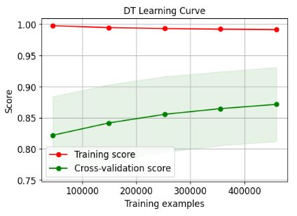
- Comparing the SciKit-Plot learning curves – Random Forest (RF) vs Decision Tree (DT)
import scikitplot as skplt

import sklearn

import matplotlib.pyplot as plt

import sys
import warnings
warnings.filterwarnings("ignore")

print("Scikit Plot Version : ", skplt.__version__)
print("Scikit Learn Version : ", sklearn.__version__)
print("Python Version : ", sys.version)

Scikit Plot Version :  0.3.7
Scikit Learn Version :  1.3.2
Python Version :  3.9.16 (main, Jan 11 2023, 16:16:36) [MSC v.1916 64 bit (AMD64)]
skplt.estimators.plot_learning_curve(rf,X_train,y_train.values.ravel(),
                                     cv=7, shuffle=True, scoring="accuracy",
                                     n_jobs=-1, figsize=(6,4), title_fontsize="large", text_fontsize="large",
                                     title="RF Learning Curve");

skplt.estimators.plot_learning_curve(dt,X_train,y_train.values.ravel(),
                                     cv=7, shuffle=True, scoring="accuracy",
                                     n_jobs=-1, figsize=(6,4), title_fontsize="large", text_fontsize="large",
                                     title="DT Learning Curve");
HGBM Model Tuning, Validation & Interpretation
- Let’s implement the HGBM model to predict insurance cross sell
import numpy as np
import pandas as pd
import matplotlib
import matplotlib.pyplot as plt
plt.style.use('ggplot')
%matplotlib inline
import seaborn as sns
import scipy
import scipy.stats as stats
import sklearn
from sklearn.model_selection import train_test_split
from sklearn.preprocessing import MinMaxScaler
from sklearn.preprocessing import StandardScaler
from sklearn.metrics import roc_auc_score
from sklearn.metrics import roc_curve, auc
from sklearn.metrics import precision_score, recall_score, f1_score
from sklearn.model_selection import StratifiedKFold
from sklearn.model_selection import GridSearchCV
from sklearn.model_selection import RandomizedSearchCV
from sklearn.linear_model import LogisticRegression
from sklearn.naive_bayes import GaussianNB
from sklearn.ensemble import HistGradientBoostingClassifier
from sklearn.cluster import KMeans
from sklearn.metrics import silhouette_score
from sklearn.calibration import CalibratedClassifierCV
from sklearn.calibration import calibration_curve
import pickle
import time
import shap


import warnings
warnings.simplefilter(action='ignore', category=UserWarning)
warnings.simplefilter(action='ignore', category=FutureWarning)

df = pd.read_csv('train.csv')

# Formatting features
df['Driving_License'] = df['Driving_License'].astype('object')
df['Region_Code'] = df['Region_Code'].astype('object')
df['Previously_Insured'] = df['Previously_Insured'].astype('object')
df['Policy_Sales_Channel'] = df['Policy_Sales_Channel'].astype('object')
df['Response'] = df['Response'].astype('object')

# Split data set between target variable and features
X_full = df.copy()
y = X_full.Response
X_full.drop(['Response'], axis=1, inplace=True)

# Summarize the class distribution
count = pd.crosstab(index = y, columns="count")
percentage = pd.crosstab(index = y, columns="frequency")/pd.crosstab(index = y, columns="frequency").sum()
pd.concat([count, percentage], axis=1)

col_0	count	frequency
Response
0	   334399	0.877437
1	   46710	0.122563
- Data preparation
# Select categorical columns with relatively low cardinality
categorical_cols = [var for var in X_full.columns if
                    X_full[var].nunique() <= 15 and
                    X_full[var].dtype == "object"]

cat = X_full[categorical_cols]
cat.columns
ndex(['Gender', 'Driving_License', 'Previously_Insured', 'Vehicle_Age',
       'Vehicle_Damage'],
      dtype='object')

cat2 = pd.concat([y,cat], axis=1)

# Transform in integer binary variables
y = y.astype('int')
cat2['Response'] = cat2['Response'].astype('int')
cat2['Driving_License'] = cat2['Driving_License'].astype('int')
cat2['Previously_Insured'] = cat2['Previously_Insured'].astype('int')

cat2['Gender']=cat2['Gender'].map({'Female':0,'Male':1})
cat2['Vehicle_Damage']=cat2['Vehicle_Damage'].map({'No':0,'Yes':1})

# calculate the mean target value per category for each feature and capture the result in a dictionary
Vehicle_Age_LABELS = cat2.groupby(['Vehicle_Age'])['Response'].mean().to_dict()
# replace for each feature the labels with the mean target values
cat2['Vehicle_Age'] = cat2['Vehicle_Age'].map(Vehicle_Age_LABELS)

# Look at the new subset
target_cat = cat2.drop(['Response'], axis=1)
target_cat.shape
(381109, 5)

# Find features with variance equal zero
to_drop = [col for col in X_all.columns if np.var(X_all[col]) == 0]
to_drop
[]

# Drop features
X_all_v = X_all.drop(X_all[to_drop], axis=1)
- Plotting the spearman correlation heatmap
# Correlation
corr_matrix = X_all_v.corr(method ='spearman')
sns.heatmap(corr_matrix, square = True, annot=True, fmt='.2f')
plt.title('Correlation Heatmap on data set',size=15)
plt.yticks(fontsize="15")
plt.xticks(fontsize="15")
plt.show()
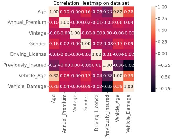
- Data normalization and splitting with test_size=0.3
# Find index of feature columns with correlation greater than 0.80
to_drop = [column for column in upper.columns if any(upper[column].abs() > 0.80)]
to_drop
['Vehicle_Age', 'Vehicle_Damage']

# Drop features
X_all_c = X_all_v.drop(X_all_v[to_drop], axis=1)

# Normalization
scaling = MinMaxScaler()
# Normalization of numerical features
num_sc = pd.DataFrame(scaling.fit_transform(X_all_c[['Age','Annual_Premium','Vintage']]), columns= ['Age','Annual_Premium','Vintage'])
# Grasp all
X_all_sc = pd.concat([num_sc, X_all_c[['Gender','Driving_License','Previously_Insured']]], axis=1)

# Split data set
# Break off train and test set from data
X_train, X_test, y_train, y_test = train_test_split(X_all_sc, y, train_size=0.7, test_size=0.3,stratify=y,random_state=0)
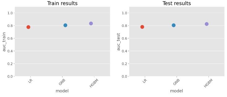
- Comparing several ML models in terms of the training time and AUC score
# LR model
start = time.time()
skf = StratifiedKFold(n_splits=5,random_state=0, shuffle=True)
LR = LogisticRegression(random_state=0)

param_grid = {}
LR_model = GridSearchCV(LR,param_grid,cv=skf)
LR_classifier = LR_model.fit(X_train, y_train)
predictions_tr = LR_classifier.predict_proba(X_train)[:, 1]
predictions_t = LR_classifier.predict_proba(X_test)[:, 1]
LR_auc_train = roc_auc_score(y_train, predictions_tr)
LR_auc_test = roc_auc_score(y_test, predictions_t)
score= {'model':['LR'], 'auc_train':[LR_auc_train],'auc_test':[LR_auc_test]}
LR_score= pd.DataFrame(score)
stop = time.time()
print(f"Training time: {stop - start}s")

Training time: 1.8592848777770996s
LR_score
model	auc_train	auc_test
0	LR	0.778631	0.780518
# GNB model
start = time.time()
skf = StratifiedKFold(n_splits=5,random_state=0, shuffle=True)
GNB= GaussianNB()
param_grid = {}
GNB_model = GridSearchCV(GNB,param_grid,cv=skf)
GNB_classifier = GNB_model.fit(X_train, y_train)
predictions_tr = GNB_classifier.predict_proba(X_train)[:, 1]
predictions_t = GNB_classifier.predict_proba(X_test)[:, 1]
GNB_auc_train = roc_auc_score(y_train, predictions_tr)
GNB_auc_test = roc_auc_score(y_test, predictions_t)
score= {'model':['GNB'], 'auc_train':[GNB_auc_train],'auc_test':[GNB_auc_test]}
GNB_score= pd.DataFrame(score)
stop = time.time()
print(f"Training time: {stop - start}s")

Training time: 0.478222131729126s

GNB_score

model	auc_train	auc_test
0	GNB	0.804705	0.804968
# HGBM model
start = time.time()
skf = StratifiedKFold(n_splits=5,random_state=0, shuffle=True)
HGBM= HistGradientBoostingClassifier(random_state=0)
param_grid = {}
HGBM_model = GridSearchCV(HGBM,param_grid,cv=skf)
HGBM_classifier = HGBM_model.fit(X_train, y_train)
predictions_tr = HGBM_classifier.predict_proba(X_train)[:, 1]
predictions_t = HGBM_classifier.predict_proba(X_test)[:, 1]
HGBM_auc_train = roc_auc_score(y_train, predictions_tr)
HGBM_auc_test = roc_auc_score(y_test, predictions_t)
score= {'model':['HGBM'], 'auc_train':[HGBM_auc_train],'auc_test':[HGBM_auc_test]}
HGBM_score= pd.DataFrame(score)
stop = time.time()
print(f"Training time: {stop - start}s")

Training time: 5.101318597793579s

HGBM_score

model	   auc_train	auc_test
0	HGBM	0.833247	0.826952
- Comparing AUC scores for both train and test data
score_cal = LR_score.append(GNB_score)
score_cal = score_cal.append(HGBM_score)
score_cal

model	   auc_train	auc_test
0	LR	    0.778631	0.780518
0	GNB	    0.804724	0.804944
0	HGBM	0.833247	0.826952
# Plot results for a graphical comparison
print("Spot Check Models")
plt.rcParams['figure.figsize']=(15,5)
plt.figure()
plt.subplot(1,2,1)
sns.stripplot(x="model", y="auc_train",data=score_cal,size=15)
plt.xticks(rotation=45)
plt.title('Train results')
axes = plt.gca()
axes.set_ylim([0,1.1])
plt.subplot(1,2,2)
sns.stripplot(x="model", y="auc_test",data=score_cal,size=15)
plt.xticks(rotation=45)
plt.title('Test results')
axes = plt.gca()
axes.set_ylim([0,1.1])
plt.show()

Spot Check Models
- Implementing the HGBM model tuning and AUC, ROC, f1 validation
#Tuning
start = time.time()
# cross validation
skf = StratifiedKFold(n_splits=5, random_state=0, shuffle=True)
# define models and hyperparameters
HGBM = HistGradientBoostingClassifier(random_state=0)
# define grid search
hyp_space = {"max_depth": [10,21],
             "learning_rate": [0.02,0.5],
             "max_bins": [80, 195]}
# Tuning and fit the model
HGBM_model_ = GridSearchCV(HGBM, hyp_space, n_jobs=-1, cv=skf, scoring='roc_auc', error_score=0).fit(X_train, y_train)
stop = time.time()
print(f"Training time: {stop-start}s")

Training time: 25.615475177764893s
def display(results):
    print(f'Best parameters are: {results.best_params_}')
    print("\n")
    mean_score = results.cv_results_['mean_test_score']
    std_score = results.cv_results_['std_test_score']
    params = results.cv_results_['params']
    for mean,std,params in zip(mean_score,std_score,params):
        print(f'{round(mean,3)} + or -{round(std,3)} for the {params}')

display(HGBM_model_)

Best parameters are: {'learning_rate': 0.02, 'max_bins': 80, 'max_depth': 10}


0.827 + or -0.002 for the {'learning_rate': 0.02, 'max_bins': 80, 'max_depth': 10}
0.827 + or -0.002 for the {'learning_rate': 0.02, 'max_bins': 80, 'max_depth': 21}
0.827 + or -0.002 for the {'learning_rate': 0.02, 'max_bins': 195, 'max_depth': 10}
0.827 + or -0.002 for the {'learning_rate': 0.02, 'max_bins': 195, 'max_depth': 21}
0.825 + or -0.002 for the {'learning_rate': 0.5, 'max_bins': 80, 'max_depth': 10}
0.825 + or -0.002 for the {'learning_rate': 0.5, 'max_bins': 80, 'max_depth': 21}
0.824 + or -0.002 for the {'learning_rate': 0.5, 'max_bins': 195, 'max_depth': 10}
0.825 + or -0.002 for the {'learning_rate': 0.5, 'max_bins': 195, 'max_depth': 21}
# HGBM Model Training
HGBM_ = HistGradientBoostingClassifier(random_state=0,learning_rate=0.02, max_bins=80, max_depth= 10)

# fit the model
HGBM_tclassifier = HGBM_.fit(X_train, y_train)

start = time.time()
# prediction
predictions_tr = HGBM_tclassifier.predict_proba(X_train)[:, 1]
predictions_tr_ = pd.DataFrame(predictions_tr, columns=['y_train_pred'])
predictions_te = HGBM_tclassifier.predict_proba(X_test)[:, 1]
predictions_te_ = pd.DataFrame(predictions_te, columns=['y_test_pred'])
stop = time.time()
print(f"Training time: {stop-start}s")

Training time: 0.581667423248291s

auc_train = roc_auc_score(y_train, HGBM_tclassifier.predict_proba(X_train)[:, 1])
auc_test = roc_auc_score(y_test, HGBM_tclassifier.predict_proba(X_test)[:, 1])

# metrics table
d1 = {'evaluation': ['AUC'],
     'model': ['HGBM'],
    'train': [auc_train],
    'test': [auc_test]
        }
df1 = pd.DataFrame(data=d1, columns=['model','evaluation','train','test'])
print('HGBM evaluation on cross-sell prediction')
df1

HGBM evaluation on cross-sell prediction

model	   evaluation	train	test
0	HGBM	AUC	      0.829556	0.827226

# Use f1_score to maximize
metric = f1_score

# Generate a range of classification thresholds to evaluate
thresholds = np.arange(0.0, 1.01, 0.01)

# Compute the metric for each threshold
metric_values = [metric(y_test, np.where(predictions_te >= threshold, 1, 0)) for threshold in thresholds]

# Find the best threshold that maximizes the metric
best_threshold = thresholds[np.argmax(metric_values)]

print("Best threshold:", best_threshold)

Best threshold: 0.21
- Plotting the HGBM ROC Curve
# compute the tpr and fpr from the prediction
fpr, tpr, thresholds = roc_curve(y_test, predictions_te)

# Plot the ROC curve
plt.rcParams['figure.figsize']=(10,5)
plt.plot(fpr, tpr, label='ROC Curve (AUC = %0.2f)' % auc(fpr, tpr))
plt.plot([0, 1], [0, 1], 'k--')
plt.xlim([0.0, 1.0])
plt.ylim([0.0, 1.05])
plt.xlabel('False Positive Rate')
plt.ylabel('True Positive Rate')
plt.title('Receiver Operating Characteristic (ROC) Curve')
plt.legend(loc="lower right")

# Adjust the threshold and compute the true positive rate (TPR) and false positive rate (FPR)
threshold = 0.21
y_pred = np.where(predictions_te >= threshold, 1, 0)
fpr_new, tpr_new, _ = roc_curve(y_test, y_pred)

# Plot the new point on the ROC curve
plt.scatter(fpr_new, tpr_new, c='r', label='New Threshold = %0.2f' % threshold)
plt.legend(loc="lower right")
print('ROC on test')
plt.show()

ROC on test

- Comparing true vs predicted test values
# create a barplot for a comparison between test values and predicted values
y_test_= np.array(y_test)
y_test_ = y_test_.flatten()
y_pred = y_pred.flatten()
df_2 = pd.DataFrame({'Actual': y_test_, 'Predicted': y_pred})
sns.countplot(x='value', hue='variable', data=pd.melt(df_2))
plt.title('True vs Predicted Labels')
plt.show()

- Plotting the SHAP HGBM model interpreter
HGBM_explainer = shap.TreeExplainer(HistGradientBoostingClassifier(random_state=0,learning_rate=0.02, max_bins=80, max_depth= 10).fit(X_train, y_train))
shap_values = HGBM_explainer.shap_values(X_test)
# Global SHAP on test
print("HGBM SHAP BARPLOT on test Values")
shap.summary_plot(shap_values, features=X_test, feature_names=X_test.columns,plot_type='bar')

XGB Model Validation
- Let’s train and validate the XGBoost model
# Import key libraries

import pandas as pd, numpy as np
import os
import math
from math import ceil, floor, log
import random

from sklearn.model_selection import KFold
import matplotlib.pyplot as plt
from sklearn.metrics import confusion_matrix, accuracy_score
from sklearn.metrics import f1_score, roc_auc_score, confusion_matrix, precision_recall_curve, auc, roc_curve, recall_score, classification_report
from sklearn.model_selection import train_test_split
import sklearn
from sklearn import metrics
from sklearn import preprocessing
from sklearn.linear_model import LogisticRegression
from sklearn.ensemble import RandomForestClassifier

import seaborn as sns

from yellowbrick.classifier import ClassificationReport
import scikitplot as skplt

from xgboost import XGBClassifier
import xgboost as xgb
from lightgbm import LGBMClassifier
import catboost
print(catboost.__version__)
from catboost import *
from catboost import datasets
from catboost import CatBoostClassifier

import scikitplot as skplt
1.1.1
- Data preparation
SEED = 1970
random.seed(SEED)
df_train = pd.read_csv("train.csv")
df_test = pd.read_csv("test.csv")

col_list = df_train.columns.to_list()[1:]
df_train_corr = df_train.copy().set_index('id')
df_train_ones = df_train_corr.loc[df_train_corr.Response == 1].copy()

categorical_features = ['Gender', 'Driving_License', 'Region_Code', 'Previously_Insured', 'Vehicle_Age', 'Vehicle_Damage','Policy_Sales_Channel']
text_features = ['Gender', 'Vehicle_Age', 'Vehicle_Damage']

# code text categorical features
le = preprocessing.LabelEncoder()
for f in text_features :
    df_train_corr[f] = le.fit_transform(df_train_corr[f])
# change digital categorical datatype so CatBoost can deal with them
df_train_corr.Region_Code = df_train_corr.Region_Code.astype('int32')
df_train_corr.Policy_Sales_Channel = df_train_corr.Policy_Sales_Channel.astype('int32')

def plot_ROC(fpr, tpr, m_name):
    roc_auc = sklearn.metrics.auc(fpr, tpr)
    plt.figure(figsize=(6, 6))
    lw = 2
    plt.plot(fpr, tpr, color='darkorange',
             lw=lw, label='ROC curve (area = %0.2f)' % roc_auc, alpha=0.5)

    plt.plot([0, 1], [0, 1], color='navy', lw=lw, linestyle='--', alpha=0.5)

    plt.xlim([0.0, 1.0])
    plt.ylim([0.0, 1.05])
    plt.xticks(fontsize=16)
    plt.yticks(fontsize=16)
    plt.grid(True)
    plt.xlabel('False Positive Rate', fontsize=16)
    plt.ylabel('True Positive Rate', fontsize=16)
    plt.title('Receiver operating characteristic for %s'%m_name, fontsize=20)
    plt.legend(loc="lower right", fontsize=16)
    plt.show()

def upsample(df, u_feature, n_upsampling):
    ones = df.copy()
    for n in range(n_upsampling):
        if u_feature == 'Annual_Premium':
            df[u_feature] = ones[u_feature].apply(lambda x: x + random.randint(-1,1)* x *0.05) # change Annual_premiun in the range of 5%
        else:
            df[u_feature] = ones[u_feature].apply(lambda x: x + random.randint(-5,5)) # change Age in the range of 5 years

        if n == 0:
            df_new = df.copy()
        else:
            df_new = pd.concat([df_new, df])
    return df_new

try:
    df_train_corr.drop(columns = ['bin_age'], inplace = True)
except:
    print('already deleted')

df_train_mod = df_train_corr.copy()
df_train_mod['old_damaged'] = df_train_mod.apply(lambda x: pow(2,x.Vehicle_Age)+pow(2,x.Vehicle_Damage), axis =1)

# we shall preserve validation set without augmentation/over-sampling
df_temp, X_valid, _, y_valid = train_test_split(df_train_mod, df_train_mod['Response'], train_size=0.8, random_state = SEED)
X_valid = X_valid.drop(columns = ['Response'])

# upsampling Positive Response class only
df_train_up_a = upsample(df_temp.loc[df_temp['Response'] == 1], 'Age', 1)
df_train_up_v = upsample(df_temp.loc[df_temp['Response'] == 1], 'Vintage', 1)

df_ext = pd.concat([df_train_mod,df_train_up_a])
df_ext = pd.concat([df_ext,df_train_up_v])
X_train = df_ext.drop(columns = ['Response'])
y_train = df_ext.Response
print('Train set target class count with over-sampling:')
print(y_train.value_counts())
print('Validation set target class count: ')
print(y_valid.value_counts())
X_train.head()

Train set target class count with over-sampling:
0    334399
1    121390
Name: Response, dtype: int64
Validation set target class count:
0    66852
1     9370
Name: Response, dtype: int64
- Fitting the XGBoost Classifier
XGB_model_l = XGBClassifier(random_state = SEED, max_depth = 8,
                            n_estimators = 30000,
                            reg_lambda = 1.2, reg_alpha = 1.2,
                            min_child_weight = 1,
                            objective = 'binary:logistic',
                            learning_rate = 0.15, gamma = 0.3, colsample_bytree = 0.5, eval_metric = 'auc')

XGB_model_l.fit(X_train, y_train,
                eval_set = [(X_valid, y_valid)],
                early_stopping_rounds=50,verbose = 1000)
[0]	validation_0-auc:0.75188
[1000]	validation_0-auc:0.90154
[2000]	validation_0-auc:0.92239
[3000]	validation_0-auc:0.93506
[4000]	validation_0-auc:0.94647
[5000]	validation_0-auc:0.95441
[6000]	validation_0-auc:0.96068
[7000]	validation_0-auc:0.96629
[8000]	validation_0-auc:0.97081
[9000]	validation_0-auc:0.97479
[10000]	validation_0-auc:0.97813
[11000]	validation_0-auc:0.98071
[12000]	validation_0-auc:0.98277
[13000]	validation_0-auc:0.98462
[14000]	validation_0-auc:0.98639
[15000]	validation_0-auc:0.98796
[16000]	validation_0-auc:0.98918
[17000]	validation_0-auc:0.99025
[18000]	validation_0-auc:0.99115
[19000]	validation_0-auc:0.99189
[20000]	validation_0-auc:0.99260
[21000]	validation_0-auc:0.99323
[22000]	validation_0-auc:0.99378
[23000]	validation_0-auc:0.99429
[24000]	validation_0-auc:0.99476
[25000]	validation_0-auc:0.99515
[26000]	validation_0-auc:0.99550
[27000]	validation_0-auc:0.99579
[28000]	validation_0-auc:0.99600
[29000]	validation_0-auc:0.99622
[29999]	validation_0-auc:0.99643

XGBClassifier(base_score=0.5, booster='gbtree', callbacks=None,
              colsample_bylevel=1, colsample_bynode=1, colsample_bytree=0.5,
              early_stopping_rounds=None, enable_categorical=False,
              eval_metric='auc', feature_types=None, gamma=0.3, gpu_id=-1,
              grow_policy='depthwise', importance_type=None,
              interaction_constraints='', learning_rate=0.15, max_bin=256,
              max_cat_threshold=64, max_cat_to_onehot=4, max_delta_step=0,
              max_depth=8, max_leaves=0, min_child_weight=1, missing=nan,
              monotone_constraints='()', n_estimators=30000, n_jobs=0,
              num_parallel_tree=1, predictor='auto', random_state=1970, ...)
XGB_preds_l = XGB_model_l.predict_proba(X_valid)
XGB_score_l = roc_auc_score(y_valid, XGB_preds_l[:,1])
XGB_class_l = XGB_model_l.predict(X_valid)
- XGBoost model validation
(fpr, tpr, thresholds) = roc_curve(y_valid, XGB_preds_l[:,1])
plt.rcParams.update({'font.size': 22})
plot_ROC(fpr, tpr,'XGBoost')

print('ROC AUC score for XGBoost model with over-sampling + 2 new features: %.4f'%XGB_score_l)
print('F1 score: %0.4f'%f1_score(y_valid, XGB_class_l))
skplt.metrics.plot_confusion_matrix(y_valid, XGB_class_l,
        figsize=(8,8))

xgb.plot_importance(XGB_model_l)
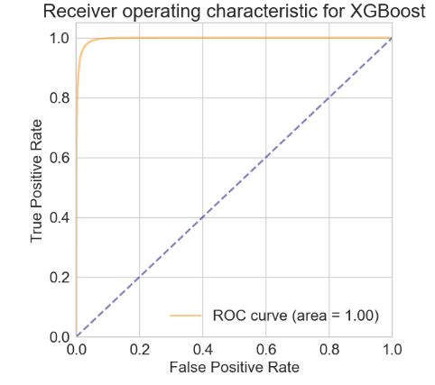
- ROC AUC score for XGBoost model with over-sampling + 2 new features: 0.9964 F1 score: 0.9176

- Plotting the XGBoost normalized confusion matrix
from sklearn.metrics import confusion_matrix
import seaborn as sns

target_names=['0','1']
plt.rcParams.update({'font.size': 22})
cm = confusion_matrix(y_valid, XGB_class_l)
# Normalise
cmn = cm.astype('float') / cm.sum(axis=1)[:, np.newaxis]
fig, ax = plt.subplots(figsize=(10,10))
sns.heatmap(cmn, annot=True, fmt='.6f', xticklabels=target_names, yticklabels=target_names)
plt.ylabel('Actual',fontsize=18)
plt.xlabel('Predicted',fontsize=18)
plt.title('XGB Confusion Matrix',fontsize=18)
plt.show(block=False)

IQR Filtering & RF Modeling
- Following the recent study, we will investigate the impact of outlier removal via IQR filtering
import numpy as np
import pandas as pd
import matplotlib.pyplot as plt
import seaborn as sns
import warnings
warnings.filterwarnings('ignore')
df = pd.read_csv('train.csv')
onehots = pd.get_dummies(df['Vehicle_Age'], prefix='Vehicle_Age')
df = df.join(onehots)
onehots2 = pd.get_dummies(df['Gender'], prefix='Gender')
df = df.join(onehots2)
onehots3 = pd.get_dummies(df['Vehicle_Damage'], prefix='Vehicle_Damage')
df = df.join(onehots3)
df = df.drop(['id', 'Gender', 'Vehicle_Damage', 'Vehicle_Age'], axis=1)
print(f'Count of rows before filtering outlier: {len(df)}')

filtered_entries = np.array([True] * len(df))
for col in ['Annual_Premium']:
    Q1 = df[col].quantile(0.25)
    Q3 = df[col].quantile(0.75)
    IQR = Q3 - Q1
    low_limit = Q1 - (IQR * 1.5)
    high_limit = Q3 + (IQR * 1.5)

    filtered_entries = ((df[col] >= low_limit) & (df[col] <= high_limit)) & filtered_entries

df = df[filtered_entries]

print(f'Count of rows after filtering outlier: {len(df)}')
Count of rows before filtering outlier: 369067
Count of rows after filtering outlier: 369039

df = df.drop(['Annual_Premium'], axis=1)
print(df['Response'].value_counts())
0    324365
1     44914
Name: Response, dtype: int64

X = df[[col for col in df.columns if (str(df[col].dtype) != 'object') and col not in ['Response']]]
y = df['Response'].values
print(X.shape)
print(y.shape)
(369279, 14)
(369279,)

from imblearn import over_sampling
X_over, y_over = over_sampling.RandomOverSampler().fit_resample(X, y)
df_y_over = pd.Series(y_over).value_counts()
df_y_over
1    324365
0    324365
dtype: int64

df.to_csv('train_pre_processed.csv')
- Applying the RF Classifier to the filtered dataset
from sklearn.ensemble import RandomForestClassifier
# Split Feature Vector and Label
X = df.drop(['Response'], axis = 1) # menggunakan semua feature kecuali target
y = df['Response'] # target / label

#Splitting the data into Train and Test
from sklearn.model_selection import train_test_split
X_train, X_test,y_train,y_test = train_test_split(X,
                                                y,
                                                test_size = 0.3,
                                                random_state = 789)
rf = RandomForestClassifier(n_estimators= 400, max_depth=110, random_state=0)
rf.fit(X_train, y_train)
RandomForestClassifier(max_depth=110, n_estimators=400, random_state=0)

y_predicted = rf.predict(X_test)
- Final RF classification report
# OUTLIERS throwed away
# Data oversampled on Response == 1

from sklearn.metrics import classification_report, confusion_matrix, accuracy_score, precision_score
print('\nconfustion matrix') # generate the confusion matrix
print(confusion_matrix(y_test, y_predicted))

print('\naccuracy')
print(accuracy_score(y_test, y_predicted))
print('\nprecision')
print(precision_score(y_test, y_predicted))


print('\nclassification report')
print(classification_report(y_test, y_predicted))

confustion matrix
[[85995 11312]
 [  300 97012]]

accuracy
0.9403347052446062

precision
0.8955725416343562

classification report
              precision    recall  f1-score   support

           0       1.00      0.88      0.94     97307
           1       0.90      1.00      0.94     97312

    accuracy                           0.94    194619
   macro avg       0.95      0.94      0.94    194619
weighted avg       0.95      0.94      0.94    194619

print("train Accuracy : ",rf.score(X_train,y_train))
print("test Accuracy : ",rf.score(X_test,y_test))
train Accuracy :  0.9999229263329891
test Accuracy :  0.9403347052446062
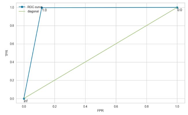
from sklearn.metrics import roc_curve, auc
fpr, tpr, thresholds = roc_curve(y_test, y_predicted, pos_label=1) # pos_label: label yang kita anggap positive
print('Area Under ROC Curve (AUC):', auc(fpr, tpr))

Area Under ROC Curve (AUC): 0.9403332515355389
plt.subplots(figsize=(10, 6))
plt.plot(fpr, tpr, 'o-', label="ROC curve")
plt.plot(np.linspace(0,1,10), np.linspace(0,1,10), label="diagonal")
for x, y, txt in zip(fpr, tpr, thresholds):
    plt.annotate(np.round(txt,2), (x, y-0.04))
plt.legend(loc="upper left")
plt.xlabel("FPR")
plt.ylabel("TPR")
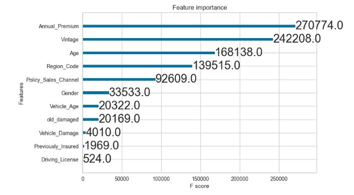
# RF feature importance score

feat_importances = pd.Series(rf.feature_importances_, index=X.columns)
ax = feat_importances.nlargest(10).plot(kind='barh')
ax.invert_yaxis()
plt.xlabel('score')
plt.ylabel('feature')
plt.title('feature importance score')

- Final RF normalized confusion matrix
from sklearn.metrics import confusion_matrix
import seaborn as sns

target_names=['0','1']

cm = confusion_matrix(y_test, y_predicted)
# Normalise
cmn = cm.astype('float') / cm.sum(axis=1)[:, np.newaxis]
fig, ax = plt.subplots(figsize=(10,10))
sns.heatmap(cmn, annot=True, fmt='.6f', xticklabels=target_names, yticklabels=target_names)
plt.ylabel('Actual')
plt.xlabel('Predicted')
plt.show(block=False)

Conclusions
- In this project, we have applied supervised binary classification and AI-powered predictive analytics to cross-selling insurance initiatives.
- We have proposed an integrated ML approach for identifying cross-sell opportunities within insurance customer data using ML model tuning, cross-validation & interpretation.
- This approach has been extensively tested and evaluated on real insurance data that had been provided by an insurance company.
- Results show the ability of ML tuning pipelines, and ensemble models (HGBM, XGBoost, and Random Forest) to identify cross-sell customers.
- The study will be integrated into a recommendation system that can be used to assign cross-sell probability scores to current or new insurance customers, to support advisors for improved cross product selling.
References
- Health Insurance Cross Sell Prediction
- Model Building Example – Section 11
- Scikit-Plot: Visualize ML Model Performance Evaluation Metrics
- Insurance_Cross_Sell_Prediction
- Insurance Prediction, RandomForest, AUC-99
- Customer Behavior Prediction(AUC: 85%)
- Where is the problem? AUC score reached 99.7%
- Cross Sell w/ 0.946 AUC & 90% potential Conversion
Explore More
- Telco Customer Churn/Retention Rate ML/AI Strategies that Work!
- ML/AI Credit Risk Analytics
- Unsupervised ML Clustering, Customer Segmentation, Cohort, Market Basket, Bank Churn, CRM, ABC & RFM Analysis – A Comprehensive Guide in Python
- Advanced Integrated Data Visualization (AIDV) in Python – 2. Dabl Auto EDA & ML


One-Time
Monthly
Yearly
Make a one-time donation
Make a monthly donation
Make a yearly donation
Choose an amount
€5.00
€15.00
€100.00
€5.00
€15.00
€100.00
€5.00
€15.00
€100.00
Or enter a custom amount
€
Your contribution is appreciated.
Your contribution is appreciated.
Your contribution is appreciated.
DonateDonate monthlyDonate yearly
Leave a comment