
Featured Photo of Karolina Grabowska on Pexels.
- Cardiovascular disease (CVD) is the principal cause of mortality and morbidity globally. With the pressures for improved care and translation of the latest medical advances and knowledge to an actionable plan, clinical decision-making for cardiologists is challenging.
- This scope of this project is within the AI-driven Cardiovascular Medicine. Specifically, it will focus on early diagnosis of heart disease using Artificial Neural Networks (ANN).
- The ANN method aims to improve the detection of heart issues, which could lead to better outcomes since early diagnosis is critical.
- This project will utilize a dataset of 303 patients and distributed by the UCI Machine Learning Repository.
Data Preparation
Let’s set the working directory HEART23
import os
os.chdir(‘HEART23’)
os. getcwd()
and import the libraries
import pandas as pd
import numpy as np
import matplotlib.pyplot as plt
import seaborn as sns
sns.set()
from scipy.stats import skew
from sklearn.preprocessing import StandardScaler
from sklearn.model_selection import train_test_split
from sklearn.metrics import accuracy_score, roc_curve, roc_auc_score, precision_score, recall_score
import scikitplot as skplt
import tensorflow as tf
Let’s read the input data
data = pd.read_csv(‘heartcvd.csv’)
data.head()
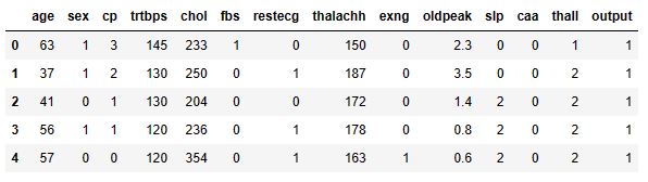
where output of 0 means that a person has a low chance of CVD while 1 suggests that the person has a high chance of CVD.
Let’s check the data structure:
print(f’Number of rows:’, data.shape[0])
print(f’Number of columns:’, data.shape[1])
Number of rows: 303
Number of columns: 14
We have 5 numerical features and 8 categorical features in our dataset
data.nunique()
age          41
sex           2
cp            4
trtbps       49
chol        152
fbs           2
restecg       3
thalachh     91
exng          2
oldpeak      40
slp           3
caa           5
thall         4
output        2
dtype: int64
data.info()
<class 'pandas.core.frame.DataFrame'>
RangeIndex: 303 entries, 0 to 302
Data columns (total 14 columns):
 #   Column    Non-Null Count  Dtype
---  ------    --------------  -----
 0   age       303 non-null    int64
 1   sex       303 non-null    int64
 2   cp        303 non-null    int64
 3   trtbps    303 non-null    int64
 4   chol      303 non-null    int64
 5   fbs       303 non-null    int64
 6   restecg   303 non-null    int64
 7   thalachh  303 non-null    int64
 8   exng      303 non-null    int64
 9   oldpeak   303 non-null    float64
 10  slp       303 non-null    int64
 11  caa       303 non-null    int64
 12  thall     303 non-null    int64
 13  output    303 non-null    int64
dtypes: float64(1), int64(13)
memory usage: 33.3 KB
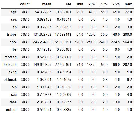
data.describe().T
All of our categorical columns have an integer datatype. I will convert them into an object datatype
cat_columns = [‘sex’, ‘cp’, ‘fbs’, ‘restecg’, ‘exng’, ‘slp’, ‘caa’, ‘thall’, ‘output’]
num_columns = [‘age’, ‘trtbps’, ‘oldpeak’, ‘chol’, ‘thalachh’]
data[cat_columns] = data[cat_columns].astype(str)
Let’s see if we don’t have any missing values in our dataset
data.isnull().sum()
age         0
sex         0
cp          0
trtbps      0
chol        0
fbs         0
restecg     0
thalachh    0
exng        0
oldpeak     0
slp         0
caa         0
thall       0
output      0
dtype: int64
Exploratory Data Analysis (EDA)
Let's compare distributions of various features based on target variable
sns.set_context(‘notebook’, font_scale= 1.2)
fig, ax = plt.subplots(2, 2, figsize = (20, 13))
plt.suptitle(‘Distribution of various features based on target variable’, fontsize = 20)
ax1 = sns.histplot(x =’age’, data= data, hue= ‘output’, kde= True, ax= ax[0, 0], palette=’winter’)
ax1.set(xlabel = ‘Age’, title= ‘Distribution of age based on target variable’)
ax2 = sns.histplot(x =’trtbps’, data= data, hue= ‘output’, kde= True, ax= ax[0, 1], palette=’plasma’)
ax2.set(xlabel = ‘Resting blood pressure (in mm Hg)’, title= ‘Distribution of BP based on target variable’)
ax3 = sns.histplot(x =’chol’, data= data, hue= ‘output’, kde= True, ax= ax[1, 0], palette=’winter’)
ax3.set(xlabel = ‘Cholesterol in mg/dl’, title= ‘Distribution of Cholesterol based on target variable’)
ax4 = sns.histplot(x =’thalachh’, data= data, hue= ‘output’, kde= True, ax= ax[1, 1], palette=’plasma’)
ax4.set(xlabel = ‘Max Heart Rate Achieved’, title= ‘Distribution of maximum heart rate achieved based on target variable’)
plt.show()

We can see a pattern in the distribution of maximum heart rate achieved. Those who have reached a higher maximum heart rate are more likely to have CVD.
Let’s compare boxplots of various features based on target variable
sns.set_context(‘notebook’, font_scale= 1.2)
fig, ax = plt.subplots(2, 2, figsize = (20, 10))
plt.suptitle(‘Boxplot of various features based on target variable’, fontsize = 20)
ax1 = sns.boxplot(x =’age’, data= data, ax= ax[0, 0], color = ‘#40bf80’)
ax1.set(xlabel = ‘Age’)
ax2 = sns.boxplot(x =’trtbps’, data= data, ax= ax[0, 1], color=’#40bf80′)
ax2.set(xlabel = ‘Resting blood pressure (in mm Hg)’)
ax3 = sns.boxplot(x =’chol’, data= data, hue= ‘output’, ax= ax[1, 0], color= ‘#40bf80’)
ax3.set(xlabel = ‘Cholesterol in mg/dl’)
ax4 = sns.boxplot(x =’thalachh’, data= data, ax= ax[1, 1], color = ‘#40bf80’)
ax4.set(xlabel = ‘Max Heart Rate Achieved’)
plt.savefig(‘cvd1boxplotstarget.png’)

There are some outliers in the Blood Pressure and Cholesterol columns.
Let’s look at the feature correlations using the sns heatmap
plt.figure(figsize= (16, 8))
sns.heatmap(data.corr(), annot = True, cmap= ‘YlGnBu’, fmt= ‘.2f’);

I don’t think there is any correlation between our numerical features.
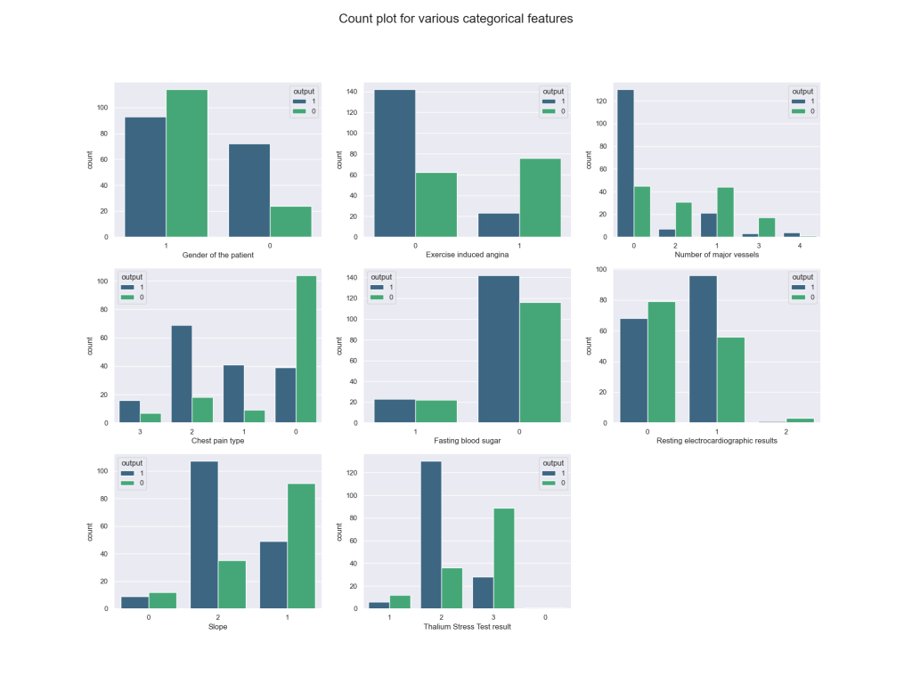
Let’s compare count plots for various categorical features
sns.set_context(‘notebook’, font_scale= 1)
fig, ax = plt.subplots(3, 3, figsize = (20, 15))
ax[2, 2].axis(‘off’)
plt.suptitle(‘Count plot for various categorical features’, fontsize = 20)
ax1 = sns.countplot(x =’sex’, data= data, ax= ax[0, 0], hue = ‘output’ ,palette= ‘viridis’)
ax1.set(xlabel = ‘Gender of the patient’)
ax2 = sns.countplot(x =’exng’, data= data, hue= ‘output’, ax= ax[0, 1], palette= ‘viridis’)
ax2.set(xlabel = ‘Exercise induced angina’)
ax3 = sns.countplot(x =’caa’, data= data, ax= ax[0, 2], hue = ‘output’, palette= ‘viridis’)
ax3.set(xlabel = ‘Number of major vessels’)
ax4 = sns.countplot(x =’cp’, data= data, hue = ‘output’, ax= ax[1, 0], palette= ‘viridis’)
ax4.set(xlabel = ‘Chest pain type’)
ax5 = sns.countplot(x =’fbs’, data= data, hue = ‘output’, ax= ax[1, 1], palette= ‘viridis’)
ax5.set(xlabel = ‘Fasting blood sugar’)
ax6 = sns.countplot(x =’restecg’, data= data, ax= ax[1, 2], hue = ‘output’, palette= ‘viridis’)
ax6.set(xlabel = ‘Resting electrocardiographic results’)
ax7 = sns.countplot(x =’slp’, data= data, ax= ax[2, 0], hue = ‘output’, palette= ‘viridis’)
ax7.set(xlabel = ‘Slope’)
ax8 = sns.countplot(x =’thall’, data= data, ax= ax[2, 1], hue = ‘output’, palette= ‘viridis’)
ax8.set(xlabel = ‘Thalium Stress Test result’)
plt.show()
data[‘output’].value_counts()
1    165
0    138
Name: output, dtype: int64
plt.figure(figsize= (6, 8))
data_pie = [165 , 138]
labels = [“High Chances”, “Low Chances”]
explode = [0.1, 0]
plt.pie(data_pie ,labels= labels , explode = explode , autopct=”%1.2f%%”, shadow= True, colors= [‘#256D85’, ‘#3BACB6’])
plt.show()

This is a well balanced dataset.
Checking for skewness:
def skewness(data):
skew_df = pd.DataFrame(data.select_dtypes(np.number).columns, columns=[‘Feature’])
skew_df[‘Skew’] = skew_df[‘Feature’].apply(lambda feature: skew(data[feature]))
skew_df[‘Absolute Skew’] = skew_df[‘Skew’].apply(abs)
return skew_df
skewness(data=data[num_columns])

Since oldpeak and chol columns are skewed, we will apply the log transformation
data[‘oldpeak’] = np.log1p(data[‘oldpeak’])
data[‘chol’] = np.log1p(data[‘chol’])
data = pd.get_dummies(data, drop_first=True)
data.head()

Train/Test Data
Let’s prepare our data for DL using StandardScaler and train_test_split with test_size= 0.20
X = data.drop(‘output_1’, axis= 1)
y = data.output_1
scaler = StandardScaler()
X = scaler.fit_transform(X)
X_train, X_test, y_train, y_test = train_test_split(X, y, test_size= 0.20,random_state= 42)
print(X_train.shape)
(242, 22)
Training Sequential ANN
model = tf.keras.Sequential([
tf.keras.Input(22),
tf.keras.layers.Dense(100, activation = ‘relu’),
tf.keras.layers.Dropout(0.2),
tf.keras.layers.Dense(1, activation = ‘sigmoid’)
])
model.compile(
loss = tf.keras.losses.BinaryCrossentropy(),
optimizer = tf.keras.optimizers.Adam(),
metrics=[tf.keras.metrics.AUC(name=’auc’)]
)
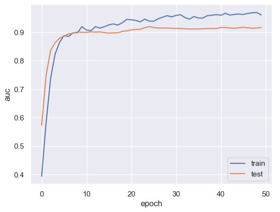
history = model.fit(X_train, y_train, epochs = 50, validation_split = 0.20)
Epoch 1/50
7/7 [==============================] - 1s 33ms/step - loss: 0.7810 - auc: 0.3940 - val_loss: 0.6786 - val_auc: 0.5731
Epoch 2/50
7/7 [==============================] - 0s 5ms/step - loss: 0.6791 - auc: 0.5831 - val_loss: 0.6047 - val_auc: 0.7491
Epoch 3/50
7/7 [==============================] - 0s 5ms/step - loss: 0.6081 - auc: 0.7379 - val_loss: 0.5497 - val_auc: 0.8367
Epoch 4/50
7/7 [==============================] - 0s 5ms/step - loss: 0.5510 - auc: 0.8235 - val_loss: 0.5123 - val_auc: 0.8631
Epoch 5/50
7/7 [==============================] - 0s 5ms/step - loss: 0.5103 - auc: 0.8646 - val_loss: 0.4851 - val_auc: 0.8793
Epoch 6/50
7/7 [==============================] - 0s 5ms/step - loss: 0.4750 - auc: 0.8887 - val_loss: 0.4638 - val_auc: 0.8861
Epoch 7/50
7/7 [==============================] - 0s 5ms/step - loss: 0.4635 - auc: 0.8852 - val_loss: 0.4475 - val_auc: 0.8946
Epoch 8/50
7/7 [==============================] - 0s 5ms/step - loss: 0.4450 - auc: 0.8978 - val_loss: 0.4343 - val_auc: 0.8963
Epoch 9/50
7/7 [==============================] - 0s 5ms/step - loss: 0.4295 - auc: 0.8987 - val_loss: 0.4238 - val_auc: 0.9014
Epoch 10/50
7/7 [==============================] - 0s 5ms/step - loss: 0.4021 - auc: 0.9198 - val_loss: 0.4142 - val_auc: 0.8997
Epoch 11/50
7/7 [==============================] - 0s 5ms/step - loss: 0.4088 - auc: 0.9079 - val_loss: 0.4077 - val_auc: 0.8997
Epoch 12/50
7/7 [==============================] - 0s 5ms/step - loss: 0.4070 - auc: 0.9056 - val_loss: 0.4026 - val_auc: 0.9014
Epoch 13/50
7/7 [==============================] - 0s 5ms/step - loss: 0.3846 - auc: 0.9197 - val_loss: 0.3975 - val_auc: 0.9005
Epoch 14/50
7/7 [==============================] - 0s 4ms/step - loss: 0.3885 - auc: 0.9146 - val_loss: 0.3945 - val_auc: 0.9014
Epoch 15/50
7/7 [==============================] - 0s 5ms/step - loss: 0.3738 - auc: 0.9198 - val_loss: 0.3922 - val_auc: 0.8988
Epoch 16/50
7/7 [==============================] - 0s 5ms/step - loss: 0.3623 - auc: 0.9259 - val_loss: 0.3904 - val_auc: 0.8971
Epoch 17/50
7/7 [==============================] - 0s 5ms/step - loss: 0.3564 - auc: 0.9293 - val_loss: 0.3884 - val_auc: 0.8980
Epoch 18/50
7/7 [==============================] - 0s 5ms/step - loss: 0.3596 - auc: 0.9253 - val_loss: 0.3858 - val_auc: 0.8980
Epoch 19/50
7/7 [==============================] - 0s 4ms/step - loss: 0.3447 - auc: 0.9334 - val_loss: 0.3833 - val_auc: 0.9031
Epoch 20/50
7/7 [==============================] - 0s 4ms/step - loss: 0.3203 - auc: 0.9454 - val_loss: 0.3815 - val_auc: 0.9048
Epoch 21/50
7/7 [==============================] - 0s 5ms/step - loss: 0.3215 - auc: 0.9439 - val_loss: 0.3791 - val_auc: 0.9082
Epoch 22/50
7/7 [==============================] - 0s 5ms/step - loss: 0.3239 - auc: 0.9418 - val_loss: 0.3775 - val_auc: 0.9099
Epoch 23/50
7/7 [==============================] - 0s 5ms/step - loss: 0.3288 - auc: 0.9365 - val_loss: 0.3731 - val_auc: 0.9107
Epoch 24/50
7/7 [==============================] - 0s 5ms/step - loss: 0.3172 - auc: 0.9462 - val_loss: 0.3709 - val_auc: 0.9158
Epoch 25/50
7/7 [==============================] - 0s 5ms/step - loss: 0.3274 - auc: 0.9392 - val_loss: 0.3727 - val_auc: 0.9201
Epoch 26/50
7/7 [==============================] - 0s 5ms/step - loss: 0.3297 - auc: 0.9387 - val_loss: 0.3759 - val_auc: 0.9167
Epoch 27/50
7/7 [==============================] - 0s 5ms/step - loss: 0.3168 - auc: 0.9475 - val_loss: 0.3783 - val_auc: 0.9150
Epoch 28/50
7/7 [==============================] - 0s 5ms/step - loss: 0.3048 - auc: 0.9531 - val_loss: 0.3792 - val_auc: 0.9150
Epoch 29/50
7/7 [==============================] - 0s 5ms/step - loss: 0.2904 - auc: 0.9583 - val_loss: 0.3790 - val_auc: 0.9150
Epoch 30/50
7/7 [==============================] - 0s 5ms/step - loss: 0.2991 - auc: 0.9541 - val_loss: 0.3784 - val_auc: 0.9141
Epoch 31/50
7/7 [==============================] - 0s 5ms/step - loss: 0.2904 - auc: 0.9593 - val_loss: 0.3779 - val_auc: 0.9133
Epoch 32/50
7/7 [==============================] - 0s 5ms/step - loss: 0.2788 - auc: 0.9616 - val_loss: 0.3793 - val_auc: 0.9133
Epoch 33/50
7/7 [==============================] - 0s 5ms/step - loss: 0.2972 - auc: 0.9516 - val_loss: 0.3795 - val_auc: 0.9124
Epoch 34/50
7/7 [==============================] - 0s 5ms/step - loss: 0.3090 - auc: 0.9460 - val_loss: 0.3795 - val_auc: 0.9116
Epoch 35/50
7/7 [==============================] - 0s 5ms/step - loss: 0.2864 - auc: 0.9555 - val_loss: 0.3797 - val_auc: 0.9116
Epoch 36/50
7/7 [==============================] - 0s 5ms/step - loss: 0.2956 - auc: 0.9499 - val_loss: 0.3792 - val_auc: 0.9116
Epoch 37/50
7/7 [==============================] - 0s 5ms/step - loss: 0.2963 - auc: 0.9502 - val_loss: 0.3785 - val_auc: 0.9124
Epoch 38/50
7/7 [==============================] - 0s 5ms/step - loss: 0.2769 - auc: 0.9585 - val_loss: 0.3778 - val_auc: 0.9133
Epoch 39/50
7/7 [==============================] - 0s 4ms/step - loss: 0.2752 - auc: 0.9599 - val_loss: 0.3781 - val_auc: 0.9133
Epoch 40/50
7/7 [==============================] - 0s 5ms/step - loss: 0.2696 - auc: 0.9620 - val_loss: 0.3773 - val_auc: 0.9133
Epoch 41/50
7/7 [==============================] - 0s 4ms/step - loss: 0.2691 - auc: 0.9598 - val_loss: 0.3765 - val_auc: 0.9167
Epoch 42/50
7/7 [==============================] - 0s 5ms/step - loss: 0.2570 - auc: 0.9668 - val_loss: 0.3727 - val_auc: 0.9167
Epoch 43/50
7/7 [==============================] - 0s 4ms/step - loss: 0.2675 - auc: 0.9604 - val_loss: 0.3717 - val_auc: 0.9150
Epoch 44/50
7/7 [==============================] - 0s 4ms/step - loss: 0.2620 - auc: 0.9627 - val_loss: 0.3734 - val_auc: 0.9141
Epoch 45/50
7/7 [==============================] - 0s 4ms/step - loss: 0.2612 - auc: 0.9641 - val_loss: 0.3743 - val_auc: 0.9158
Epoch 46/50
7/7 [==============================] - 0s 5ms/step - loss: 0.2620 - auc: 0.9624 - val_loss: 0.3738 - val_auc: 0.9175
Epoch 47/50
7/7 [==============================] - 0s 5ms/step - loss: 0.2561 - auc: 0.9662 - val_loss: 0.3742 - val_auc: 0.9158
Epoch 48/50
7/7 [==============================] - 0s 5ms/step - loss: 0.2499 - auc: 0.9684 - val_loss: 0.3759 - val_auc: 0.9141
Epoch 49/50
7/7 [==============================] - 0s 4ms/step - loss: 0.2459 - auc: 0.9695 - val_loss: 0.3773 - val_auc: 0.9150
Epoch 50/50
7/7 [==============================] - 0s 5ms/step - loss: 0.2595 - auc: 0.9608 - val_loss: 0.3787 - val_auc: 0.9167
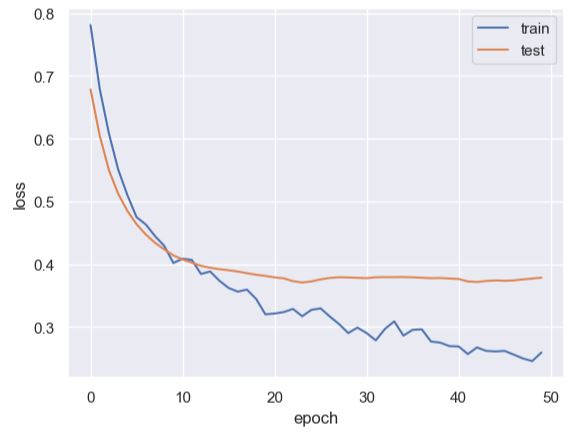
We can see the ANN output error values after 50 iterations: loss: 0.2595 – auc: 0.9608 – val_loss: 0.3787 – val_auc: 0.9167.
Let’s print our model
print(model.summary())
Model: "sequential"
_________________________________________________________________
 Layer (type)                Output Shape              Param #
=================================================================
 dense (Dense)               (None, 100)               2300

 dropout (Dropout)           (None, 100)               0

 dense_1 (Dense)             (None, 1)                 101

=================================================================
Total params: 2,401
Trainable params: 2,401
Non-trainable params: 0
_________________________________________________________________
None
Let’s check the train/test scores and accuracy values
scoret = model.evaluate(X_train, y_train, verbose=0)
print(‘Train score:’, scoret[0])
print(‘Train accuracy:’, scoret[1])
Train score: 0.26860886812210083
Train accuracy: 0.9574049711227417
score = model.evaluate(X_test, y_test, verbose=0)
print(‘Test score:’, score[0])
print(‘Test accuracy:’, score[1])
Test score: 0.3528120219707489
Test accuracy: 0.9224138259887695
ANN Model Validation
Let’s plot the content of history.keys()
print(history.history.keys())
dict_keys(['loss', 'auc', 'val_loss', 'val_auc'])
plt.plot(history.history[‘auc’])
plt.plot(history.history[‘val_auc’])
plt.legend([‘train’, ‘test’], loc=’lower right’)
plt.ylabel(‘auc’)
plt.xlabel(‘epoch’)
plt.plot(history.history[‘loss’])
plt.plot(history.history[‘val_loss’])
plt.legend([‘train’, ‘test’], loc=’upper right’)
plt.ylabel(‘loss’)
plt.xlabel(‘epoch’)
Let’s check our test predictions
pred = model.predict(X_test)
pred = tf.cast(tf.round(pred), dtype=tf.int32).numpy().reshape(61)
2/2 [==============================] - 0s 2ms/step
print(f’Accuracy of our model is {round(accuracy_score(y_test, pred) * 100, 2)}%’)
Accuracy of our model is 86.89%
print(f’Precision: {round(precision_score(y_test, pred), 2)}’)
Precision: 0.88
print(f’Recall: {round(recall_score(y_test, pred), 2)}’)
Recall: 0.88
Let’s plot the confusion matrix
skplt.metrics.plot_confusion_matrix(y_test,pred, figsize=(6,6), cmap= ‘YlGnBu’)

Let’s plot the ROC Curve
fpr, tpr, thresholds = roc_curve(y_test, pred)
plt.figure(figsize=(6,4))
plt.plot(fpr, tpr, linewidth=2, color= ‘teal’)
plt.plot([0,1], [0,1], ‘r–‘ )
plt.title(‘ROC Curve’)
plt.xlabel(‘False Positive Rate’)
plt.ylabel(‘True Positive Rate’)
plt.show()
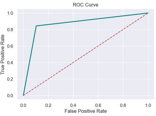
The ROC score is
roc_auc = roc_auc_score(y_test, pred)
print(‘ROC AUC Score: {:.2f}’.format(roc_auc))
ROC AUC Score: 0.87
The F1-score is
import sklearn
f1 = sklearn.metrics.f1_score(y_test, pred)
print(‘F1 score: %f’ % f1)
F1 score: 0.870968
The Cohen’s kappa score is
kappa = sklearn.metrics.cohen_kappa_score(y_test, pred)
print(‘Cohens kappa: %f’ % kappa)
Cohens kappa: 0.737916
The F-beta score is
from sklearn.metrics import fbeta_score
fbeta_score(y_test, pred, average=None, beta=0.5)
array([0.8496732 , 0.88815789])
The average F-beta score is
fbeta_score(y_test, pred, average=’macro’, beta=0.5)
0.8689155486756106
The Jaccard similarity coefficient score is
from sklearn.metrics import jaccard_score
jaccard_score(y_test, pred, average=None)
array([0.76470588, 0.77142857])
The average Jaccard score is
jaccard_score(y_test, pred, average=’macro’)
0.7680672268907562
The final classification report is
from sklearn.metrics import classification_report
target_names = [‘Healthy’, ‘Unhealthy’]
print(classification_report(y_test, pred, target_names=target_names))
  precision    recall  f1-score   support

     Healthy       0.84      0.90      0.87        29
   Unhealthy       0.90      0.84      0.87        32

    accuracy                           0.87        61
   macro avg       0.87      0.87      0.87        61
weighted avg       0.87      0.87      0.87        61
The Hamming loss is
from sklearn.metrics import hamming_loss
hamming_loss(y_test, pred)
0.13114754098360656
Summary
- CVD is one of the key contributors to human death. Each year, several people die due to this disease. According to the WHO, 17.9 million people die each year due to CVD.
- With AI-driven technologies developed for early detection of CVD, the use of ANN/DL binary classification has been shown to improve the early diagnosis of CVD.
- Results confirm the excellent performance of our ANN classifier:
- The F1 score = 0.87 and AUC>90% are consistent with the earlier DL study
- The validation tests indicate the effectiveness of the proposed approach in a real-world healthcare environment.
Explore More
- ECG Early Warning System (EWS) in Terms of Time-Variant Deformations and Creep-Recovery Strain Tests
- ECG Early Warning System (EWS) in Terms of the Heart Stress-Strain Failure Curve
- AI-Based ECG Recognition – EOY ’22 Status
- 99% Accurate Breast Cancer Classification using Neural Networks in TensorFlow 2.11.0
- DL-Assisted ECG/EKG Anomaly Detection using LSTM Autoencoder
- HealthTech ML/AI Q3 ’22 Round-Up
- HealthTech ML/AI Use-Cases
- Heart Failure Prediction using Supervised ML/AI Technique
- Posts
Infographic


Make a one-time donation
Make a monthly donation
Make a yearly donation
Choose an amount
Or enter a custom amount
Your contribution is appreciated.
Your contribution is appreciated.
Your contribution is appreciated.

Leave a comment