Post-SVB Risk Aware Investing

Following our recent analysis of the US banking crisis, let’s perform revision 360 of risk aware investing after the collapse of Silicon Valley Bank and Signature Bank.

Clickable Table of Contents:

Headlines
Seeking Alpha Update
Zacks Investment Research
Swiss Life Asset Managers
Macroaxis Wealth Optimization
TradingView Community
Barchart Platform
Trading Indicators
ADX Strategy Backtesting
Risk-Return Optimization
BAC Price Prediction
Summary
Explore More

Headlines

The Guardian Mon 13 Mar 2023 06.42 GMT:

Until last Friday Silicon Valley Bank was the 16th largest bank in the US, worth more than $200bn.

The seeds of its demise were sown when it invested heavily in long-dated US government bonds, including those backed by mortgages.

But bonds have an inverse relationship with interest rates; when rates rise, bond prices fall. So when the Federal Reserve started to hike rates rapidly to combat inflation, SVB’s bond portfolio started to lose significant value.

Governments and regulators around the world, including in the UK and Australia, are checking for SVB exposure in their corporate and banking sectors.
Most forecasters expect rates to go higher in the US, UK and Australia, before stabilising.
The appetite to keep raising rates will now be tested if central banks become concerned that SVB’s problems are indicative of a broader weakness in corporate balance sheets caused by rising rates.

Seeking Alpha Update

Silicon Valley Bank (SVB) was a large specialty bank focused on the venture capital industry. It was a relationship bank that focused on providing services to corporations and high-net-worth individuals in industries such as technology and biotech.
The bank grew tremendously in recent years thanks to the boom in venture capital. This left the bank with a ton of new deposits which were subsequently invested by the bank into low-yielding bond securities.
These bond securities lost a dramatic amount of value when interest rates surged over the past 18 months.
Meanwhile, the bank saw much of its deposit base leave as the fortunes of the venture capital sector faded. All this led to SVB having a gap in its balance sheet which it was unable to fill.
Courage & Conviction Investing said the SVB blow-up is a good prompt for retirees, who are invested in high dividend-yielding stocks, to re-examine the amount of risk they are taking. Contributor Ian Bezek said the collapse shows the issue of putting too many eggs in one basket, with respect to fixed income securities.

Zacks Investment Research

15 March 2023: Stocks Close Higher On Moderating CPI Inflation Report.

Stocks closed higher yesterday with all of the major indexes up 1% or more. The Nasdaq led the way with a gain of 2.14%.

Bank stocks soared at the open. Although, they came off their highs in the afternoon after Moody’s flagged six other banks for review (First Republic, Zions, Western Alliance, Comerica, UMB Financial, and Intrust Financial). No surprise there as these were the banks making the biggest downside moves when SVB collapsed. Being placed on review means they could soon find themselves being downgraded.
While the government said they would make depositors whole at Silicon Valley Bank, and Signature Bank, they made it clear they would not be coming to the rescue of the bank’s shareholders.
And that’s likely why the 6 aforementioned banks got rocked even after those plans were revealed. That allayed depositors fears, thus preventing a run on the banks.
But for investors in potentially troubled banks, there’s no relief coming for them if those banks got into a bind, hence the extra volatility. And likely continued volatility for those on the downgrade bubble.
The market also cheered yesterday’s Consumer Price Index (CPI) inflation report. The headline number was up 0.4% m/m, as expected. But that was a lesser increase than last month’s 0.5% pace. On a y/y basis it was up 6.0%, as expected.
And that’s bullish for the market.

Swiss Life Asset Managers

The financial crisis we face today in the Western world is perhaps the most acute since the Great Depression of the 1930s. There is no clear remedy for this crisis and, to differing degrees, it will impact the majority of investors and investment portfolios.
Many investors today are either worried or confused. Until the last few years, they believed they understood the risks they were taking in their portfolios and believed they understood their own attitudes to risk.
But a series of negative macroeconomic events over the past decade has to undermined those expectations. The high-tech bubble, the subprime crisis, the financial downturn and the sovereign debt crisis have reduced many investors’ wealth and affected the faith of many in the financial services sector.
What is the result of this investor confusion? In essence, allocations to risk assets such as shares have fallen and more investors have decided to keep their money in bank accounts or government debt instruments, which pay little or no interest.
It will inevitably mean that financial aims are less likely to be attained: retirement savings may fall short; investment targets may take longer to meet.
Since markets are not efficient, we look at all our investments through the prism of risk.
Managing risk is first about analysis, about the identification of risks. We first take an analytical approach – which is a rational way of examining past patterns and extrapolating into the future.
After identifying risk, we seek to control it. And to control it means being able to measure it. With measurement, risk budgets can be created for securities and limits can be set and adjusted as necessary.
We help investors identify their objectives and the amount of risk they need to take to achieve these objectives. For institutional investors, we take into account their obligations, their financial position, their risk tolerance and the duration and nature of their financial goals. For private clients, we devise investment solutions that address their needs through close collaboration with our distribution networks.

Using investing ideas such as the Top FinTech theme to originate optimal portfolios saves a lot of time and completely automates your asset selection decisions. The framework behind a single and multiple investing theme optimization is designed to address the most technical part of the wealth optimization process, including asset allocation, equity research, portfolio diversification, portfolio rebalancing, and portfolio suggestion.

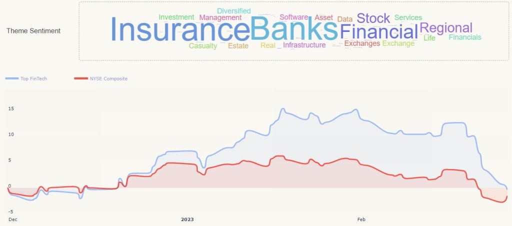
The Top FinTech investing theme is composed of its constituencies equally weighted against each other. The unweighted theme is a starting point to create an optimal asset allocation strategy. Asset allocation is one of the essential concepts in investing that is directly related to the way most investors balance their risk and return expectations. However, the asset allocation that works best for you at any given point in your life will depend primarily on your current time horizon and your ability to tolerate risk. Even though as time goes on, your portfolio asset allocation will drift away from your preferred positions in Top FinTech, you can continually rebalance it towards the optimal future performance using our optimization engine.

Top FinTech theme market capitalization (MC) usually refers to the total value of a theme’s positions broken down into specific market cap categories. To manage market risk and economic uncertainty, many investors today build portfolios that are diversified across equities with different market capitalizations. However, as a general rule, conservative investors tend to hold large-cap stocks, and these looking for more risk prefer small-cap and mid-cap equities:

Large MC 85%, Mid MC 15%.

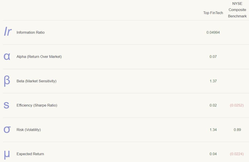
The market elasticity of a theme is the measure of how responsive the resulted portfolio will be to changes in the market or economic conditions. Most investing themes are subject to two types of risk – systematic (i.e., market) and unsystematic (i.e., nonmarket or company-specific) risk. Unsystematic risk is the risk that events specific to Top FinTech theme will adversely affect the performance of its constituents. This type of risk can be diversified away by optimizing the themed equities into an efficient portfolio with different positions weighted according to their correlations. On the other hand, systematic risk is the risk that the theme constituents’ prices will be affected by overall market movements and cannot be diversified. Below are essential risk-adjusted performance indicators that can help to measure the overall market elasticity of the Top FinTech theme.

An investing theme such as Top FinTech should be diversified across asset classifications. So, in addition to allocating your investments among stocks, funds, ETFs, cash, and possibly cryptocurrencies, you will also need to spread out your investments within each asset category. The key is to identify investments in segments of each asset category that may perform differently under different market conditions. One way of diversifying your investments within an asset category is investing in a wide range of entities and industry sectors with different risk-return characteristics.

Many investors optimize their portfolios to maintain a risk-return balance that meets their personal investing preferences and liquidity needs. Understanding the relationship between the Sharpe ratio, risk, and expected return will help you build an optimal portfolio out of your selected theme. The Sharpe ratios describe how much excess return you receive for the extra volatility you endure for holding a position in a themed portfolio. Below are the essential efficiency ratios that can help you quickly create a reliable input to your portfolio optimization process.

TradingView Community

TradingView chart SPDR S&P Regional Banking ETF

A lot of talk on who is to blame for the SVB Financial collapse – this is the first big casualty of rapid rate hikes and tighter policy, but who is to blame and what are the next steps?

-SVBs management – they invested short-term deposits in longer term fixed income assets – where a large % of its $120b securities portfolio lacked any kind of interest rate hedge (payers swaps were clearly needed)

-SVBs management – In the past 8 months SVB had no risk manager – fortune.com/2023/03/…-chief-risk-officer/ – no one knows how they efficiently managed risk

-SVBs management – the accounts showed they held $91b of its $120b securities in its HTM (assets Held to Maturity) book – these are assets they intend to hold until maturity but the accounting rules detail, that they don’t need to mark-to-market the moves in the underlying and report the ballooning losses – which again were not hedged.

-SVB deposit mix – 93%+ were above the FDIC insurance limit – this makes depositors v sensitive to any capital concerns at the bank

-SVB deposit mix – VCs had a rapid cash burn, as projects they back are typically driven by changes in interest rates (think Net Present value and Internal rates of return) – depositors took cash off SVB’s balance sheet to fund operations – SVB subsequently had to sell assets as their liabilities fell – we then see realised losses from buying securities at much higher prices.

-Short sellers/investor base – shorts had an eye on unrealised losses from the worsening asset quality for weeks – the selling accelerated when the CEO/ CFO /CMO disclosed they’d sold a chunk of stock on 27 March – it was over when the SVB took a $1.8b hit on its AFS securities available for sale on Wednesday – management sold $21b of its $28b book and announced a $2.25b in equity/debt raising – investors knew with conviction that depositors were fleeing – who supports a raising when liabilities are falling – no one sensible, raising pulled

-The Fed – failing to know such a shift in rates would impact banks asset quality when its primary function is financial stability.

-Regulation – Basel 3 – banks being forced to buy govt paper against deposits – v low risk weighting (perhaps required a hedge

Hard to pinpoint this on one aspect IMO – I think there is a perfect storm going on – a lack of hedging of interest rate risk was clearly a dominant factor behind this. Top down this is a function of rapidly tightening monetary policy and the impact this had on both the asset quality and liability side of the balance sheet – we should recall SVBs model is not the same as others in the banking space, so its hard to say this is systemic – still we wait for the outcome on next steps on how deposits over $250k will be dealt with – we’re hearing they may get 50% back initially but a buyer would be the best solution

The issue for regional/smaller banks comes if is we see some sort of haircut on the deposits claim over $250k – that could see a loss of confidence in holding deposits with other smaller banks names – we shall hear more soon, but broad contagion through the financial system seems unlikely, but it is a possibility given nearly 1/3 deposits in the banking system are uninsured – any bank with a large asset base and low equity are in the spotlight

As said Friday this could be a nothing burger or have real impactions on economics – the big issue happens this week if we see no clarity on how depositors are dealt (seems unlikely) with and we get a hot CPI print

TradingView BAC price chart BB and Stoch oscillator

Bank of America peaked February 2022 and last month produced a year long lower high.
✔️ This week BAC produced the highest selling volume since June 2020.
✔️ BAC closed Friday below MA200 and EMA300 in a single candle.
✔️ It was already trading below EMA50, EMA100, etc.
✔️ The MACD did a bearish cross while moving below zero… Double whammy.
✔️ The RSI is already weak and gaining bearish momentum.

TradingView BAC Summary 1 week Strong Sell

Barchart Platform

BAC 6-month price vs $NYA (blue curve).

Trading Indicators

let’s set the working directory

import os
os.chdir(‘YOURPATH’)
os. getcwd()

and get the BAC data since 2023-01-01

import pandas as pd
import numpy as np
import requests
import matplotlib.pyplot as plt
from math import floor
from termcolor import colored as cl

plt.style.use(‘fivethirtyeight’)
plt.rcParams[‘figure.figsize’] = (20,10)

def get_historical_data(symbol, start_date):
api_key = ‘your_api_key’
api_url = f’https://api.twelvedata.com/time_series?symbol={symbol}&interval=1day&outputsize=5000&apikey={api_key}’
raw_df = requests.get(api_url).json()
df = pd.DataFrame(raw_df[‘values’]).iloc[::-1].set_index(‘datetime’).astype(float)
df = df[df.index >= start_date]
df.index = pd.to_datetime(df.index)
return df

aapl = get_historical_data(‘BAC’, ‘2023-01-01’)

Let’s plot the BAC closing price, DI, ADX 14 indicators and trading signals

def get_adx(high, low, close, lookback):
plus_dm = high.diff()
minus_dm = low.diff()
plus_dm[plus_dm < 0] = 0 minus_dm[minus_dm > 0] = 0

tr1 = pd.DataFrame(high - low)
tr2 = pd.DataFrame(abs(high - close.shift(1)))
tr3 = pd.DataFrame(abs(low - close.shift(1)))
frames = [tr1, tr2, tr3]
tr = pd.concat(frames, axis = 1, join = 'inner').max(axis = 1)
atr = tr.rolling(lookback).mean()

plus_di = 100 * (plus_dm.ewm(alpha = 1/lookback).mean() / atr)
minus_di = abs(100 * (minus_dm.ewm(alpha = 1/lookback).mean() / atr))
dx = (abs(plus_di - minus_di) / abs(plus_di + minus_di)) * 100
adx = ((dx.shift(1) * (lookback - 1)) + dx) / lookback
adx_smooth = adx.ewm(alpha = 1/lookback).mean()
return plus_di, minus_di, adx_smooth

aapl[‘plus_di’] = pd.DataFrame(get_adx(aapl[‘high’], aapl[‘low’], aapl[‘close’], 14)[0]).rename(columns = {0:’plus_di’})
aapl[‘minus_di’] = pd.DataFrame(get_adx(aapl[‘high’], aapl[‘low’], aapl[‘close’], 14)[1]).rename(columns = {0:’minus_di’})
aapl[‘adx’] = pd.DataFrame(get_adx(aapl[‘high’], aapl[‘low’], aapl[‘close’], 14)[2]).rename(columns = {0:’adx’})
aapl = aapl.dropna()
aapl.tail()

ax1 = plt.subplot2grid((11,1), (0,0), rowspan = 5, colspan = 1)
ax2 = plt.subplot2grid((11,1), (6,0), rowspan = 5, colspan = 1)
ax1.plot(aapl[‘close’], linewidth = 2, color = ‘#ff9800’)
ax1.set_title(‘BAC CLOSING PRICE’)
ax2.plot(aapl[‘plus_di’], color = ‘#26a69a’, label = ‘+ DI 14’, linewidth = 3, alpha = 0.3)
ax2.plot(aapl[‘minus_di’], color = ‘#f44336’, label = ‘- DI 14’, linewidth = 3, alpha = 0.3)
ax2.plot(aapl[‘adx’], color = ‘#2196f3’, label = ‘ADX 14’, linewidth = 3)
ax2.axhline(25, color = ‘grey’, linewidth = 2, linestyle = ‘–‘)
ax2.legend()
ax2.set_title(‘BAC ADX 14’)
plt.show()

def implement_adx_strategy(prices, pdi, ndi, adx):
buy_price = []
sell_price = []
adx_signal = []
signal = 0

for i in range(len(prices)):
    if adx[i-1] < 25 and adx[i] > 25 and pdi[i] > ndi[i]:
        if signal != 1:
            buy_price.append(prices[i])
            sell_price.append(np.nan)
            signal = 1
            adx_signal.append(signal)
        else:
            buy_price.append(np.nan)
            sell_price.append(np.nan)
            adx_signal.append(0)
    elif adx[i-1] < 25 and adx[i] > 25 and ndi[i] > pdi[i]:
        if signal != -1:
            buy_price.append(np.nan)
            sell_price.append(prices[i])
            signal = -1
            adx_signal.append(signal)
        else:
            buy_price.append(np.nan)
            sell_price.append(np.nan)
            adx_signal.append(0)
    else:
        buy_price.append(np.nan)
        sell_price.append(np.nan)
        adx_signal.append(0)

return buy_price, sell_price, adx_signal

buy_price, sell_price, adx_signal = implement_adx_strategy(aapl[‘close’], aapl[‘plus_di’], aapl[‘minus_di’], aapl[‘adx’])

ax1 = plt.subplot2grid((11,1), (0,0), rowspan = 5, colspan = 1)
ax2 = plt.subplot2grid((11,1), (6,0), rowspan = 5, colspan = 1)
ax1.plot(aapl[‘close’], linewidth = 3, color = ‘#ff9800’, alpha = 0.6)
ax1.set_title(‘BAC CLOSING PRICE’)
ax1.plot(aapl.index, buy_price, marker = ‘^’, color = ‘#26a69a’, markersize = 14, linewidth = 0, label = ‘BUY SIGNAL’)
ax1.plot(aapl.index, sell_price, marker = ‘v’, color = ‘#f44336’, markersize = 14, linewidth = 0, label = ‘SELL SIGNAL’)
ax2.plot(aapl[‘plus_di’], color = ‘#26a69a’, label = ‘+ DI 14’, linewidth = 3, alpha = 0.3)
ax2.plot(aapl[‘minus_di’], color = ‘#f44336’, label = ‘- DI 14’, linewidth = 3, alpha = 0.3)
ax2.plot(aapl[‘adx’], color = ‘#2196f3’, label = ‘ADX 14’, linewidth = 3)
ax2.axhline(25, color = ‘grey’, linewidth = 2, linestyle = ‘–‘)
ax2.legend()
ax2.set_title(‘BAC ADX 14’)
plt.show()

BAC closing price, ADX 14 and trading signals

Let’s define our position

position = []
for i in range(len(adx_signal)):
if adx_signal[i] > 1:
position.append(0)
else:
position.append(1)

for i in range(len(aapl[‘close’])):
if adx_signal[i] == 1:
position[i] = 1
elif adx_signal[i] == -1:
position[i] = 0
else:
position[i] = position[i-1]

close_price = aapl[‘close’]
plus_di = aapl[‘plus_di’]
minus_di = aapl[‘minus_di’]
adx = aapl[‘adx’]
adx_signal = pd.DataFrame(adx_signal).rename(columns = {0:’adx_signal’}).set_index(aapl.index)
position = pd.DataFrame(position).rename(columns = {0:’adx_position’}).set_index(aapl.index)

frames = [close_price, plus_di, minus_di, adx, adx_signal, position]
strategy = pd.concat(frames, join = ‘inner’, axis = 1)

strategy

Let’s check our daily returns

rets = aapl.close.pct_change().dropna()
strat_rets = strategy.adx_position[1:]*rets

plt.title(‘Daily Returns’)
rets.plot(color = ‘blue’, alpha = 0.3, linewidth = 7)
strat_rets.plot(color = ‘r’, linewidth = 1)
plt.show()

rets_cum = (1 + rets).cumprod() – 1
strat_cum = (1 + strat_rets).cumprod() – 1

plt.title(‘Cumulative Returns’)
rets_cum.plot(color = ‘blue’, alpha = 0.3, linewidth = 7)
strat_cum.plot(color = ‘r’, linewidth = 2)
plt.show()

ADX Strategy Backtesting

Let’s check the expected profit by investing $10k in BAC

aapl_ret = pd.DataFrame(np.diff(aapl[‘close’])).rename(columns = {0:’returns’})
adx_strategy_ret = []

for i in range(len(aapl_ret)):
returns = aapl_ret[‘returns’][i]*strategy[‘adx_position’][i]
adx_strategy_ret.append(returns)

adx_strategy_ret_df = pd.DataFrame(adx_strategy_ret).rename(columns = {0:’adx_returns’})
investment_value = 10000
number_of_stocks = floor(investment_value/aapl[‘close’][-1])
adx_investment_ret = []

for i in range(len(adx_strategy_ret_df[‘adx_returns’])):
returns = number_of_stocks*adx_strategy_ret_df[‘adx_returns’][i]
adx_investment_ret.append(returns)

adx_investment_ret_df = pd.DataFrame(adx_investment_ret).rename(columns = {0:’investment_returns’})
total_investment_ret = round(sum(adx_investment_ret_df[‘investment_returns’]), 2)
profit_percentage = floor((total_investment_ret/investment_value)*100)
print(cl(‘Profit gained from the ADX strategy by investing $10k in BAC : {}’.format(total_investment_ret), attrs = [‘bold’]))
print(cl(‘Profit percentage of the ADX strategy : {}%’.format(profit_percentage), attrs = [‘bold’]))

Profit gained from the ADX strategy by investing $10k in BAC : -2127.06
Profit percentage of the ADX strategy : -22%

Let’s check the expected profit by investing $10k in $SPY (benchmark)

def get_benchmark(start_date, investment_value):
spy = get_historical_data(‘SPY’, start_date)[‘close’]
benchmark = pd.DataFrame(np.diff(spy)).rename(columns = {0:’benchmark_returns’})

investment_value = investment_value
number_of_stocks = floor(investment_value/spy[-1])
benchmark_investment_ret = []

for i in range(len(benchmark['benchmark_returns'])):
    returns = number_of_stocks*benchmark['benchmark_returns'][i]
    benchmark_investment_ret.append(returns)

benchmark_investment_ret_df = pd.DataFrame(benchmark_investment_ret).rename(columns = {0:'investment_returns'})
return benchmark_investment_ret_df

benchmark = get_benchmark(‘2023-01-01’, 10000)

investment_value = 10000
total_benchmark_investment_ret = round(sum(benchmark[‘investment_returns’]), 2)
benchmark_profit_percentage = floor((total_benchmark_investment_ret/investment_value)*100)
print(cl(‘Benchmark profit by investing $10k : {}’.format(total_benchmark_investment_ret), attrs = [‘bold’]))
print(cl(‘Benchmark Profit percentage : {}%’.format(benchmark_profit_percentage), attrs = [‘bold’]))
print(cl(‘ADX Strategy profit is {}% higher than the Benchmark Profit’.format(profit_percentage – benchmark_profit_percentage), attrs = [‘bold’]))

Benchmark profit by investing $10k : 201.25
Benchmark Profit percentage : 2%
ADX Strategy profit is -24% higher than the Benchmark Profit

Risk-Return Optimization

Download multiple assets history:

import yfinance as yf
import pandas as pd
import numpy as np
import matplotlib.pyplot as plt

def download(tickers, start=None, end=None, actions=False, threads=True,
group_by=’column’, auto_adjust=False, back_adjust=False,
progress=True, period=”max”, show_errors=True, interval=”1d”, prepost=False,
proxy=None, rounding=False, timeout=None, **kwargs):

benchmark_ = [“^GSPC”,]
portfolio_ = [‘BAC’, ‘PGR’, ‘JPM’, ‘AXP’, ‘HCP’, ‘BEN’, ‘COF’, ‘CINF’, ‘C’, ‘MCO’, ‘PLD’, ‘BK’, ‘GNW’, ‘VTR’, ‘ESS’, ‘DFS’,’NTRS’, ‘UNM’, ‘MS’, ‘TROW’]

start_date_ = “2023-01-01”
end_date_ = “2023-03-15”
number_of_scenarios = 10000

return_vector = []
risk_vector = []
distrib_vector = []

df = yf.download(benchmark_, start=start_date_, end=end_date_)
df2 = yf.download(portfolio_, start=start_date_, end=end_date_)

df = df.dropna(axis=0)
df2 = df2.dropna(axis=0)

df = df[df.index.isin(df2.index)]

[*********************100%***********************]  1 of 1 completed
[*********************100%***********************]  20 of 20 completed

Analysis of Benchmark:

benchmark_vector = np.array(df[‘Close’])

benchmark_vector = np.diff(benchmark_vector)/benchmark_vector[1:]

benchmark_return = np.average(benchmark_vector)
benchmark_risk = np.std(benchmark_vector)

return_vector.append(benchmark_return)
risk_vector.append(benchmark_risk)

Analysis of Portfolio:
portfolio_vector = np.array(df2[‘Close’])

Create a loop for the number of scenarios we want:

for i in range(number_of_scenarios):
#Create a random distribution that sums 1
# and is split by the number of stocks in the portfolio
random_distribution = np.random.dirichlet(np.ones(len(portfolio_)),size=1)
distrib_vector.append(random_distribution)

#Find the Closing Price for everyday of the portfolio
portfolio_matmul = np.matmul(random_distribution,portfolio_vector.T)

#Calculate the daily return
portfolio_matmul = np.diff(portfolio_matmul)/portfolio_matmul[:,1:]

#Select or Final Return and Risk
portfolio_return = np.average(portfolio_matmul, axis=1)
portfolio_risk = np.std(portfolio_matmul, axis=1)

#Add our Benchmark info to our lists
return_vector.append(portfolio_return[0])
risk_vector.append(portfolio_risk[0])

Create Risk Boundaries
delta_risk = 0.1
min_risk = np.min(risk_vector)
max_risk = risk_vector[0]*(1+delta_risk)
risk_gap = [min_risk, max_risk]

Portfolio Return and Risk Couple
portfolio_array = np.column_stack((return_vector,risk_vector))[1:,]

Rule to create the best portfolio:

if np.where(((portfolio_array[:,1]<= max_risk)))[0].shape[0]>1:
min_risk_portfolio = np.where(((portfolio_array[:,1]<= max_risk)))[0]
best_portfolio_loc = portfolio_array[min_risk_portfolio]
max_loc = np.argmax(best_portfolio_loc[:,0])
best_portfolio = best_portfolio_loc[max_loc]

else:
min_risk_portfolio = np.where(((portfolio_array[:,1]== np.min(risk_vector[1:]))))[0]
best_portfolio_loc = portfolio_array[min_risk_portfolio]
max_loc = np.argmax(best_portfolio_loc[:,0])
best_portfolio = best_portfolio_loc[max_loc]

Visual Representation

trade_days_per_year = 252
risk_gap = np.array(risk_gap)trade_days_per_year best_portfolio[0] = np.array(best_portfolio[0])trade_days_per_year
x = np.array(risk_vector)
y = np.array(return_vector)*trade_days_per_year

fig, ax = plt.subplots(figsize=(20, 15))

plt.rc(‘axes’, titlesize=14) # Controls Axes Title
plt.rc(‘axes’, labelsize=14) # Controls Axes Labels
plt.rc(‘xtick’, labelsize=14) # Controls x Tick Labels
plt.rc(‘ytick’, labelsize=14) # Controls y Tick Labels
plt.rc(‘legend’, fontsize=14) # Controls Legend Font
plt.rc(‘figure’, titlesize=14) # Controls Figure Title

ax.scatter(x, y, alpha=0.5,
linewidths=0.1,
edgecolors=’black’,
label=’Portfolio Scenarios’
)

ax.scatter(x[0],
y[0],
color=’red’,
linewidths=1,
edgecolors=’black’,
label=’Market Proxy Values’)

ax.scatter(best_portfolio[1],
best_portfolio[0],
color=’green’,
linewidths=1,
edgecolors=’black’,
label=’Best Performer’)

ax.axvspan(min_risk,
max_risk,
color=’red’,
alpha=0.08,
label=’Accepted Risk Zone’)

ax.set_ylabel(“Yearly Portfolio Average Return (%)”,fontsize=14)
ax.set_xlabel(“Yearly Portfolio Standard Deviation”,fontsize=14)

ax.axhline(y=0, color=’black’,alpha=0.5)

ax = plt.gca()
ax.legend(loc=0)
vals = ax.get_yticks()
ax.set_yticklabels([‘{:,.2%}’.format(x) for x in vals])

plt.savefig(‘risk_optimizer.png’, dpi=300)

BAC Price Prediction

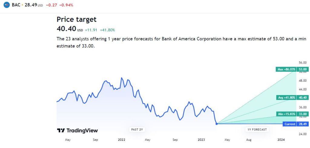
TradingView BAC 1Y forecast

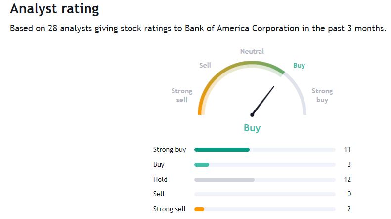
TradingView BAC analyst rating

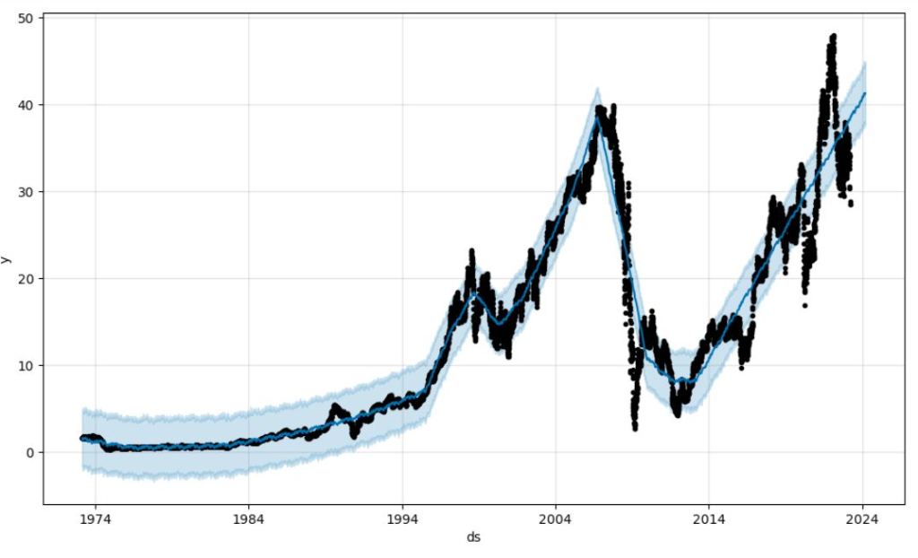
Prophet forecast: BAC price

Prophet forecast: BAC trend

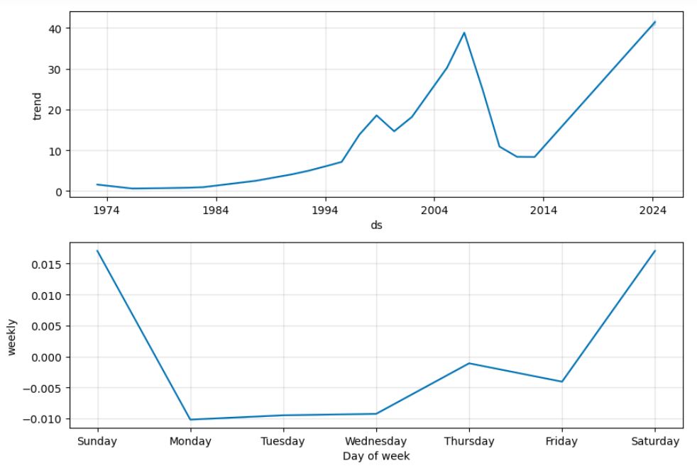
Prophet forecast: BAC seasonality

Summary

Guardian Headlines: Governments and regulators around the world, including in the UK and Australia, are checking for SVB exposure in their corporate and banking sectors.
Most forecasters expect rates to go higher in the US, UK and Australia, before stabilising.
The appetite to keep raising rates will now be tested if central banks become concerned that SVB’s problems are indicative of a broader weakness in corporate balance sheets caused by rising rates.
SeekingAlpha Courage & Conviction Investing said the SVB blow-up is a good prompt for retirees, who are invested in high dividend-yielding stocks, to re-examine the amount of risk they are taking. Contributor Ian Bezek said the collapse shows the issue of putting too many eggs in one basket, with respect to fixed income securities.
Zacks analysis: for investors in potentially troubled banks, there’s no relief coming for them if those banks got into a bind, hence the extra volatility. And likely continued volatility for those on the downgrade bubble.
Swiss Life Asset Managers – best practices of asset risk management strategies
Example Macroaxis risk-aware investment portfolio – Top FinTech theme explained and revised after SVB collapse
TradingView: BAC 1 week summary STRONG SELL, SVBs management – they invested short-term deposits in longer term fixed income assets – where a large % of its $120b securities portfolio lacked any kind of interest rate hedge
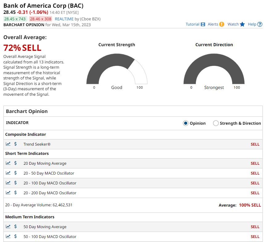
Barchart Opinion: 72% SELL BAC (3-day measurement, 13 trading indicators)
BAC data since 2023-01-01 to test ADX-14 strategy – 1 BUY and 1 SELL signals.
Profit gained from the ADX strategy by investing $10k in BAC : -2127.06 Profit percentage of the ADX strategy : -22%
Benchmark profit by investing $10k : 201.25
Benchmark Profit percentage : 2%
ADX Strategy profit is -24% higher than the Benchmark Profit
Example Risk/Return Portfolio Optimization 2023 32% return & 0.01 STDV: benchmark_ = [“^GSPC”,]
portfolio_ = [‘BAC’, ‘PGR’, ‘JPM’, ‘AXP’, ‘HCP’, ‘BEN’, ‘COF’, ‘CINF’, ‘C’, ‘MCO’, ‘PLD’, ‘BK’, ‘GNW’, ‘VTR’, ‘ESS’, ‘DFS’,’NTRS’, ‘UNM’, ‘MS’, ‘TROW’]
start_date_ = “2023-01-01”
end_date_ = “2023-03-15”
number_of_scenarios = 10000, Risk Boundaries delta_risk = 0.1
BAC trend: FB Prophet 1Y forecast is consistent with the TradingView analyst rating and price prediction.

Explore More

A Comparative Analysis of The 3 Best U.S. Growth Stocks in Q1’23 – 3. LYTS

Make a one-time donation

Make a monthly donation

Make a yearly donation

Choose an amount

€5.00

€15.00

€100.00

€5.00

€15.00

€100.00

€5.00

€15.00

€100.00

Or enter a custom amount

€

Your contribution is appreciated.

Donate Donate monthly Donate yearly

Post-SVB Risk Aware Investing

Headlines

Seeking Alpha Update

Zacks Investment Research

Swiss Life Asset Managers

Macroaxis Wealth Optimization

TradingView Community

Barchart Platform

Trading Indicators

ADX Strategy Backtesting

Risk-Return Optimization

BAC Price Prediction

Summary

Explore More

Make a one-time donation

Make a monthly donation

Make a yearly donation

Share this:

Leave a comment Cancel reply