BTC-USD Price Prediction with LSTM

Some experts call Bitcoin “the currency of the future”. The Bitcoin price has increased several times during the 2017 year. At the same time, it is very volatile.

The objective of this project is to test the deep learning algorithm of real-time BTC-USD price prediction in Q4 ’22.

The entire Python workflow looks like this:

• Importing the necessary Python libraries
• Load and check the real-time input dataset
• Data editing, transformations and preparations
• Exploratory Data Analysis (EDA)
• Training 2-layers LSTM Neural Network (NN)
• Check Predicted vs Actual Prices USD + RMSE

Let’s set the working directory YOURPATH

import os
os.chdir(‘YOURPATH’) # Set working directory
os. getcwd()

and import the libraries

import warnings
warnings.filterwarnings(“ignore”)

import numpy as np
import pandas as pd
import statsmodels.api as sm
from scipy import stats
from sklearn.metrics import mean_squared_error
from math import sqrt
from random import randint
from keras.models import Sequential
from keras.layers import Dense
from keras.layers import LSTM
from keras.layers import GRU
from keras.callbacks import EarlyStopping
from keras import initializers
from matplotlib import pyplot
from datetime import datetime
from matplotlib import pyplot as plt
import plotly.offline as py
import plotly.graph_objs as go
py.init_notebook_mode(connected=True)
%matplotlib inline

import yfinance as yf
import datetime
from datetime import date, timedelta

Let’s load the input real-time dataset

today = date.today()

d1 = today.strftime(“%Y-%m-%d”)
end_date = d1
d2 = date.today() – timedelta(days=730)
d2 = d2.strftime(“%Y-%m-%d”)
start_date = d2

data = yf.download(‘BTC-USD’,
start=start_date,
end=end_date,
progress=False)
data[“Date”] = data.index
data = data[[“Date”, “Open”, “High”, “Low”, “Close”, “Adj Close”, “Volume”]]
data.reset_index(drop=True, inplace=True)
print(data.tail())

Date          Open          High           Low         Close  \
725 2022-10-21  19053.203125  19237.384766  18770.970703  19172.468750   
726 2022-10-22  19172.380859  19248.068359  19132.244141  19208.189453   
727 2022-10-23  19207.734375  19646.652344  19124.197266  19567.007812   
728 2022-10-24  19567.769531  19589.125000  19206.324219  19345.572266   
729 2022-10-25  19344.964844  20348.412109  19261.447266  20095.857422   

        Adj Close       Volume  
725  19172.468750  32459287866  
726  19208.189453  16104440957  
727  19567.007812  22128794335  
728  19345.572266  30202235805  
729  20095.857422  47761524910

and check the content

data.shape

(730, 7)

data.info()

<class 'pandas.core.frame.DataFrame'>
RangeIndex: 730 entries, 0 to 729
Data columns (total 7 columns):
 #   Column     Non-Null Count  Dtype         
---  ------     --------------  -----         
 0   Date       730 non-null    datetime64[ns]
 1   Open       730 non-null    float64       
 2   High       730 non-null    float64       
 3   Low        730 non-null    float64       
 4   Close      730 non-null    float64       
 5   Adj Close  730 non-null    float64       
 6   Volume     730 non-null    int64         
dtypes: datetime64[ns](1), float64(5), int64(1)
memory usage: 40.0 KB

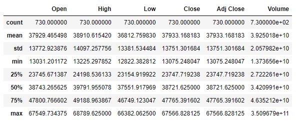
data.describe()

and check for the null/missing values

data.isnull().values.any()

False

Let’s group the Close price by the date

group = data.groupby(‘Date’)
Daily_Price = group[‘Close’].mean()

Daily_Price.tail()

Date
2022-10-21    19172.468750
2022-10-22    19208.189453
2022-10-23    19567.007812
2022-10-24    19345.572266
2022-10-25    20095.857422
Name: Close, dtype: float64

and create the time slots for training, testing and validation purposes

from datetime import date
d0 = date(2022, 1, 1)
d1 = date(2022, 10, 25)
delta = d1 – d0
days_look = delta.days + 1
print(days_look)

298

d0 = date(2022, 8, 25)
d1 = date(2022, 10, 25)
delta = d1 – d0
days_from_train = delta.days + 1
print(days_from_train)

62

d0 = date(2022, 10, 15)
d1 = date(2022, 10, 25)
delta = d1 – d0
days_from_end = delta.days + 1
print(days_from_end)

11

Let’s create the train and test data

df_train= Daily_Price[len(Daily_Price)-days_look-days_from_end:len(Daily_Price)-days_from_train]
df_test= Daily_Price[len(Daily_Price)-days_from_train:]

print(len(df_train), len(df_test))

247 62

Let’s concatenate these data

working_data = [df_train, df_test]
working_data = pd.concat(working_data)

working_data = working_data.reset_index()
working_data[‘Date’] = pd.to_datetime(working_data[‘Date’])
working_data = working_data.set_index(‘Date’)

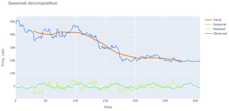
We are ready to apply sm.tsa.seasonal_decompose

s = sm.tsa.seasonal_decompose(working_data.Close.values,period=61)

and plot the result

trace1 = go.Scatter(x = np.arange(0, len(s.trend), 1),y = s.trend,mode = ‘lines’,name = ‘Trend’,
line = dict(color = (‘rgb(244, 146, 65)’), width = 4))
trace2 = go.Scatter(x = np.arange(0, len(s.seasonal), 1),y = s.seasonal,mode = ‘lines’,name = ‘Seasonal’,
line = dict(color = (‘rgb(66, 244, 155)’), width = 2))

trace3 = go.Scatter(x = np.arange(0, len(s.resid), 1),y = s.resid,mode = ‘lines’,name = ‘Residual’,
line = dict(color = (‘rgb(209, 244, 66)’), width = 2))

trace4 = go.Scatter(x = np.arange(0, len(s.observed), 1),y = s.observed,mode = ‘lines’,name = ‘Observed’,
line = dict(color = (‘rgb(66, 134, 244)’), width = 2))

data = [trace1, trace2, trace3, trace4]
layout = dict(title = ‘Seasonal decomposition’, xaxis = dict(title = ‘Time’), yaxis = dict(title = ‘Price, USD’))
fig = dict(data=data, layout=layout)
py.iplot(fig, filename=’seasonal_decomposition’)

We can plot autocorrelation

plt.figure(figsize=(15,7))
ax = plt.subplot(211)
sm.graphics.tsa.plot_acf(working_data.Close.values.squeeze(), lags=48, ax=ax)
ax = plt.subplot(212)
sm.graphics.tsa.plot_pacf(working_data.Close.values.squeeze(), lags=48, ax=ax)
plt.tight_layout()
plt.show()

Let’s look at the train and test data

df_train = working_data[:-61]
df_test = working_data[-61:]

and call the function

ef create_lookback(dataset, look_back=1):
X, Y = [], []
for i in range(len(dataset) – look_back):
a = dataset[i:(i + look_back), 0]
X.append(a)
Y.append(dataset[i + look_back, 0])
return np.array(X), np.array(Y)

Let’s prepare our data for ML

from sklearn.preprocessing import RobustScaler

training_set = df_train.values
training_set = np.reshape(training_set, (len(training_set), 1))
test_set = df_test.values
test_set = np.reshape(test_set, (len(test_set), 1))

Scale datasets:

scaler = RobustScaler()
training_set = scaler.fit_transform(training_set)
test_set = scaler.transform(test_set)

Create datasets which are suitable for time series forecasting

look_back = 1
X_train, Y_train = create_lookback(training_set, look_back)
X_test, Y_test = create_lookback(test_set, look_back)

# reshape datasets so that they will be ok for the requirements of the LSTM model in Keras
X_train = np.reshape(X_train, (len(X_train), 1, X_train.shape[1]))
X_test = np.reshape(X_test, (len(X_test), 1, X_test.shape[1]))

Let’s create our trained model

Initialize sequential model, add 2 stacked LSTM layers and densely connected output neuron

model = Sequential()
model.add(LSTM(256, return_sequences=True, input_shape=(X_train.shape[1], X_train.shape[2])))
model.add(LSTM(256))
model.add(Dense(1))

Compile and fit the NN model

model.compile(loss=’mean_squared_error’, optimizer=’adam’)
history = model.fit(X_train, Y_train, epochs=100, batch_size=16, shuffle=False,
validation_data=(X_test, Y_test),
callbacks = [EarlyStopping(monitor=’val_loss’, min_delta=5e-5, patience=20, verbose=1)])

Epoch 1/100
16/16 [==============================] - 3s 42ms/step - loss: 0.2524 - val_loss: 0.6315
Epoch 2/100
16/16 [==============================] - 0s 7ms/step - loss: 0.0893 - val_loss: 0.0899
Epoch 3/100
16/16 [==============================] - 0s 6ms/step - loss: 0.0289 - val_loss: 0.0048
Epoch 4/100
16/16 [==============================] - 0s 6ms/step - loss: 0.0079 - val_loss: 0.0016
Epoch 5/100
16/16 [==============================] - 0s 5ms/step - loss: 0.0050 - val_loss: 0.0016
Epoch 6/100
16/16 [==============================] - 0s 6ms/step - loss: 0.0047 - val_loss: 8.0767e-04
Epoch 7/100
16/16 [==============================] - 0s 6ms/step - loss: 0.0046 - val_loss: 8.8796e-04
Epoch 8/100
16/16 [==============================] - 0s 6ms/step - loss: 0.0049 - val_loss: 8.3084e-04
Epoch 9/100
16/16 [==============================] - 0s 6ms/step - loss: 0.0051 - val_loss: 8.0932e-04
Epoch 10/100
16/16 [==============================] - 0s 6ms/step - loss: 0.0061 - val_loss: 8.4507e-04
Epoch 11/100
16/16 [==============================] - 0s 6ms/step - loss: 0.0071 - val_loss: 0.0013
Epoch 12/100
16/16 [==============================] - 0s 6ms/step - loss: 0.0109 - val_loss: 8.1699e-04
Epoch 13/100
16/16 [==============================] - 0s 6ms/step - loss: 0.0133 - val_loss: 0.0031
Epoch 14/100
16/16 [==============================] - 0s 6ms/step - loss: 0.0244 - val_loss: 0.0075
Epoch 15/100
16/16 [==============================] - 0s 6ms/step - loss: 0.0196 - val_loss: 0.0016
Epoch 16/100
16/16 [==============================] - 0s 6ms/step - loss: 0.0299 - val_loss: 0.0226
Epoch 17/100
16/16 [==============================] - 0s 6ms/step - loss: 0.0136 - val_loss: 0.0010
Epoch 18/100
16/16 [==============================] - 0s 6ms/step - loss: 0.0145 - val_loss: 0.0094
Epoch 19/100
16/16 [==============================] - 0s 6ms/step - loss: 0.0084 - val_loss: 0.0010
Epoch 20/100
16/16 [==============================] - 0s 6ms/step - loss: 0.0085 - val_loss: 0.0039

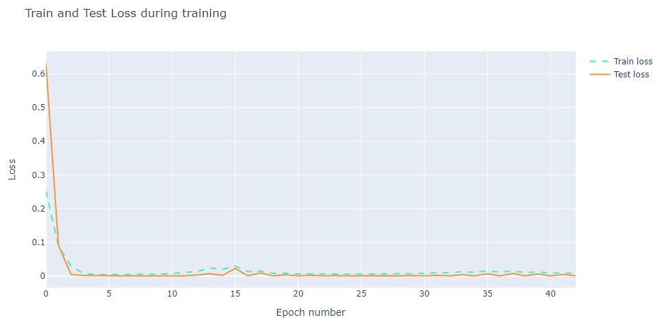
and plot the training process

trace1 = go.Scatter(
x = np.arange(0, len(history.history[‘loss’]), 1),
y = history.history[‘loss’],
mode = ‘lines’,
name = ‘Train loss’,
line = dict(color=(‘rgb(66, 244, 155)’), width=2, dash=’dash’)
)
trace2 = go.Scatter(
x = np.arange(0, len(history.history[‘val_loss’]), 1),
y = history.history[‘val_loss’],
mode = ‘lines’,
name = ‘Test loss’,
line = dict(color=(‘rgb(244, 146, 65)’), width=2)
)

data = [trace1, trace2]
layout = dict(title = ‘Train and Test Loss during training’,
xaxis = dict(title = ‘Epoch number’), yaxis = dict(title = ‘Loss’))
fig = dict(data=data, layout=layout)
py.iplot(fig, filename=’training_process’)

Let’s get predictions and then make some transformations to be able to calculate RMSE properly in USD
prediction = model.predict(X_test)
prediction_inverse = scaler.inverse_transform(prediction.reshape(-1, 1))
Y_test_inverse = scaler.inverse_transform(Y_test.reshape(-1, 1))
prediction2_inverse = np.array(prediction_inverse[:,0][1:])
Y_test2_inverse = np.array(Y_test_inverse[:,0])

2/2 [==============================] - 0s 2ms/step

The resulting plot is

trace1 = go.Scatter(
x = np.arange(0, len(prediction2_inverse), 1),
y = prediction2_inverse,
mode = ‘lines’,
name = ‘Predicted price’,
hoverlabel= dict(namelength=-1),
line = dict(color=(‘rgb(244, 146, 65)’), width=2)
)
trace2 = go.Scatter(
x = np.arange(0, len(Y_test2_inverse), 1),
y = Y_test2_inverse,
mode = ‘lines’,
name = ‘True price’,
line = dict(color=(‘rgb(66, 244, 155)’), width=2)
)

data = [trace1, trace2]
layout = dict(title = ‘Comparison of true prices (on the test dataset) with prices our model predicted’,
xaxis = dict(title = ‘Day number’), yaxis = dict(title = ‘Price, USD’))
fig = dict(data=data, layout=layout)
py.iplot(fig, filename=’results_demonstrating0′)

The RMSE is

RMSE = sqrt(mean_squared_error(Y_test2_inverse1, prediction2_inverse))
print(‘Test RMSE: %.3f’ % RMSE)

Test RMSE: 63.566

Let’s plot our BTC prices against the dates

Summary

• We trained the 2-layers Long Short Term Memory Neural Network using Bitcoin Historical Data.

• The trained LSTM model can be used to predict future price movements of bitcoin. 
• RMSE ~ $64, with the mean price of $20k (Oct ’22), which means the prediction error ~0.3%.
• The model performance is excellent, with an error of only tens of USD.

Explore More

Bitcoin price forecasting with deep learning algorithms

Cryptocurrency Price Prediction with Machine Learning