US Real Estate – Harnessing the Power of AI

This is the continuation of our recent use-case series dedicated to the real estate (RE) monitoring, trend analysis and forecast. In these series, the focus is on the US house prices by invoking supervised machine learning (ML) and artificial intelligence (AI) algorithms available in Python as it is the language with the largest variety of libraries on the subject (Scikit-learn, TensorFlow, pyTorch, Keras, SparkMLlib, etc.). Our objective is to incorporate these algorithms into the real estate decision making process thanks to its supporting role. Recall that decision-making is a critical part of a typical real estate property valuation aimed at quantifying the market value of a property according to its qualitative characteristics. Being visualization a prominent character of this kind of problems, ML/AI ETL pipelines are commonly used as a support for RE decision analysis. Within the context of testing and validation strategies, it is important to get into training errors and limitations of ML/AI due to its inherent pattern-recognizing nature.

ML/AI is defined as follows: A code learns from experience E with respect to a task T and a performance measure P, if its performance on T, as measured by P, improves with E. ML is a part of AI. ML algorithms build a model based on sample data, known as training data, in order to make predictions or decisions without being explicitly programmed to do so. ML is an important subset of data science. Through the use of statistical methods, data science algorithms are trained to make classifications or predictions, uncovering key insights within data mining projects. These insights subsequently drive decision making within applications and businesses, ideally impacting key BI/fintech metrics. 

Bottom Line: ML is the science of getting computers to learn, without being explicitly programmed.

Contents:

1. Housing Crunch
2. Content
3. Methodology
4. Prerequisites
5. Workflow
6. Case 1: US
7. Case 2: CA
8. Case 3: IA
   1. Let’s set the working directory YOURPATH
9. Case 4: MA
10. Crucial Steps
11. Key Takeaways
12. Conclusions
13. References

Housing Crunch

• The August 2022 NAHB measure of homebuilder confidence fell below 50 for the first time since May 2020. Housing starts for July dropped 9.6%, more than expected, (although permits dropped less than forecast). And most recently the NAR reported that July existing home sales fell 5.9%, more than anticipated.
• The August 2022 housing data did much to confirm a slowdown sought by the Federal Reserve. Along with what may have been peak inflation last week, cooler housing data is another piece in the puzzle as the FOMC tightens conditions.

• “Existing home sales have now fallen for 6 months in a row, and are 26% lower than the January 2022 peak,” Pantheon Macro Economist Ian Shepherdson said. “But the bottom is still some way off, given the degree to which demand has been crushed by rising rates; the required monthly mortgage payment for a new purchaser of an existing single-family home is no longer rising, but it was still up by 51% year-over-year in July 2022.
• “Home sales likely have further to fall,” Odeta Kushi, deputy chief economist at First American Financial, tweeted. “Mortgage applications so far in August 2022 point to another decline in existing-home sales. This month’s number of 4.81 million puts us at about 2014 sales level.”
• “Fed officials pay particularly close attention to the housing market and are monitoring how higher mortgage rates are impacting home sales and housing prices in order to gauge how tighter monetary policy is affecting the broader economy,” Wells Fargo economists wrote.

This post provides an optimized solution to the problem of unclear RE market changes by allowing brokerages and clients to have access to an ML-backed RE solution that draws upon different housing data sources that are updated to close recency.

Content

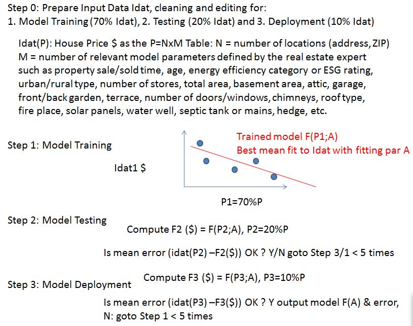
The paper is divided into the following sections: Business Case (see above), supervised ML Methodology, IDE and learning Prerequisites, ETL Python Workflow & Pipeline, multi-scale RE Use Cases using  comprehensive open-source housing datasets (US states and beyond), and Conclusions. Sections contain related links listed in References. Due to the scale of case studies, the entire ML project is split into several Jupyter notebooks: EDA and data cleaning, preprocessing and feature engineering, and model tuning and insights. Each input dataset is limited in scope both in terms of the time frame captured, as well as location. Each training model is also specific to houses in a city or county and may not be as accurate when applied to data from another US state, where house prices may be affected by different factors. The aim of specific training models is not to give a perfect prediction, but act as a guideline to inform RE decisions. In reality, house price may be difficult to predict as it is also affected by buyers’ psychology, the economic climate, and other factors not included in the dataset. 

Methodology

We consider the supervised ML techniques (see charts below) when we are given a (training) dataset and already know what our correct output should look like, providing the idea that there is an intrinsic relationship between the input and output data. In this study, house price prediction is regarded as a regression problem, meaning that we are trying to map input variables or features (the size of houses, area, etc.) to a continuous function (house price).

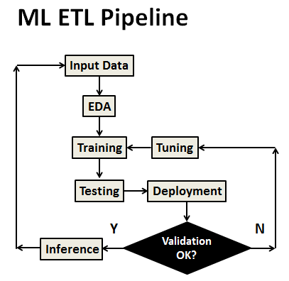
The supervised ML algorithm consists of the following steps:

• Create labeled data (label is the true answer for a given input, the house price $ is the label)
• Perform model training, testing and cross-validation
• Deploy trained models
• Evaluate and tune deployed models
• Avoid creating high bias/variance

Model training and evaluation is performed using chosen metrics and objectives. For example, the loss metric is a sum of squares between observed and predicted house prices.

The above three-step ML methodology is a way to use regression algorithms to derive predictive insights from housing data and make repeated RE decisions. Qualities of good data (output of EDA): it has coverage, is clean, is complete.

The broader your data’s coverage, the more robust your training model will be. Dirty data can make ML hard in terms of goodness-of-fit. Incomplete data can limit performance.

Here is the list of 10 popular ML regression algorithms:

1. Linear Regression
2. Ridge Regression
3. Neural Network Regression 
4. Lasso Regression 
5. Decision Tree Regression 
6. Random Forest
7. KNN Model 
8. Support Vector Machines (SVM)
9. Gausian Regression
10. Polynomial Regression

• Conventionally, the Exploratory Data Analysis (EDA) of the dataframe df is carried out using histograms df.plot(kind=’hist’) and pairplots sns.pairplot().

• The Feature Engineering (FE) phase consists of the following steps: Log Transform np.log() or Square Root Transform np.sqrt(), Feature Importance analysis coef_.ravel(), and Feature Scaling using StandardScaler() (most common option), RobustScaler() (not widely used option), and MinMaxScaler (least robust choice).
• The typical regression algorithm is the liner/polynomial regression with/without regularization (Lasso, Ridge, etc.) and/or Hyper-Parameter Optimization (HPO).
• The Model Evaluation phase may represent (optionally) the following comparisons: Ridge vs Lasso and Normal vs Polynomial.
• The cross-validation metrics utilities can be used to compute some useful statistics of the prediction performance. Some statistics computed are mean squared error (MSE), root mean squared error (RMSE), mean absolute error (MAE), mean absolute percent error (MAPE), and median absolute percent error (MDAPE). 

Prerequisites

We begin with setting up the Python-based IDE using the latest version of Anaconda that contains the Jupyter Noebook coupled with (optionally) Datapane. The latter allows you to share an html link in which you can layout your analysis as a report. When started, the Jupyter Notebook App can access only files within its start-up folder (including any sub-folder). No configuration is necessary if you place your notebooks in your home folder or subfolders. Otherwise, you need to choose a Jupyter Notebook App start-up folder which will contain all the notebooks. Read more here.

Check ML learning prerequisites here.

Workflow

The general workflow to create the model will be as follows:

• Data handling (loading, cleaning, editing or preprocessing)

• Exploratory Data Analysis (EDA)/Feature Engineering (FE)

We use Feature Engineering to deal with missing values, outliers, and categorical features

• Model training & hyperparameter tuning

We use various ML models and train/test them on train/test data, viz. after tuning all the hyperparameters, test the model on test data

• Model testing, QC diagnostics, evaluation and final deployment

• Apply predictions, result interpretation, visualization and export.

Below is the more detailed sequence of steps:

• Import Libraries and Loading Dataset

Example: use Python, opendatasets to load the data from the Kaggle platform, pandas to read and manipulate the data, seaborn, matplotlib, plotly, geopandas for data points visualizations, sklearn for data preprocessing and training algorithms.

• EDA & Data Visualization/Overview

Use a variety of useful data visualization tools that we can analyze tabular data and discover data cleaning procedures that we can fix the data (e.g. looking for missing values and outliers, applying data cleaning by removing unnecessary values or columns, duplicates values, and fixing some errors which can be human-made mistakes when recording).

• Feature Engineering & Selection to improve a model’s predictive performance

Use feature selection techniques such as Feature Importance (using ML algorithms such as Lasso and Random Forest), Correlation Matrix with Heatmap, or Univariate Selection. For example, we may choose the Heatmap correlation matrix technique to select features with correlations higher than zero.

• Data preparation/preprocessing using features scaling, encoding, and imputing

For example, the function preprocess_data(data) consists of remove_duplicates(), check_missing(), resolve_missing(), and change_types(); it takes in raw data and converts it into data that is ready for making predictions. Here are the steps to be done: 

Identify the input and target column(s) for training the model.

Identify numeric and categorical input columns.

Impute (fill) missing values in numeric columns

Scale values in numeric columns to a (0,1) range.

Encode categorical data into one-hot vectors.

Split the dataset into training and validation sets.

• Robust model training and hyperparameter tuning

For example, We may decide to train the data on SkLearn models Random Forest, Gradient Boosting, ExtraTree, LightGBM, and Catboost.

The predictions from the model can be evaluated using a loss function like the Root Mean Squared Error (RMSE).

• We can use the trained model to generate predictions for the training, testing and validation inputs by calculating the R-square in each case. The final score can be the model score and the training/testing accuracy.

Case 1: US

Let’s set the working directory YOURPATH

import os
os.chdir(‘YOURPATH’)
os. getcwd()

and import the following libraries

import pandas as pd
import numpy as np
import seaborn as sns
import matplotlib.pyplot as plt

from sklearn.model_selection import train_test_split

from sklearn.linear_model import LinearRegression

Let’s read the Kaggle dataset

houseDF = pd.read_csv(‘USA_Housing.csv’)

and check the file content

houseDF.shape

(5000, 7)

houseDF.columns

Index(['Avg. Area Income', 'Avg. Area House Age', 'Avg. Area Number of Rooms',
       'Avg. Area Number of Bedrooms', 'Area Population', 'Price', 'Address'],
      dtype='object')

houseDF.dtypes

Avg. Area Income                float64
Avg. Area House Age             float64
Avg. Area Number of Rooms       float64
Avg. Area Number of Bedrooms    float64
Area Population                 float64
Price                           float64
Address                          object
dtype: object

The info is

houseDF.info()

<class 'pandas.core.frame.DataFrame'>
RangeIndex: 5000 entries, 0 to 4999
Data columns (total 7 columns):
 #   Column                        Non-Null Count  Dtype  
---  ------                        --------------  -----  
 0   Avg. Area Income              5000 non-null   float64
 1   Avg. Area House Age           5000 non-null   float64
 2   Avg. Area Number of Rooms     5000 non-null   float64
 3   Avg. Area Number of Bedrooms  5000 non-null   float64
 4   Area Population               5000 non-null   float64
 5   Price                         5000 non-null   float64
 6   Address                       5000 non-null   object 
dtypes: float64(6), object(1)
memory usage: 273.6+ KB

and the first 5 rows are

houseDF.head(5)

while the input data descriptive statistics is

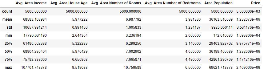
The input data pairplot is

fig=sns.pairplot(houseDF)
fig.savefig(“pairplot.png”)

and the correlation heatmap is

swarm_plot=sns.heatmap(houseDF.corr(), annot=True)
fig = swarm_plot.get_figure()
fig.savefig(“corrplot.png”)

Let’s separate features and target variables

X = houseDF[[‘Avg. Area Income’, ‘Avg. Area House Age’ , ‘Avg. Area Number of Rooms’, ‘Avg. Area Number of Bedrooms’, ‘Area Population’]]

Y = houseDF[‘Price’]

Let’s split the data into the train and test subsets as 70:30%, respectively,

from sklearn.model_selection import train_test_split
X_train, X_test, Y_train, Y_test= train_test_split(X,Y,test_size=0.30, random_state=1)

Let’s apply the LinearRegression() to the training data

from sklearn.linear_model import LinearRegression
lm = LinearRegression()
lm.fit(X_train,Y_train)

Let’s make predictions

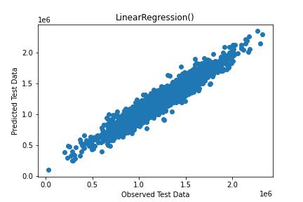
predictions = lm.predict(X_test)

and plot the result

plt.scatter(Y_test,predictions)
plt.title(‘LinearRegression()’)
plt.xlabel(‘Observed Test Data’)
plt.ylabel(‘Predicted Test Data’)
plt.savefig(‘testlinreg.jpg’)

Let’s compare it with the xgboost algorithm

import xgboost as xg
reg = xg.XGBRegressor(objective =’reg:linear’,
n_estimators = 1000, seed = 123)

reg.fit(X_train,Y_train)
predictions = reg.predict(X_test)

We can see that LinearRegression() yields the more accurate prediction than XGBRegressor(). The same considerations apply to the sklearn algorithms (SVR, TweedieRegressor, RandomForestRegressor, etc.).

Case 2: CA

Let’s look at the median house prices for California districts derived from the 1990 census. This is the dataset used in the second chapter of Aurélien Géron’s recent book ‘Hands-On Machine learning with Scikit-Learn and TensorFlow’. The ultimate goal of end-to-end ML is to build a RE prediction engine capable of minimizing error rate RMSE (Root Mean Square Error) or MAE (Mean Absolute Error) or any other metrics of interest.

Let’s set the working directory YOURPATH

import os

os.chdir(‘YOURPATH’)
os. getcwd()

and import libraries

import pandas as pd
import matplotlib.pyplot as plt
import numpy as np

Let’s read the data

housing_data = pd.read_csv(“housing.csv”)
housing_data

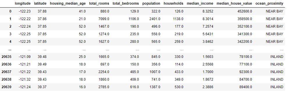
representing 20640 rows × 10 columns.

The data info is

housing_data.info()

<class 'pandas.core.frame.DataFrame'>
RangeIndex: 20640 entries, 0 to 20639
Data columns (total 10 columns):
 #   Column              Non-Null Count  Dtype  
---  ------              --------------  -----  
 0   longitude           20640 non-null  float64
 1   latitude            20640 non-null  float64
 2   housing_median_age  20640 non-null  float64
 3   total_rooms         20640 non-null  float64
 4   total_bedrooms      20433 non-null  float64
 5   population          20640 non-null  float64
 6   households          20640 non-null  float64
 7   median_income       20640 non-null  float64
 8   median_house_value  20640 non-null  float64
 9   ocean_proximity     20640 non-null  object 
dtypes: float64(9), object(1)
memory usage: 1.6+ MB

Let’s plot the ocean proximity bar chart

housing_data[“ocean_proximity”].value_counts().plot(kind=”barh”)

We can see that “ISLAND” value_counts is negligible compared to “1H OCEAN”.

The descriptive statistics of input data is

housing_data.describe()

Let’s plot the histogram of median income

housing_data[“median_income”].hist()

Let’s introduce 5 categories of median income

housing_data[“income_cat”]= pd.cut(housing_data[“median_income”],
bins=[0,1.5,3.0,4.5,6, np.inf],
labels=[1,2,3,4,5])
housing_data[“income_cat”].value_counts()

3    7236
2    6581
4    3639
5    2362
1     822
Name: income_cat, dtype: int64

and plot histograms of these categories

housing_data[“income_cat”].hist()

Let’s introduce the target variable median_house_value and the model features

y = housing_data[“median_house_value”]
X= housing_data.drop(“median_house_value”,axis=1)
X

with 20640 rows × 10 columns.

Let’s split the data into 33% and 66% for Training and Testing, respectively

from sklearn.model_selection import train_test_split

X_train, X_test, y_train, y_test = train_test_split(X, y, test_size=0.33)

Let’s select StratifiedShuffleSplit that provides train/test indices to split data in train/test sets. This cross-validation object is a merge of StratifiedKFold and ShuffleSplit, which returns stratified randomized folds. The folds are made by preserving the percentage of samples for each class

from sklearn.model_selection import StratifiedShuffleSplit
split = StratifiedShuffleSplit(n_splits=1, test_size=0.2,random_state=42)
for train_index, test_index in split.split(housing_data,housing_data[“income_cat”]):
strat_train_set = housing_data.loc[train_index]
strat_test_set = housing_data.loc[test_index]

Let’s check strat_test_set value count in terms of income_cat as a fraction

strat_test_set[“income_cat”].value_counts() / len(strat_test_set)

3    0.350533
2    0.318798
4    0.176357
5    0.114341
1    0.039971
Name: income_cat, dtype: float64

We can see only 4% of strat_test_set belongs to income_cat=1 as compared to 35% of strat_test_set that belongs to income_cat=3.

Let’s plot the histograms of training data

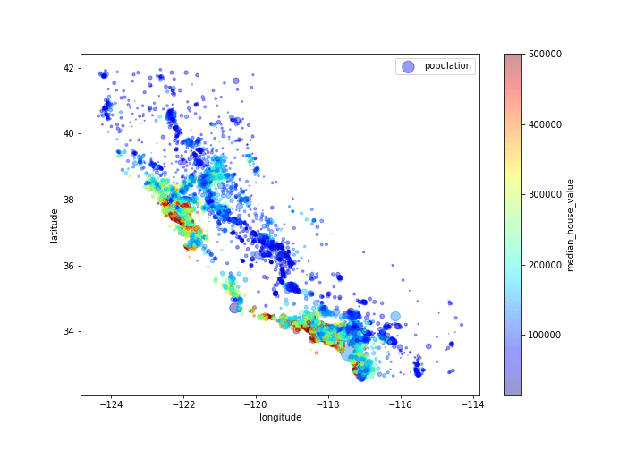
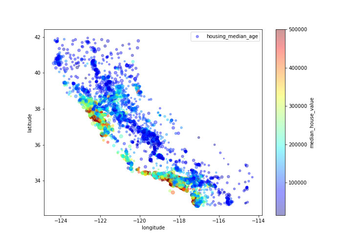
Let’s plot the geo-location map population and housing median age vs median house value

housing.plot(kind=”scatter”,x=”longitude”,y=”latitude”,alpha=0.4,
s = housing[“population”]/100, label=”population”,figsize=(10,7),
c=”median_house_value”,cmap=plt.get_cmap(“jet”),colorbar=True,
sharex=False)
plt.savefig(‘camappopulationhouseprice.png’)

housing.plot(kind=”scatter”,x=”longitude”,y=”latitude”,alpha=0.4,
s = housing[“housing_median_age”], label=”housing_median_age”,figsize=(10,7),
c=”median_house_value”,cmap=plt.get_cmap(“jet”),colorbar=True,
sharex=False)
plt.savefig(‘camaphouseagehouseprice.png’)

Let’s look at the housing correlation matrix

housing.corr()

and plot the corresponding annotated heatmap

import seaborn as sns
corr = housing.corr()
mask = np.triu(np.ones_like(corr,dtype=bool))

f, ax = plt.subplots(figsize= (11, 9))
cmap = sns.diverging_palette(230, 20, as_cmap = True)
sns_plot=sns.heatmap(corr,mask=mask,cmap=cmap, vmax=.3,center=0,annot = True,
square=True, linewidths=0.5, cbar_kws={“shrink”:.5})
fig = sns_plot.get_figure()
fig.savefig(“cacorrheatmap.png”)

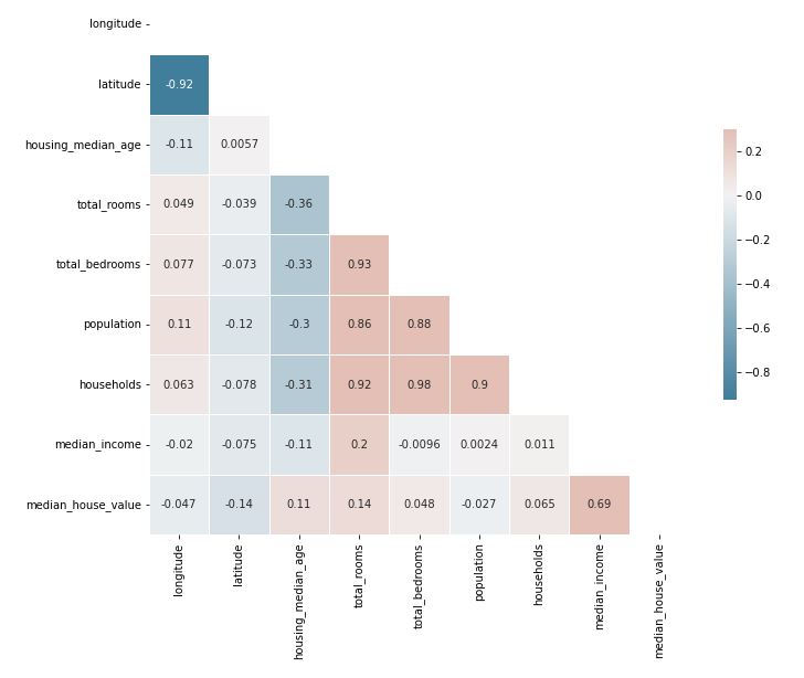
We can see that median_income is the most dominant factor that affects median_house_price.

Let’s check rows for missing values

sample_incomplete_rows= housing[housing.isnull().any(axis=1)].head()
sample_incomplete_rows

while dropping the column with no values

sample_incomplete_rows.dropna(subset=[“total_bedrooms”])

longitude latitude housing_median_age total_rooms total_bedrooms population households median_income median_house_value ocean_proximity

Let’s fill NaN with median values

median = housing[‘total_bedrooms’].median()
sample_incomplete_rows[‘total_bedrooms’].fillna(median,inplace=True)
sample_incomplete_rows

Let’s apply the SimpleImputer method with strategy =’median’

from sklearn.impute import SimpleImputer
imputer = SimpleImputer(strategy =’median’)
housing_num = housing.select_dtypes(include=(np.number))
housing_num

from sklearn import impute
imputer.fit(housing_num)
SimpleImputer(strategy=’median’)

SimpleImputer(strategy='median')

X = imputer.transform(housing_num)
housing_tr = pd.DataFrame(X, columns = housing_num.columns,index=housing_num.index)
housing_tr

Recall that

imputer.strategy

'median'

Let’s encode categorical variables to convert non-numerical data into numerical data to create inferences

housing_cat =housing[[‘ocean_proximity’]]
housing_cat.head(10)

Let’s apply OrdinalEncoder to this variable

from sklearn.preprocessing import OrdinalEncoder

ordinal_encoder= OrdinalEncoder()
housing_cat_encoded=ordinal_encoder.fit_transform(housing_cat)
housing_cat_encoded[:10]

array([[1.],
       [4.],
       [1.],
       [4.],
       [0.],
       [3.],
       [0.],
       [0.],
       [0.],
       [0.]])

Let’s apply OneHotEncoder to housing_cat

from sklearn.preprocessing import OneHotEncoder
cat_encoder = OneHotEncoder(sparse=False)
housing_cat_1hot = cat_encoder.fit_transform(housing_cat)
housing_cat_1hot

array([[0., 1., 0., 0., 0.],
       [0., 0., 0., 0., 1.],
       [0., 1., 0., 0., 0.],
       ...,
       [1., 0., 0., 0., 0.],
       [1., 0., 0., 0., 0.],
       [0., 1., 0., 0., 0.]])

Let’s define the feature_engineering function

def feature_engineering(data):
data[‘bedrooms_per_household’] = data[‘total_bedrooms’]/data[‘households’]
data[‘population_per_households’]=data[‘population’]/data[‘households’]
data[‘rooms_per_households’]=data[‘total_rooms’]/data[‘households’]

return data

and apply this function to the housing data

housing_feature_engineered = feature_engineering(housing_num)
housing_feature_engineered

Let’s scale our data

from sklearn.preprocessing import StandardScaler

scaler = StandardScaler()

housing_scaled = scaler.fit_transform(housing_feature_engineered)
housing_scaled

array([[-0.94135046,  1.34743822,  0.02756357, ...,  0.05896205,
         0.00622264,  0.01739526],
       [ 1.17178212, -1.19243966, -1.72201763, ...,  0.02830837,
        -0.04081077,  0.56925554],
       [ 0.26758118, -0.1259716 ,  1.22045984, ..., -0.1286475 ,
        -0.07537122, -0.01802432],
       ...,
       [-1.5707942 ,  1.31001828,  1.53856552, ..., -0.26257303,
        -0.03743619, -0.5092404 ],
       [-1.56080303,  1.2492109 , -1.1653327 , ...,  0.11548226,
        -0.05915604,  0.32814891],
       [-1.28105026,  2.02567448, -0.13148926, ...,  0.05505203,
         0.00657083,  0.01407228]])

Let’s create the ML input data

ml_input_data = np.hstack([housing_cat_1hot, housing_scaled])
ml_input_data

array([[ 0.        ,  1.        ,  0.        , ...,  0.05896205,
         0.00622264,  0.01739526],
       [ 0.        ,  0.        ,  0.        , ...,  0.02830837,
        -0.04081077,  0.56925554],
       [ 0.        ,  1.        ,  0.        , ..., -0.1286475 ,
        -0.07537122, -0.01802432],
       ...,
       [ 1.        ,  0.        ,  0.        , ..., -0.26257303,
        -0.03743619, -0.5092404 ],
       [ 1.        ,  0.        ,  0.        , ...,  0.11548226,
        -0.05915604,  0.32814891],
       [ 0.        ,  1.        ,  0.        , ...,  0.05505203,
         0.00657083,  0.01407228]])

Let’s define the entire ETL pipeline to be applied to the housing data

housing = strat_train_set.drop(“median_house_value”, axis=1)
housing_labels = strat_train_set[“median_house_value”].copy()

def data_transformations(data):

### Separate Labels if they Exist ###

if "median_house_value" in data.columns:
    labels = data["median_house_value"]
    data = data.drop("median_house_value", axis=1)

else:
    labels = None

### Feature Engineering ###
feature_engineered_data = feature_engineering(data)
features = list(feature_engineered_data.columns) # Creating a list of our features for future use

### Imputing Data ###
from sklearn.impute import SimpleImputer
imputer = SimpleImputer(strategy="median")

housing_num = feature_engineered_data.select_dtypes(include=[np.number])
imputed = imputer.fit_transform(housing_num)

### Encoding Categorical Data ###
housing_cat = feature_engineered_data.select_dtypes(exclude=[np.number])

from sklearn.preprocessing import OneHotEncoder
cat_encoder = OneHotEncoder(sparse=False)
housing_cat_1hot = cat_encoder.fit_transform(housing_cat)
features = features + cat_encoder.categories_[0].tolist()
features.remove("ocean_proximity") # We're encoding this variable, so we don't need it in our list anymore


### Scaling Numerical Data ###
from sklearn.preprocessing import StandardScaler
scaler = StandardScaler()

housing_scaled = scaler.fit_transform(imputed)

### Concatening all Data ###
output = np.hstack([housing_scaled, housing_cat_1hot])

return output, labels, features

cat_encoder.categories_[0].tolist()

['<1H OCEAN', 'INLAND', 'ISLAND', 'NEAR BAY', 'NEAR OCEAN']

Let’s select and train the model
train_data, train_labels, features = data_transformations(strat_train_set)
train_data

array([[-0.94135046,  1.34743822,  0.02756357, ...,  0.        ,
         0.        ,  0.        ],
       [ 1.17178212, -1.19243966, -1.72201763, ...,  0.        ,
         0.        ,  1.        ],
       [ 0.26758118, -0.1259716 ,  1.22045984, ...,  0.        ,
         0.        ,  0.        ],
       ...,
       [-1.5707942 ,  1.31001828,  1.53856552, ...,  0.        ,
         0.        ,  0.        ],
       [-1.56080303,  1.2492109 , -1.1653327 , ...,  0.        ,
         0.        ,  0.        ],
       [-1.28105026,  2.02567448, -0.13148926, ...,  0.        ,
         0.        ,  0.        ]])

Let’s test the model

test_data, test_labels, features = data_transformations(strat_test_set)
test_data

array([[ 0.57507019, -0.69657252,  0.0329564 , ...,  0.        ,
         0.        ,  0.        ],
       [-0.43480141, -0.33466769, -0.36298077, ...,  0.        ,
         0.        ,  0.        ],
       [ 0.54522177, -0.63547171,  0.58726843, ...,  0.        ,
         0.        ,  0.        ],
       ...,
       [-0.08656982, -0.54617051,  1.14158047, ...,  0.        ,
         0.        ,  0.        ],
       [ 0.81385757, -0.92687559,  0.11214383, ...,  0.        ,
         0.        ,  0.        ],
       [ 0.49049967, -0.66367208,  0.58726843, ...,  0.        ,
         0.        ,  0.        ]])

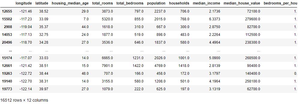
We have got the train labels

train_labels

12655     72100.0
15502    279600.0
2908      82700.0
14053    112500.0
20496    238300.0
           ...   
15174    268500.0
12661     90400.0
19263    140400.0
19140    258100.0
19773     62700.0
Name: median_house_value, Length: 16512, dtype: float64

and the features

features

['longitude',
 'latitude',
 'housing_median_age',
 'total_rooms',
 'total_bedrooms',
 'population',
 'households',
 'median_income',
 'bedrooms_per_household',
 'population_per_households',
 'rooms_per_households',
 '<1H OCEAN',
 'INLAND',
 'ISLAND',
 'NEAR BAY',
 'NEAR OCEAN']

Following Case 1 (see above), let’s apply the Linear Regression

from sklearn.linear_model import LinearRegression
lin_reg = LinearRegression()
lin_reg.fit(train_data,train_labels)

LinearRegression()

Let’s compare original and predicted values

original_values = test_labels[:5]
predicted_values = lin_reg.predict(test_data[:5])
comparison_dataframe = pd.DataFrame(data={“Original Values”:original_values, “Predicted Values”:predicted_values})

comparison_dataframe[“Differences”] = comparison_dataframe[“Original Values”] – comparison_dataframe[“Predicted Values”]

comparison_dataframe

Let’s check the MSE metric

from sklearn.metrics import mean_squared_error

lin_mse = mean_squared_error(original_values,predicted_values)
lin_rmse = np.sqrt(lin_mse)
lin_rmse

78489.87096668077

Let’s check the MAE metric

from sklearn.metrics import mean_absolute_error

lin_mae = mean_absolute_error(original_values, predicted_values)
lin_mae

71328.53325778323

Let’s apply the Decision Tree algorithm

from sklearn.tree import DecisionTreeRegressor
tree_reg = DecisionTreeRegressor(random_state=42)
tree_reg.fit(train_data,train_labels)

DecisionTreeRegressor(random_state=42)

train_predictions = tree_reg.predict(train_data)
tree_mse = mean_squared_error(train_labels, train_predictions)
tree_rmse = np.sqrt(tree_mse)
tree_rmse

0.0

Let’s compute the cross-validation score

from sklearn.model_selection import cross_val_score

scores = cross_val_score(tree_reg, train_data, train_labels, scoring=”neg_mean_squared_error”, cv=10)
tree_rmse_scores = np.sqrt(-scores)

def display_scores(scores):
print(“Scores:”, scores)
print(“Mean:”, scores.mean())
print(“Standard deviation:”, scores.std())

display_scores(tree_rmse_scores)

Scores: [70819.83674558 70585.09139446 69861.50467212 73083.46385442
 66246.62162221 74093.76616605 77298.21284135 70265.05374821
 70413.46481703 72693.02785945]
Mean: 71536.00437208822
Standard deviation: 2802.723447985299

Let’s apply the Random Forest Regressor

rom sklearn.ensemble import RandomForestRegressor

forest_reg = RandomForestRegressor(n_estimators=100, random_state=42)
forest_reg.fit(train_data, train_labels)

RandomForestRegressor(random_state=42)

train_predictions = forest_reg.predict(train_data)
forest_mse = mean_squared_error(train_labels, train_predictions)
forest_rmse = np.sqrt(forest_mse)
forest_rmse

18797.81343373367

Let’s select the corresponding cross_val_score

from sklearn.model_selection import cross_val_score

forest_scores = cross_val_score(forest_reg, train_data, train_labels,
scoring=”neg_mean_squared_error”, cv=10)
forest_rmse_scores = np.sqrt(-forest_scores)
display_scores(forest_rmse_scores)

Scores: [51667.47890087 49581.77674843 46845.77133522 52127.48739086
 48082.89639917 51050.84681689 53027.94987383 50218.59780997
 48609.03966622 54669.97457167]
Mean: 50588.18195131385
Standard deviation: 2273.9929947683154

Let’s try 12 (3×4) combinations of hyperparameters and then try then try 6 (2×3) combinations with bootstrap set as False using GridSearchCV

from sklearn.model_selection import GridSearchCV

param_grid = [
# try 12 (3×4) combinations of hyperparameters
{‘n_estimators’: [3, 10, 30], ‘max_features’: [2, 4, 6, 8]},
# then try 6 (2×3) combinations with bootstrap set as False
{‘bootstrap’: [False], ‘n_estimators’: [3, 10], ‘max_features’: [2, 3, 4]},
]

forest_reg = RandomForestRegressor(random_state=42)

Let’s train across 5 folds, that’s a total of (12+6)*5=90 rounds of training

grid_search = GridSearchCV(forest_reg, param_grid, cv=5,
scoring=’neg_mean_squared_error’,
return_train_score=True)
grid_search.fit(train_data, train_labels)

GridSearchCV(cv=5, estimator=RandomForestRegressor(random_state=42),
             param_grid=[{'max_features': [2, 4, 6, 8],
                          'n_estimators': [3, 10, 30]},
                         {'bootstrap': [False], 'max_features': [2, 3, 4],
                          'n_estimators': [3, 10]}],
             return_train_score=True, scoring='neg_mean_squared_error')

Let’s see the best estimator

grid_search.best_estimator_

RandomForestRegressor(max_features=6, n_estimators=30, random_state=42)

The results of grid search cv are as follows

cvres = grid_search.cv_results_
for mean_score, params in zip(cvres[“mean_test_score”], cvres[“params”]):
print(np.sqrt(-mean_score), params)

64441.33583774864 {'max_features': 2, 'n_estimators': 3}
55010.78729315784 {'max_features': 2, 'n_estimators': 10}
52756.90743676946 {'max_features': 2, 'n_estimators': 30}
60419.95105027927 {'max_features': 4, 'n_estimators': 3}
52548.760723492225 {'max_features': 4, 'n_estimators': 10}
50475.03023921768 {'max_features': 4, 'n_estimators': 30}
58658.87553276854 {'max_features': 6, 'n_estimators': 3}
51688.259845013825 {'max_features': 6, 'n_estimators': 10}
49602.83903888296 {'max_features': 6, 'n_estimators': 30}
57764.545176887186 {'max_features': 8, 'n_estimators': 3}
51906.606161086886 {'max_features': 8, 'n_estimators': 10}
49851.77165193962 {'max_features': 8, 'n_estimators': 30}
63137.43571927858 {'bootstrap': False, 'max_features': 2, 'n_estimators': 3}
54419.40582754731 {'bootstrap': False, 'max_features': 2, 'n_estimators': 10}
58195.29390064867 {'bootstrap': False, 'max_features': 3, 'n_estimators': 3}
52168.74519952844 {'bootstrap': False, 'max_features': 3, 'n_estimators': 10}
59520.17602710436 {'bootstrap': False, 'max_features': 4, 'n_estimators': 3}
51828.25647287002 {'bootstrap': False, 'max_features': 4, 'n_estimators': 10}

The corresponding dataframe is

pd.DataFrame(grid_search.cv_results_)

representing 18 rows × 23 columns.

Let’s compare it to RandomizedSearchCV

from sklearn.model_selection import RandomizedSearchCV
from scipy.stats import randint

param_distribs = {
‘n_estimators’: randint(low=1, high=200),
‘max_features’: randint(low=1, high=8),
}

forest_reg = RandomForestRegressor(random_state=42)
rnd_search = RandomizedSearchCV(forest_reg, param_distributions=param_distribs,
n_iter=10, cv=5, scoring=’neg_mean_squared_error’, random_state=42)
rnd_search.fit(train_data, train_labels)

RandomizedSearchCV(cv=5, estimator=RandomForestRegressor(random_state=42),
                   param_distributions={'max_features': <scipy.stats._distn_infrastructure.rv_frozen object at 0x000001669BCE8220>,
                                        'n_estimators': <scipy.stats._distn_infrastructure.rv_frozen object at 0x000001669BCE0640>},
                   random_state=42, scoring='neg_mean_squared_error')

The results are as follows

cvres = rnd_search.cv_results_
for mean_score, params in zip(cvres[“mean_test_score”], cvres[“params”]):
print(np.sqrt(-mean_score), params)

48881.00597871309 {'max_features': 7, 'n_estimators': 180}
51634.61963021687 {'max_features': 5, 'n_estimators': 15}
50312.55245794906 {'max_features': 3, 'n_estimators': 72}
50952.54821857023 {'max_features': 5, 'n_estimators': 21}
49063.34454115586 {'max_features': 7, 'n_estimators': 122}
50317.63324666772 {'max_features': 3, 'n_estimators': 75}
50173.504527094505 {'max_features': 3, 'n_estimators': 88}
49248.29804214526 {'max_features': 5, 'n_estimators': 100}
50054.94886918995 {'max_features': 3, 'n_estimators': 150}
64847.94779269648 {'max_features': 5, 'n_estimators': 2}

Let’s look at the feature importances

feature_importances = grid_search.best_estimator_.feature_importances_
feature_importances

array([8.46978272e-02, 7.69983975e-02, 4.08715796e-02, 1.67325719e-02,
       1.71418340e-02, 1.73518185e-02, 1.56303531e-02, 3.39824215e-01,
       2.30528104e-02, 1.04033701e-01, 8.64983594e-02, 1.29273143e-02,
       1.54663950e-01, 7.22217547e-05, 3.62205279e-03, 5.88099358e-03])

The corresponding list is as follows

feature_importance_list = list(zip(features, feature_importances.tolist()))
feature_importance_list

[('longitude', 0.0846978271965227),
 ('latitude', 0.07699839747855737),
 ('housing_median_age', 0.040871579612884096),
 ('total_rooms', 0.016732571900462085),
 ('total_bedrooms', 0.01714183399184058),
 ('population', 0.0173518184721046),
 ('households', 0.015630353131298083),
 ('median_income', 0.3398242154869636),
 ('bedrooms_per_household', 0.023052810363875926),
 ('population_per_households', 0.10403370064780083),
 ('rooms_per_households', 0.08649835942626646),
 ('<1H OCEAN', 0.012927314349565632),
 ('INLAND', 0.15466394981681342),
 ('ISLAND', 7.222175467748088e-05),
 ('NEAR BAY', 0.003622052794433035),
 ('NEAR OCEAN', 0.005880993575933963)]

We can plot this list as the vertical bar container that consists of 16 columns

plt.barh(y=features, width=feature_importances.tolist())

The final model RMSE is given by

final_model = grid_search.best_estimator_

final_predictions = final_model.predict(test_data)

final_mse = mean_squared_error(test_labels, final_predictions)
final_rmse = np.sqrt(final_mse)

final_rmse

63301.179203602675

This can be modified further using various feature selection methods.

Thus, median_income is the most important feature. The best result is achieved using RandomForestRegressor + RandomizedSearchCV. The trained prediction of

RandomForestRegressor(random_state=42) 
yields rmse=18797.8+/-2274,

whreas min (mean_test_score) yields

48881

with ‘max_features’: 7, ‘n_estimators’: 180.

Case 3: IA

For this case study, the primary objective was to create and assess advanced ML/AI models to accurately predict house prices based on the Ames dataset. It was compiled by Dean De Cock for use in data science education. It’s an incredible alternative for data scientists looking for a modernized and expanded version of the often cited Boston Housing dataset. 

The data set includes around 3000 records of house sales in Ames, Iowa between 2006 – 2010 and contains 79 explanatory variables detailing various aspects of residential homes such as square footage, number of rooms and sale year. The data is split into a training set, which will be used to create the model and a test set, which will be used to test model performance.

Results can provide insights on the pricing of real estate assets just by plugging in the house characteristics and letting the model return a price. In addition, the ML/AI output can provide information on which features of a new house are more valuable for potential house buyers. Source code: GitHub.

The general ETL Python workflow to create the model is as follows:

1. Data preprocessing
2. Exploratory data analysis/Feature Engineering
3. Model training & hyperparameter tuning
4. Model diagnostics & evaluation
5. Result interpretation

Let’s set the working directory YOURPATH

import os
os.chdir(‘YOURPATH’)
os. getcwd()

Let’s import libraries and download train/test Ames datasets
%matplotlib inline
import numpy as np
import pandas as pd
import matplotlib.pyplot as plt
import scipy.stats as stats
import sklearn.linear_model as linear_model
import seaborn as sns
import xgboost as xgb
from sklearn.model_selection import KFold
from IPython.display import HTML, display
from sklearn.manifold import TSNE
from sklearn.cluster import KMeans
from sklearn.decomposition import PCA
from sklearn.preprocessing import StandardScaler

pd.options.display.max_rows = 1000
pd.options.display.max_columns = 20

train = pd.read_csv(‘train.csv’)
test = pd.read_csv(‘test.csv’)

Let’s get the dimensions of the train and test data
print(“Training data set dimension : {}”.format(train.shape))
print(“Testing data set dimension : {}”.format(test.shape))

Training data set dimension : (2051, 81)
Testing data set dimension : (879, 80)

Let’s look at the continuous features
numerical_cols = [col for col in train.columns if train.dtypes[col] != ‘object’]
numerical_cols.remove(‘SalePrice’)
numerical_cols.remove(‘Id’)
print(““122)
print(“Continuous features”)
print(““122)
print(numerical_cols)
print(““122)
print(“count of continuous features:”,len(numerical_cols))
print(““122)

Continuous features
***************************************************************************
['PID', 'MS SubClass', 'Lot Frontage', 'Lot Area', 'Overall Qual', 'Overall Cond', 'Year Built', 'Year Remod/Add', 'Mas Vnr Area', 'BsmtFin SF 1', 'BsmtFin SF 2', 'Bsmt Unf SF', 'Total Bsmt SF', '1st Flr SF', '2nd Flr SF', 'Low Qual Fin SF', 'Gr Liv Area', 'Bsmt Full Bath', 'Bsmt Half Bath', 'Full Bath', 'Half Bath', 'Bedroom AbvGr', 'Kitchen AbvGr', 'TotRms AbvGrd', 'Fireplaces', 'Garage Yr Blt', 'Garage Cars', 'Garage Area', 'Wood Deck SF', 'Open Porch SF', 'Enclosed Porch', '3Ssn Porch', 'Screen Porch', 'Pool Area', 'Misc Val', 'Mo Sold', 'Yr Sold']
***************************************************************************
count of continuous features: 37

Let’s look at the categorical features
categorical_cols = [col for col in train.columns if train.dtypes[col] == ‘object’]
print(““122)
print(“categorical features”)
print(““122)
print(categorical_cols)
print(““122)
print(“count of categorical features:”,len(categorical_cols))
print(““122)

categorical features
***************************************************************************
['MS Zoning', 'Street', 'Alley', 'Lot Shape', 'Land Contour', 'Utilities', 'Lot Config', 'Land Slope', 'Neighborhood', 'Condition 1', 'Condition 2', 'Bldg Type', 'House Style', 'Roof Style', 'Roof Matl', 'Exterior 1st', 'Exterior 2nd', 'Mas Vnr Type', 'Exter Qual', 'Exter Cond', 'Foundation', 'Bsmt Qual', 'Bsmt Cond', 'Bsmt Exposure', 'BsmtFin Type 1', 'BsmtFin Type 2', 'Heating', 'Heating QC', 'Central Air', 'Electrical', 'Kitchen Qual', 'Functional', 'Fireplace Qu', 'Garage Type', 'Garage Finish', 'Garage Qual', 'Garage Cond', 'Paved Drive', 'Pool QC', 'Fence', 'Misc Feature', 'Sale Type']
***************************************************************************
count of categorical features: 42

and check unique column values below

print(‘unique column values’)
train.apply(lambda x: len(x.unique())).sort_values(ascending=False).head(10)

unique column values

Out[6]:

Id               2051
PID              2051
Lot Area         1476
Gr Liv Area      1053
Bsmt Unf SF       968
1st Flr SF        915
Total Bsmt SF     893
SalePrice         828
BsmtFin SF 1      822
Garage Area       515
dtype: int64

Let’s check the sorted cardinality train values

cardinality = train[categorical_cols].apply(lambda x: len(x.unique()))
cardinality.sort_values(ascending=False).head(30)

Neighborhood      28
Exterior 2nd      15
Exterior 1st      15
Sale Type          9
Condition 1        9
House Style        8
Functional         8
Condition 2        8
Garage Type        7
BsmtFin Type 2     7
BsmtFin Type 1     7
MS Zoning          7
Bsmt Qual          6
Roof Matl          6
Misc Feature       6
Garage Cond        6
Garage Qual        6
Foundation         6
Fireplace Qu       6
Bsmt Cond          6
Roof Style         6
Heating            5
Fence              5
Pool QC            5
Electrical         5
Bldg Type          5
Bsmt Exposure      5
Exter Cond         5
Mas Vnr Type       5
Lot Config         5
dtype: int64

and the cardinality test values

cardinality = test[categorical_cols].apply(lambda x: len(x.unique()))
cardinality.sort_values(ascending=False).head(40)

Neighborhood      26
Exterior 2nd      16
Exterior 1st      13
Sale Type         10
Condition 1        9
House Style        8
Garage Type        7
BsmtFin Type 2     7
BsmtFin Type 1     7
Garage Cond        6
Fireplace Qu       6
Functional         6
Foundation         6
Mas Vnr Type       6
MS Zoning          6
Roof Matl          6
Roof Style         6
Bsmt Qual          6
Kitchen Qual       5
Exter Cond         5
Fence              5
Garage Qual        5
Bsmt Exposure      5
Lot Config         5
Bldg Type          5
Electrical         5
Misc Feature       4
Garage Finish      4
Lot Shape          4
Land Contour       4
Exter Qual         4
Heating QC         4
Heating            4
Bsmt Cond          4
Condition 2        4
Land Slope         3
Alley              3
Paved Drive        3
Pool QC            3
Utilities          2
dtype: int64

Let’s check good and bad train+test column lists

good_label_cols = [col for col in categorical_cols if set(test[col]).issubset(set(train[col]))]
len(good_label_cols)

34

bad_label_cols = list(set(categorical_cols)-set(good_label_cols))
bad_label_cols

['Sale Type',
 'Exterior 1st',
 'Heating',
 'Roof Matl',
 'Electrical',
 'Exterior 2nd',
 'Mas Vnr Type',
 'Kitchen Qual']

Let’s plot the count of missing values in the training data column features

cols_with_missing = train.isnull().sum()
cols_with_missing = cols_with_missing[cols_with_missing>0]
cols_with_missing.sort_values(inplace=True)
fig, ax = plt.subplots(figsize=(7,6))
width = 0.70 # the width of the bars
ind = np.arange(len(cols_with_missing)) # the x locations for the groups
ax.barh(ind, cols_with_missing, width, color=”blue”)
ax.set_yticks(ind+width/2)
ax.set_yticklabels(cols_with_missing.index, minor=False)
plt.xlabel(‘Count’)
plt.ylabel(‘Features’)
plt.savefig(“amesfeaturesmissingvalues.png”)

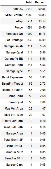
Let’s count the percentage of missing values in training data
print(‘Percentage of missing values in each columns’)

total = train.isnull().sum().sort_values(ascending=False)
percent = (train.isnull().sum()/train.isnull().count()).sort_values(ascending=False)
missing_data_tr = pd.concat([total, round(percent*100,2)], axis=1, keys=[‘Total’, ‘Percent’])
missing_data_tr[missing_data_tr.Total>=1]

Percentage of missing values in each columns

Similarly, we plot the count of missing values in the test data column features

cols_with_missing = test.isnull().sum()
cols_with_missing = cols_with_missing[cols_with_missing>0]
cols_with_missing.sort_values(inplace=True)
fig, ax = plt.subplots(figsize=(7,6))
width = 0.70 # the width of the bars
ind = np.arange(len(cols_with_missing)) # the x locations for the groups
ax.barh(ind, cols_with_missing, width, color=”blue”)
ax.set_yticks(ind+width/2)
ax.set_yticklabels(cols_with_missing.index, minor=False)
plt.xlabel(‘Count’)
plt.ylabel(‘Features’)

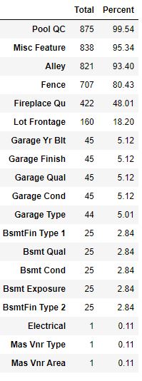
and the percentage of missing values in test data columns

print(‘Percentage of missing values in each columns’)

total = test.isnull().sum().sort_values(ascending=False)
percent = (test.isnull().sum()/test.isnull().count()).sort_values(ascending=False)
missing_data_te = pd.concat([total, round(percent*100,2)], axis=1, keys=[‘Total’, ‘Percent’])
missing_data_te[missing_data_te.Total>=1]

Percentage of missing values in each columns

Let’s prepare the data for ML.

Separate features and target variable SalePrice
X_train = train_data.drop([‘SalePrice’], axis=1)
y = train_data.SalePrice

and concatenate train and test data
X = pd.concat([X_train, test_data], axis=0)

let’s apply SimpleImputer to deal with missing values

from sklearn.impute import SimpleImputer

group_1 = [
‘PoolQC’, ‘MiscFeature’, ‘Alley’, ‘Fence’, ‘FireplaceQu’, ‘GarageType’,
‘GarageFinish’, ‘GarageQual’, ‘GarageCond’, ‘BsmtQual’, ‘BsmtCond’,
‘BsmtExposure’, ‘BsmtFinType1’, ‘BsmtFinType2’, ‘MasVnrType’
]
X[group_1] = X[group_1].fillna(“None”)

group_2 = [
‘GarageArea’, ‘GarageCars’, ‘BsmtFinSF1’, ‘BsmtFinSF2’, ‘BsmtUnfSF’,
‘TotalBsmtSF’, ‘BsmtFullBath’, ‘BsmtHalfBath’, ‘MasVnrArea’
]

X[group_2] = X[group_2].fillna(0)

group_3a = [
‘Functional’, ‘MSZoning’, ‘Electrical’, ‘KitchenQual’, ‘Exterior1st’,
‘Exterior2nd’, ‘SaleType’, ‘Utilities’
]

imputer = SimpleImputer(strategy=’most_frequent’)
X[group_3a] = pd.DataFrame(imputer.fit_transform(X[group_3a]), index=X.index)

X.LotFrontage = X.LotFrontage.fillna(X.LotFrontage.mean())
X.GarageYrBlt = X.GarageYrBlt.fillna(X.YearBuilt)

Let’s check that there are no remaining missing values

sum(X.isnull().sum())

0

Let’s drop outliers in GrLivArea and SalePrice (based on Ames EDA)

outlier_index = train_data[(train_data.GrLivArea > 4000)
& (train_data.SalePrice < 200000)].index
X.drop(outlier_index, axis=0, inplace=True)
y.drop(outlier_index, axis=0, inplace=True)

Let’s apply label encoding to the categorical columns

from sklearn.preprocessing import LabelEncoder

label_encoding_cols = [
“Alley”, “BsmtCond”, “BsmtExposure”, “BsmtFinType1”, “BsmtFinType2”,
“BsmtQual”, “ExterCond”, “ExterQual”, “FireplaceQu”, “Functional”,
“GarageCond”, “GarageQual”, “HeatingQC”, “KitchenQual”, “LandSlope”,
“LotShape”, “PavedDrive”, “PoolQC”, “Street”, “Utilities”
]

label_encoder = LabelEncoder()

for col in label_encoding_cols:
X[col] = label_encoder.fit_transform(X[col])

Let’ transform numerical variables to categorical variables
to_factor_cols = [‘YrSold’, ‘MoSold’, ‘MSSubClass’]

for col in to_factor_cols:
X[col] = X[col].apply(str)

Let’s apply feature scaling using RobustScaler
from sklearn.preprocessing import RobustScaler
numerical_cols = list(X.select_dtypes(exclude=[‘object’]).columns)
scaler = RobustScaler()
X[numerical_cols] = scaler.fit_transform(X[numerical_cols])

followed by one-hot encoding
X = pd.get_dummies(X, drop_first=True)
print(“X.shape:”, X.shape)

X.shape: (2917, 237)

Let’s define the train and test columns

ntest = len(test_data)
X_train = X.iloc[:-ntest, :]
X_test = X.iloc[-ntest:, :]
print(“X_train.shape:”, X_train.shape)
print(“X_test.shape:”, X_test.shape)

X_train.shape: (1458, 237)
X_test.shape: (1459, 237)

let’s perform modeling
from sklearn.model_selection import KFold, cross_val_score

n_folds = 5

def getRMSLE(model):
“””
Return the average RMSLE over all folds of training data.
“””
# Set KFold to shuffle data before the split
kf = KFold(n_folds, shuffle=True, random_state=42)

# Get RMSLE score
rmse = np.sqrt(-cross_val_score(
    model, X_train, y, scoring="neg_mean_squared_error", cv=kf))

return rmse.mean()

Let’s apply regularized regressions
from sklearn.linear_model import Ridge, Lasso

lambda_list = list(np.linspace(20, 25, 101))

rmsle_ridge = [getRMSLE(Ridge(alpha=lambda_)) for lambda_ in lambda_list]
rmsle_ridge = pd.Series(rmsle_ridge, index=lambda_list)

rmsle_ridge.plot(title=”RMSLE by lambda”)
plt.xlabel(“Lambda”)
plt.ylabel(“RMSLE”)
plt.savefig(“amesridgelambdarmsle.png”)
print(“Best lambda:”, rmsle_ridge.idxmin())
print(“RMSLE:”, rmsle_ridge.min())

Ridge lambda:

Best lambda: 22.9
RMSLE: 0.11409306668450883

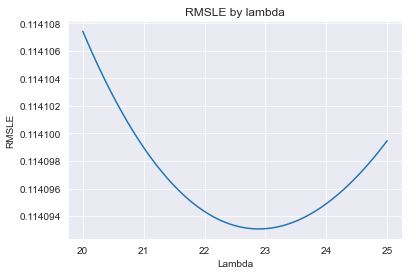
ridge = Ridge(alpha=22.9)

The Lasso Regression is
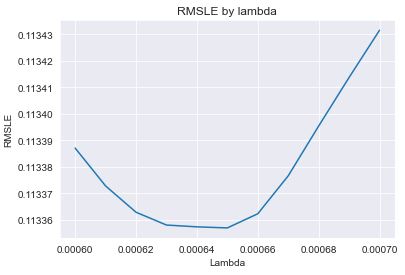
lambda_list = list(np.linspace(0.0006, 0.0007, 11))
rmsle_lasso = [
getRMSLE(Lasso(alpha=lambda_, max_iter=100000)) for lambda_ in lambda_list
]
rmsle_lasso = pd.Series(rmsle_lasso, index=lambda_list)

rmsle_lasso.plot(title=”RMSLE by lambda”)
plt.xlabel(“Lambda”)
plt.ylabel(“RMSLE”)
plt.savefig(“ameslassolambdarmsle.png”)
print(“Best lambda:”, rmsle_lasso.idxmin())
print(“RMSLE:”, rmsle_lasso.min())

Best lambda: 0.00065
RMSLE: 0.11335701578061286

lasso = Lasso(alpha=0.00065, max_iter=100000)

let’s apply the XGBoost algorithm
from xgboost import XGBRegressor

xgb = XGBRegressor(learning_rate=0.05,
n_estimators=2100,
max_depth=2,
min_child_weight=2,
gamma=0,
subsample=0.65,
colsample_bytree=0.46,
nthread=-1,
scale_pos_weight=1,
reg_alpha=0.464,
reg_lambda=0.8571,
silent=1,
random_state=7,
n_jobs=2)
getRMSLE(xgb)

0.11606096335909163

Let’s apply the LightGBM algorithm
from lightgbm import LGBMRegressor
lgb = LGBMRegressor(objective=’regression’,
learning_rate=0.05,
n_estimators=730,
num_leaves=8,
min_data_in_leaf=4,
max_depth=3,
max_bin=55,
bagging_fraction=0.78,
bagging_freq=5,
feature_fraction=0.24,
feature_fraction_seed=9,
bagging_seed=9,
min_sum_hessian_in_leaf=11)
getRMSLE(lgb)

0.11579673967953394

let’s design the average model

from sklearn.base import BaseEstimator, RegressorMixin, TransformerMixin, clone

class AveragingModel(BaseEstimator, RegressorMixin, TransformerMixin):
def init(self, models):
self.models = models

def fit(self, X, y):
    # Create clone models
    self.models_ = [clone(x) for x in self.models]

    # Train cloned models
    for model in self.models_:
        model.fit(X, y)

    return self

def predict(self, X):
    # Get predictions from trained clone models
    predictions = np.column_stack(
        [model.predict(X) for model in self.models_])

    # Return average predictions
    return np.mean(predictions, axis=1)

avg_model = AveragingModel(models=(ridge, lasso, xgb, lgb))
getRMSLE(avg_model)

0.1106991374718241

Let’s compare the X-plots

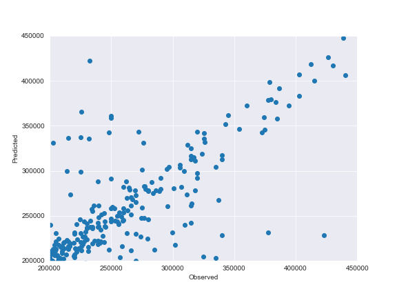
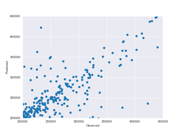
We can see that both XGBoost and LightGBM methods result in relatively similar X-plots and corresponding RMSLEs.

Case 4: MA

Let’s visualize ML model performance using Scikit-Plot evaluation metrics. The public dataset that we’ll use is the Boston housing price dataset. It has information about various houses of Boston and the price at which they were sold. We’ll divide it as well in train and test sets with the train_size=0.8 proportion. Let’s import libraries and import the data:

import scikitplot as skplt

import sklearn
from sklearn.datasets import load_boston
from sklearn.model_selection import train_test_split

from sklearn.ensemble import RandomForestClassifier, RandomForestRegressor, GradientBoostingClassifier, ExtraTreesClassifier
from sklearn.linear_model import LinearRegression, LogisticRegression
from sklearn.cluster import KMeans
from sklearn.decomposition import PCA

import matplotlib.pyplot as plt

import sys
import warnings
warnings.filterwarnings(“ignore”)

print(“Scikit Plot Version : “, skplt.version)
print(“Scikit Learn Version : “, sklearn.version)
print(“Python Version : “, sys.version)

%matplotlib inline

Scikit Plot Version :  0.3.7
Scikit Learn Version :  1.0.2
Python Version :  3.9.12 (main, Apr  4 2022, 05:22:27)

boston = load_boston()
X_boston, Y_boston = boston.data, boston.target

print(“Boston Dataset Size : “, X_boston.shape, Y_boston.shape)

print(“Boston Dataset Features : “, boston.feature_names)

Boston Dataset Size :  (506, 13) (506,)
Boston Dataset Features :  ['CRIM' 'ZN' 'INDUS' 'CHAS' 'NOX' 'RM' 'AGE' 'DIS' 'RAD' 'TAX' 'PTRATIO'
 'B' 'LSTAT']

X_boston_train, X_boston_test, Y_boston_train, Y_boston_test = train_test_split(X_boston, Y_boston,
train_size=0.8,
random_state=1)

print(“Boston Train/Test Sizes : “,X_boston_train.shape, X_boston_test.shape, Y_boston_train.shape, Y_boston_test.shape)

Boston Train/Test Sizes :  (404, 13) (102, 13) (404,) (102,)

Let’s plot the cross-validation performance of ML models by passing it the Boston dataset. Scikit-plot provides a method named plot_learning_curve() as a part of the estimators module which accepts estimator, X, Y, cross-validation info, and scoring metric for plotting performance of cross-validation on the dataset.

skplt.estimators.plot_learning_curve(LinearRegression(), X_boston, Y_boston,
cv=7, shuffle=True, scoring=”r2″, n_jobs=-1,
figsize=(6,4), title_fontsize=”large”, text_fontsize=”large”,
title=”Boston Linear Regression Learning Curve “);
plt.savefig(“bostonlinreglearncurve.png”)

skplt.estimators.plot_learning_curve(RandomForestRegressor(), X_boston, Y_boston,
cv=7, shuffle=True, scoring=”r2″, n_jobs=-1,
figsize=(6,4), title_fontsize=”large”, text_fontsize=”large”,
title=”Boston RandomForestRegressor Learning Curve “);
plt.savefig(“bostonrandomforestlearncurve.png”)

from xgboost import XGBRegressor
skplt.estimators.plot_learning_curve(XGBRegressor(), X_boston, Y_boston,
cv=7, shuffle=True, scoring=”r2″, n_jobs=-1,
figsize=(6,4), title_fontsize=”large”, text_fontsize=”large”,
title=”Boston XGBRegressor Learning Curve “);
plt.savefig(“bostonxgboostlearncurve.png”)

from lightgbm import LGBMRegressor
skplt.estimators.plot_learning_curve(LGBMRegressor(), X_boston, Y_boston,
cv=7, shuffle=True, scoring=”r2″, n_jobs=-1,
figsize=(6,4), title_fontsize=”large”, text_fontsize=”large”,
title=”Boston LGBMRegressor Learning Curve “);
plt.savefig(“bostonlgbmlearncurve.png”)

from sklearn.linear_model import Ridge, Lasso
skplt.estimators.plot_learning_curve(Ridge(), X_boston, Y_boston,
cv=7, shuffle=True, scoring=”r2″, n_jobs=-1,
figsize=(6,4), title_fontsize=”large”, text_fontsize=”large”,
title=”Boston Ridge Regression Learning Curve “);
plt.savefig(“bostonridgereglearncurve.png”)

skplt.estimators.plot_learning_curve(Lasso(), X_boston, Y_boston,
cv=7, shuffle=True, scoring=”r2″, n_jobs=-1,
figsize=(6,4), title_fontsize=”large”, text_fontsize=”large”,
title=”Boston Lasso Regression Learning Curve “);
plt.savefig(“bostonlassoreglearncurve.png”)

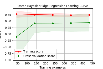
from sklearn import linear_model
reg = linear_model.BayesianRidge()
skplt.estimators.plot_learning_curve(reg, X_boston, Y_boston,
cv=7, shuffle=True, scoring=”r2″, n_jobs=-1,
figsize=(6,4), title_fontsize=”large”, text_fontsize=”large”,
title=”Boston BayesianRidge Regression Learning Curve “);
plt.savefig(“bostonBayesianRidgereglearncurve.png”)

from sklearn.linear_model import TweedieRegressor
reg = TweedieRegressor(power=1, alpha=0.5, link=’log’)
skplt.estimators.plot_learning_curve(reg, X_boston, Y_boston,
cv=7, shuffle=True, scoring=”r2″, n_jobs=-1,
figsize=(6,4), title_fontsize=”large”, text_fontsize=”large”,
title=”Boston TweedieRegressor Learning Curve “);
plt.savefig(“bostontweediereglearncurve.png”)

It is clear that RandomForestRegressor, XGBRegressor, and LGBMRegressor yield the best training and cross-validation scores for training examples > 420 compared to other ML algorithms.

Crucial Steps

• sssss
• ssss
• ssss
• ssss
• ssss
• ssss
• ssss

Key Takeaways

• We predict/estimate US house prices in order to allocate a valuation expert over a period of time.
• We need a fast AI to address rapidly increasing populations and the number of dwelling houses in the country.
• We use a region-dependent pre-trained ML model to predict prices of new houses.
• We import key Python libraries (pandas, scikit-learn, etc.) and download public-domain housing datasets from Kaggle or GitHub.
• We gather and clean, edit, scale and transform data so it can be used for model training and test predictions. Specifically, we identify the target variable (SalePrice), impute missing values, perform label encoding, standardization, splitting and (optional) balancing of training and testing datasets. For example, we can look at scatter plots to detect outliers to be dropped.
• The input data consists of a home’s features, including its eventual selling price and various descriptive features such as location, remodeling, age, size, type of sale (single family, commercial, etc).
• These features will be analyzed in determining a home’s value and what the shopper is most likely to buy.
• Feature engineering can determine what are the most important model features as there may be one feature that stands out or there may be several. Fore example, a larger living or basement area is linked to a higher house price.
• We perform model training using different linear and non-linear regression algorithms (Ridge, Lasso, Random Forest, Decision Treem SVM, XGBoost, etc.).
• The model performance is evaluated using a user-defined loss function (RMSE, MSE, OHMSE, etc.).
• The pre-trained model is then used to generate predictions for both training and validation inputs.
• Cross-validation of different ML algorithms has proven to be a suitable method to find an acceptable best fitting algorithm for the given set of features.
• It appears that location and square feet area play an important role in deciding the price of a property. This is helpful information for sellers and buyers.
• Results provide a primer on advanced ML real estate techniques as well as several best practices for ML readiness. 

Conclusions

Housing prices are an important reflection of the US real estate, and housing price ranges are of great interest for both buyers and sellers. Real estate is the world’s largest asset class, worthing $277 trillion, three times the total value of all publicly traded companies. And ML/AI applications have been accompanying its sector’s growth. 

One of the most popular AI applications in the industry is intelligent investing. This application helps answer questions like:

• Which house should I buy or build to maximize my return?
• Where or when should I do so?
• What is its optimum rent or sale price?

In this blog post, we have reviewed how ML leverages the power of housing data to tackle these important questions. We have also explored the pros and cons of ML algorithms and how optimizing various steps of actual Python workflows can help improve their performance.

References

Using Data to Predict Ames, Iowa Housing Price

Using linear regression and feature engineering to predict housing prices in Ames, Iowa

GitHub Rep Ames-housing-price-prediction

House-Price-Prediction-with-ML

Boston House Price Prediction Using Machine Learning

House Price Prediction using Linear Regression from Scratch

House price prediction – Austin, TX

GitHub 137 public repositories matching housing-prices

Predicting House Prices with Linear Regression | Machine Learning from Scratch (Part II)

California Housing Prices

California Housing

Machine Learning Project: House Price Prediction

Machine learning

About

Real Estate Supervised ML/AI Linear Regression Revisited – USA House Price Prediction

Supervised Machine Learning Use Case: Prediction of House Prices