This Python case example stems from the initial research into ML/AI wildfire prediction using the dataset that was downloaded from the UCI Machine Learning Repository.

Following the earlier study and the Github source, the entire supervised ML pipeline is implemented in Python/Jupyter as the following sequence of steps:
- Import required libraries
- Download input data
- Exploratory Data Analysis
- Feature Engineering
- Data Pre-Processing
- Data Scaling Transformation
- Training/Test Data Splitting
- Building Training Models
- Run RMSE/MAE Scores
- Final Model Comparison
Let’s set the working directory YOURPATH and import required libraries:
import os
os. getcwd()
os.chdir(‘YOURPATH’)
import numpy as np
import pandas as pd
import matplotlib.pyplot as plt
plt.style.use(‘seaborn’)
import seaborn as sns
from sklearn.preprocessing import LabelEncoder, StandardScaler, MinMaxScaler
from sklearn.model_selection import train_test_split
from sklearn.metrics import r2_score
import tensorflow as tensorflow
from keras.models import Sequential
from keras.layers import Dense, Dropout
from tensorflow import keras
from tensorflow.keras import layers
from tensorflow.keras.optimizers import SGD
from tensorflow.keras.utils import to_categorical
from keras.callbacks import EarlyStopping
from keras.callbacks import ModelCheckpoint
from keras.utils.vis_utils import plot_model
%matplotlib inline
#importing extra libraries
import matplotlib.pyplot as plt
import numpy as np
import pandas as pd
import seaborn as sns
from scipy.stats import norm
#Setting the figsize for a better vizualization
plt.rcParams[‘figure.figsize’]=(20,10)
from sklearn.model_selection import train_test_split
from sklearn.preprocessing import StandardScaler
from sklearn.model_selection import GridSearchCV
from sklearn.linear_model import LinearRegression
from sklearn.linear_model import Ridge
from sklearn.linear_model import Lasso
from sklearn.linear_model import ElasticNet
from sklearn.neighbors import KNeighborsRegressor
from sklearn.svm import SVR
from sklearn.tree import DecisionTreeRegressor
from sklearn.ensemble import RandomForestRegressor
from sklearn.ensemble import GradientBoostingRegressor
from sklearn.ensemble import ExtraTreesRegressor
from sklearn.metrics import mean_squared_error
from sklearn.metrics import mean_absolute_error
from scipy.sparse import hstack
import pickle
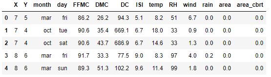
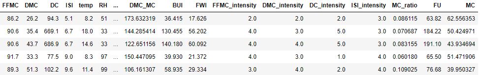
Let’s read the csv file
data = pd.read_csv(‘forestfires.csv’)
data.head(5)

Let’s check the overall percentile of the burned area
for i in range(0,100,10):
perc=np.percentile(data[‘area’],i)
print(‘area below {} percentile:’.format(i),perc)
area below 0 percentile: 0.0
area below 10 percentile: 0.0
area below 20 percentile: 0.0
area below 30 percentile: 0.0
area below 40 percentile: 0.0
area below 50 percentile: 0.52
area below 60 percentile: 2.0059999999999993
area below 70 percentile: 4.6339999999999995
area below 80 percentile: 8.822000000000001
area below 90 percentile: 25.262000000000043
Let’s create the scatter plot area(X,Y)
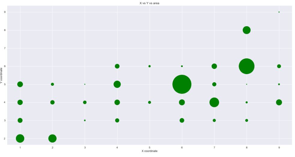
Creating the new feature X_Y by giving more importance to the X and Y coordinates associated with the relatively high percentage of the burned area
X_Y=[]
for i in range(len(data[‘Y’].values)):
if data[‘Y’][i]<7: new=0.6*data[‘X’][i]+0.4*data[‘Y’][i] X_Y.append(new) if data[‘Y’][i]>=7:
new=0.9data[‘X’][i]+0.1data[‘Y’][i]
X_Y.append(new)
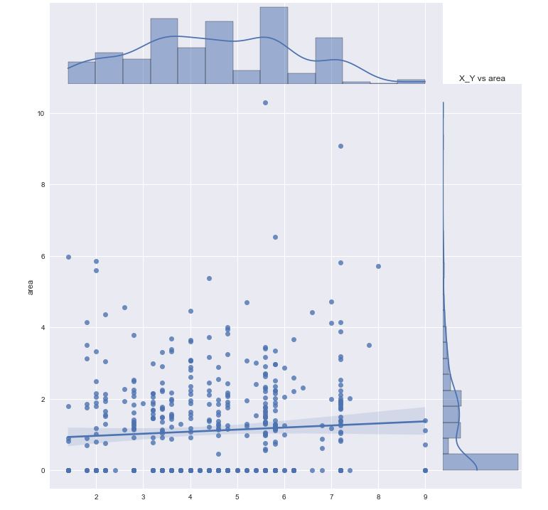
Let’s create the joint plot X_Y vs area
sns.jointplot(x=X_Y, y=np.cbrt(data[‘area’]),
kind=’reg’, space=0, size=10, ratio=5)
plt.xlabel(‘X_Y’)
plt.ylabel(‘area’)
plt.title(‘X_Y vs area’)
plt.show()
Let’s check the timing relationship area(month/day)
plt.scatter(x=data[‘month’],y=data[‘day’],s=data[‘area’]*5,c=’g’)
plt.xlabel(‘month’)
plt.ylabel(‘day’)
plt.title(‘month vs day vs area’)
plt.show()

Creating a new feature M_D
M_D=[]
for i in range(len(data[‘day’].values)):
#### Giving very less weightage to these months
if data['month'][i]=='jan'or data['month'][i]=='may' or data['month'][i]=='nov':
    M_D.append(np.random.normal(0.0,0.3,1)[0])

### Giving more weightage to these months
if data['month'][i]=='aug' or data['month'][i]=='sep':
    M_D.append(np.random.normal(0.7,1,1)[0])

### Giving moderate weightage to this month
if data['month'][i]=='jul':
    M_D.append(np.random.normal(0.6,0.7,1)[0])

### Giving less weightage to these months
if data['month'][i]=='feb' or data['month'][i]=='mar' or data['month'][i]=='apr' or data['month'][i]=='jun' or data['month'][i]=='oct' or data['month'][i]=='dec':
    M_D.append(np.random.normal(0.3,0.6,1)[0])
Let’s create the following M_D distance/density plot
sns.distplot(M_D,fit=norm)

and the joint plot area(M_D)
sns.jointplot(x=M_D, y=np.cbrt(data[‘area’]),
kind=’reg’, space=0, size=10, ratio=5)
plt.xlabel(‘M_D’)
plt.ylabel(‘area’)
plt.title(‘M_D vs area’)
plt.show()

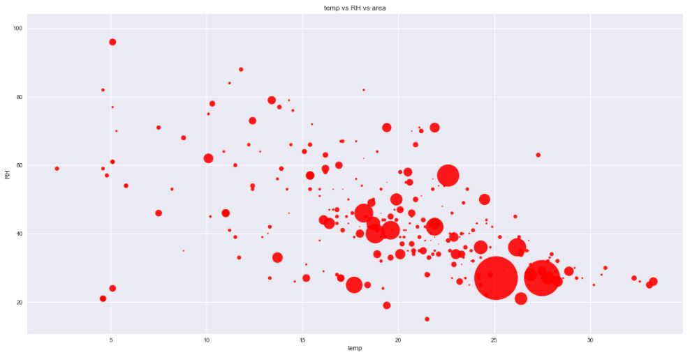
Checking the relationship between the fire area and the temperature and RH
plt.scatter(data[‘temp’], data[‘RH’], s=data[‘area’]*5, c=’r’,
alpha=0.9)
plt.xlabel(‘temp’)
plt.ylabel(‘RH’)
plt.title(‘temp vs RH vs area’)
Similarly, the relationship between the fire area and the temperature and wind is
plt.scatter(data[‘temp’], data[‘wind’], s=data[‘area’]*5, c=’r’,
alpha=0.9)
plt.xlabel(‘temp’)
plt.ylabel(‘wind’)
plt.title(‘temp vs wind vs area’)

Let’s check the new variable TRW
sns.jointplot(x=(data[‘temp’]0.4+data[‘RH’]0.4+data[‘wind’]*0.20), y=np.cbrt(data[‘area’]),
kind=’reg’, space=0, size=10, ratio=5)
plt.xlabel(‘TRW’)
plt.ylabel(‘area’)
plt.title(‘TRW vs area’)
plt.show()

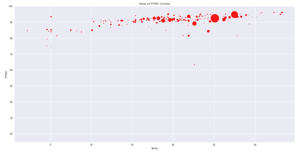
Let’s reate the scatter plot area vs temp and FFMC
plt.scatter(data[‘temp’], data[‘FFMC’], s=data[‘area’], c=’r’,
alpha=0.9)
plt.xlabel(‘temp’)
plt.ylabel(‘FFMC’)
plt.title(‘temp vs FFMC vs area’)
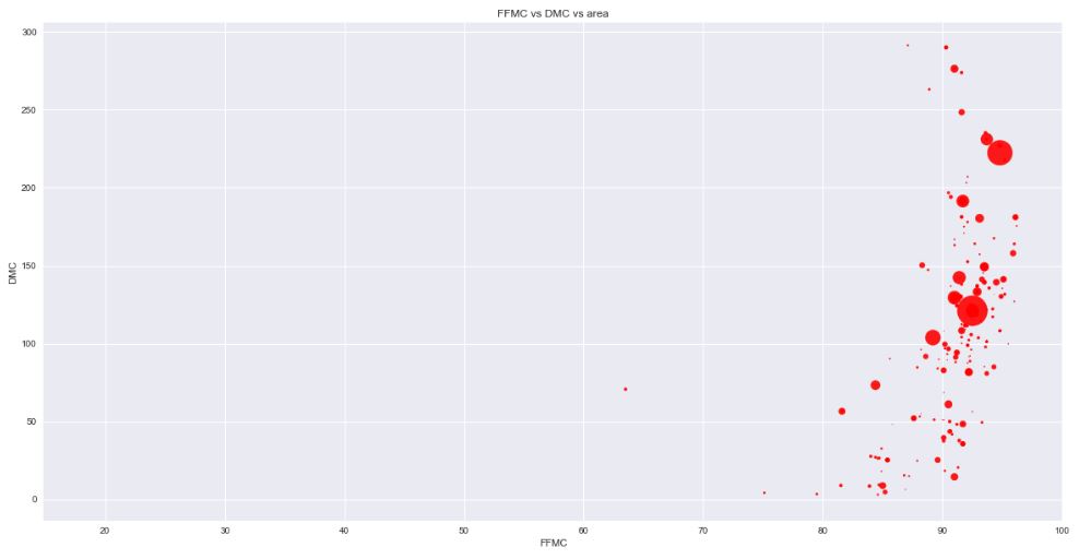
Let’s look at the scatter plot temp vs FFMC & DMC
plt.scatter(data[‘FFMC’], data[‘DMC’], s=data[‘area’], c=’r’,
alpha=0.9)
plt.xlabel(‘FFMC’)
plt.ylabel(‘DMC’)
plt.title(‘FFMC vs DMC vs area’)
Let’s sns plot and compare distributions of different area transformations
Creating subplots with 4 rows and one column
fig,(ax1,ax2,ax3,ax4)=plt.subplots(4,1,figsize=(20,30))
sns.distplot(data[‘area’],fit=norm,ax=ax1) ## Plotting the distributon of original values of area
ax1.set_title(‘original_dist’)
sns.distplot(np.log(data[‘area’]+1),fit=norm,ax=ax2) ## Plotting the distributon of Log transformed values of area
ax2.set_title(‘log_transform’)
sns.distplot(np.sqrt(data[‘area’]),fit=norm,ax=ax3) ## Plotting the distributon of Sqrt transformed values of area
ax3.set_title(‘sqrt_transform’)
sns.distplot(np.cbrt(data[‘area’]),fit=norm,ax=ax4) ## Plotting the distributon of Cbrt transformed values of area
ax4.set_title(‘cbrt_transform’)


Adding the cube root transformed area value column (best transformation) to the data
data[‘area_cbrt’]=np.cbrt(data[‘area’])
data.head()
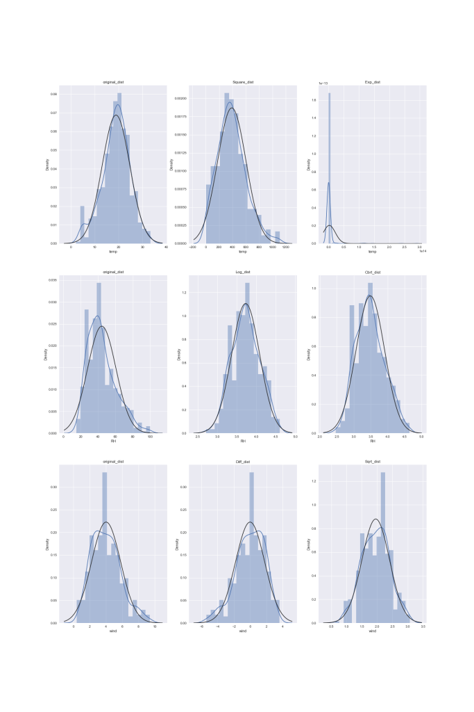
Let’s check distributions of other features and their transformations
Checking which transformation is best by plotting and comparing the distributions
Creating subplots with 3 rows and 3 columns
fig,axes=plt.subplots(3,3,figsize=(20,30))
Plotting the original distributon of temp
sns.distplot(data[‘temp’],fit=norm,ax=axes[0][0])
axes[0][0].set_title(‘original_dist’)
Applying Square,exponential Transformations
Plotting the Square,exp distributons of temp
sns.distplot(np.square(data[‘temp’]),fit=norm,ax=axes[0][1])
axes[0][1].set_title(‘Square_dist’)
sns.distplot(np.exp(data[‘temp’]),fit=norm,ax=axes[0][2])
axes[0][2].set_title(‘Exp_dist’)
Plotting the original distributon of RH
sns.distplot(data[‘RH’],fit=norm,ax=axes[1][0])
axes[1][0].set_title(‘original_dist’)
Plotting the Log, Cbrt distributons of RH
sns.distplot(np.log(data[‘RH’]),fit=norm,ax=axes[1][1])
axes[1][1].set_title(‘Log_dist’)
sns.distplot(np.cbrt(data[‘RH’]),fit=norm,ax=axes[1][2])
axes[1][2].set_title(‘Cbrt_dist’)
Plotting the original distributon of wind
sns.distplot(data[‘wind’],fit=norm,ax=axes[2][0])
axes[2][0].set_title(‘original_dist’)
Plotting the difference distributons of wind
sns.distplot((np.median(data[‘wind’])-data[‘wind’]),fit=norm,ax=axes[2][1])
axes[2][1].set_title(‘Diff_dist’)
sqrt yields better results than cbrt
Plotting the sqrt distribution of wind
sns.distplot(np.sqrt(data[‘wind’]),fit=norm,ax=axes[2][2])
axes[2][2].set_title(‘Sqrt_dist’)
plt.savefig(‘distributions_temp_wind_exp.png’)
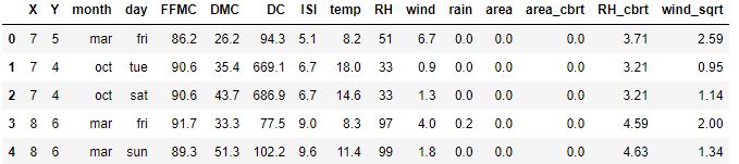
Adding the transformed values of weather indices to the data
data[‘RH_cbrt’]=np.cbrt(data[‘RH’]).round(2)
data[‘wind_sqrt’]=np.sqrt(data[‘wind’]).round(2)
data.head()
Let’s plot the transformed weather data
fig,axes=plt.subplots(2,2,figsize=(20,10))
init_col=[‘RH’,’wind’]
tran_col=[‘RH_cbrt’,’wind_sqrt’]
for i in range(2):
for j in range(2):
if i==0:
axes[i][j].scatter(data[init_col[j]],data[‘area’])
axes[i][j].set_title(init_col[j] + ‘vs’ + ‘area’)
axes[i][j].set_xlabel(init_col[j])
axes[i][j].set_ylabel(‘area’)
    if i==1:
        axes[i][j].scatter(data[tran_col[j]],data['area_cbrt'])
        axes[i][j].set_title(tran_col[j] + 'vs' + 'area_cbrt')
        axes[i][j].set_xlabel(tran_col[j])
        axes[i][j].set_ylabel('area_cbrt')

        plt.savefig('data_area_data_transform.png')

Let’s check distributions of other FWI features and their transformations.
Creating subplots with 4 rows and 3 columns
fig,axes=plt.subplots(4,3,figsize=(20,30))
Plotting the original distributon of FFMC
sns.distplot(data[‘FFMC’],fit=norm,ax=axes[0][0])
axes[0][0].set_title(‘original_dist’)
Plotting Square,exp distributons of FFMC
sns.distplot(np.square(data[‘FFMC’]),fit=norm,ax=axes[0][1])
axes[0][1].set_title(‘Square_dist’)
sns.distplot(np.exp(data[‘FFMC’]),fit=norm,ax=axes[0][2])
axes[0][2].set_title(‘Exp_dist’)
Plotting the original distributons of DMC
sns.distplot(data[‘DMC’],fit=norm,ax=axes[1][0])
axes[1][0].set_title(‘original_dist’)
Plotting Log,Cbrt distributons of DMC
sns.distplot(np.log(data[‘DMC’]),fit=norm,ax=axes[1][1])
axes[1][1].set_title(‘Log_dist’)
sns.distplot(np.cbrt(data[‘DMC’]),fit=norm,ax=axes[1][2])
axes[1][2].set_title(‘Cbrt_dist’)
Plotting the original distributon of DC
sns.distplot(data[‘DC’],fit=norm,ax=axes[2][0])
axes[2][0].set_title(‘original_dist’)
Plotting distributons of Square,cbrt Transformations of DC
sns.distplot(np.square(data[‘DC’]),fit=norm,ax=axes[2][1])
axes[2][1].set_title(‘Square_dist’)
sns.distplot(np.cbrt(data[‘DC’]),fit=norm,ax=axes[2][2])
axes[2][2].set_title(‘cbrt_dist’)
Plotting the original distributon of ISI
sns.distplot(data[‘ISI’],fit=norm,ax=axes[3][0])
axes[3][0].set_title(‘original_dist’)
Plotting distributons of Log,Cbrt Transformations of ISI
sns.distplot(np.log(data[‘ISI’]+1),fit=norm,ax=axes[3][1])
axes[3][1].set_title(‘log_dist’)
sns.distplot(np.cbrt(data[‘ISI’]),fit=norm,ax=axes[3][2])
axes[3][2].set_title(‘cbrt_dist’)
plt.savefig(‘distributions_fwi_transform.png’)

Creating New Features
Creating new feature X_Y
data[‘X_Y’]=X_Y
Creating new feature M_D
data[‘M_D’]=M_D
We have already seen in above plots the contribution of temp,rh and wind
Creating the new feature TRW=0.55*temp+0.3*RH+0.15*wind
data[‘TRW’]=data[‘temp’]0.4+0.4data[‘RH’]+0.2*data[‘wind’]
FFMC is linked to the moisture content (MC) of litter which is the initial layer of ground upto a depth of 5cm
MC=147.2(101-FFMC)/(59.5+FFMC)
data[‘FFMC_MC’]=(147.2*(101-data[‘FFMC’]))/(59.5+data[‘FFMC’])
DMC describes the MC=exp[(DMC-244.7)/-43.4]+20) of the Duff layer which is the beneath the litter up to a depth of 5 cm to 10 cm
data[‘DMC_MC’]=np.exp((data[‘DMC’]-244.7)/(-43.4))+20
BUI is the fire behaviour index
BUI is the linear combination of DMC and DC dominated by DMC, i.e. BUI=0.85DMC+0.15DC
data[‘BUI’]=0.85data[‘DMC’]+0.15data[‘DC’]
FWI is the linear combination of ISI and BUI
data[‘FWI’]=0.6data[‘ISI’]+0.4data[‘BUI’]
the fire intensity based on the FFMC value
Let’s create the moisture content ratio MC_ratio as FFMC_MC/DMC_MC
data[‘MC_ratio’]=data[‘FFMC_MC’]/data[‘DMC_MC’]
Let’s create the fuel code FU and MC as the linear combinations
data[‘FU’]=data[‘FFMC’]0.4+0.4data[‘DMC’]+0.2*data[‘DC’]
data[‘MC’]=data[‘FFMC_MC’]0.7+0.3data[‘DMC_MC’]
print(data.shape)
data.head()
in addition to
| X | Y | month | day |
|---|
Fire Intensity Ranking
Let’s perform the fire intensity ranking based on the FFMC value
0-80 Low, Rank=1
81-87 moderate, Rank=2
88-90 High, Rank=3
91-92 Very High, Rank=4
93+ Extreme, Rank=5
data.loc[(data.FFMC.round()>=0) & (data.FFMC.round()<=80),’FFMC_intensity’]=1 data.loc[(data.FFMC.round()>=81) & (data.FFMC.round()<=87),’FFMC_intensity’]=2 data.loc[(data.FFMC.round()>=88) & (data.FFMC.round()<=90),’FFMC_intensity’]=3 data.loc[(data.FFMC.round()>=91) & (data.FFMC.round()<=92),’FFMC_intensity’]=4 data.loc[(data.FFMC.round()>=93) ,’FFMC_intensity’]=5
Let’s consider the DMC_intensity ranking
data.loc[(data.DMC.round()>=0) & (data.DMC.round()<=12),’DMC_intensity’]=1 data.loc[(data.DMC.round()>=13) & (data.DMC.round()<=27),’DMC_intensity’]=2 data.loc[(data.DMC.round()>=28) & (data.DMC.round()<=41),’DMC_intensity’]=3 data.loc[(data.DMC.round()>=42) & (data.DMC.round()<=62),’DMC_intensity’]=4 data.loc[(data.DMC.round()>=63) ,’DMC_intensity’]=5
and the DC_intensity ranking
data.loc[(data[‘ISI’].round()>=0) & (data[‘ISI’].round()<=1.9),’ISI_intensity’]=1 data.loc[(data[‘ISI’].round()>=1.9) & (data[‘ISI’].round()<=4.9),’ISI_intensity’]=2 data.loc[(data[‘ISI’].round()>=5.0) & (data[‘ISI’].round()<=7.9),’ISI_intensity’]=3 data.loc[(data[‘ISI’].round()>=8.0) & (data[‘ISI’].round()<=10.9),’ISI_intensity’]=4 data.loc[(data[‘ISI’].round()>=11) ,’ISI_intensity’]=5
Feature Engineering
Let’s calculate feature correlations
import matplotlib.pyplot as plt
plt.figure(figsize = (16,10))
corr = data.corr()
sns.heatmap(corr,annot=True)
plt.savefig(‘heatmapcorr.png’, dpi=300, bbox_inches=’tight’)

Let’s print out sorted correlation values of area_cbrt
print(corr[“area_cbrt”].sort_values(ascending=False))
area_cbrt         1.000000
area              0.645930
BUI               0.084785
DC_intensity      0.084707
FU                0.084435
FWI               0.082552
temp              0.079305
DMC               0.078905
DC                0.076716
X_Y               0.070266
X                 0.070197
wind_sqrt         0.059054
wind              0.057859
FFMC              0.057257
DMC_intensity     0.050774
Y                 0.045406
MC_ratio          0.043133
FFMC_intensity    0.033511
ISI_intensity     0.027158
rain              0.016706
M_D               0.007781
ISI               0.000054
TRW              -0.037683
FFMC_MC          -0.057742
RH_cbrt          -0.060131
RH               -0.064098
DMC_MC           -0.073696
MC               -0.078477
Name: area_cbrt, dtype: float64
Let’s transform the features
data[‘log_FFMC_MC’]=np.log(data[‘FFMC_MC’])
data[‘log_DMC_MC’]=np.log(data[‘DMC_MC’])
data[‘log_MC_ratio’]=np.log(data[‘MC_ratio’])
while deleting the original data columns
col=[‘RH’,’wind’,’area’,’FFMC_MC’,’DMC_MC’,’MC_ratio’,’ISI’,’FWI’,’FU’,’MC’,’X’,’Y’]
data_final=data.drop(col,axis=1)
print(data_final.shape)
print(data_final.head())
print(data_final.isna().sum())
(517, 21)
  month  day  FFMC   DMC     DC  temp  rain  area_cbrt  RH_cbrt  wind_sqrt  \
0   mar  fri  86.2  26.2   94.3   8.2   0.0        0.0     3.71       2.59
1   oct  tue  90.6  35.4  669.1  18.0   0.0        0.0     3.21       0.95
2   oct  sat  90.6  43.7  686.9  14.6   0.0        0.0     3.21       1.14
3   mar  fri  91.7  33.3   77.5   8.3   0.2        0.0     4.59       2.00
4   mar  sun  89.3  51.3  102.2  11.4   0.0        0.0     4.63       1.34

   ...       M_D    TRW      BUI  FFMC_intensity  DMC_intensity  DC_intensity  \
0  ...  1.144798  25.02   36.415             2.0            2.0           2.0
1  ...  0.618729  20.58  130.455             4.0            3.0           5.0
2  ...  0.979240  19.30  140.180             4.0            4.0           5.0
3  ...  0.954346  42.92   39.930             4.0            3.0           1.0
4  ...  1.477790  44.52   58.935             3.0            4.0           2.0

   ISI_intensity  log_FFMC_MC  log_DMC_MC  log_MC_ratio
0            3.0     2.704870    5.156940     -2.452070
1            3.0     2.322296    4.971793     -2.649497
2            3.0     2.322296    4.809344     -2.487048
3            4.0     2.203203    5.013611     -2.810408
4            4.0     2.448778    4.664960     -2.216182

[5 rows x 21 columns]
month             0
day               0
FFMC              0
DMC               0
DC                0
temp              0
rain              0
area_cbrt         0
RH_cbrt           0
wind_sqrt         0
X_Y               0
M_D               0
TRW               0
BUI               0
FFMC_intensity    0
DMC_intensity     0
DC_intensity      0
ISI_intensity     0
log_FFMC_MC       0
log_DMC_MC        0
log_MC_ratio      0
dtype: int64
Let’s perform mean date (the month and day featurs) encoding
mean_month=data_final.groupby(‘month’)[‘area_cbrt’].mean().round(3).to_dict()
mean_day=data_final.groupby(‘day’)[‘area_cbrt’].mean().round(3).to_dict()
data_final[‘month’]=data_final[‘month’].map(mean_month)
data_final[‘day’]=data_final[‘day’].map(mean_day)
print(mean_month,mean_day)
{'apr': 1.035, 'aug': 1.067, 'dec': 2.316, 'feb': 1.031, 'jan': 0.0, 'jul': 1.13, 'jun': 0.857, 'mar': 0.731, 'may': 1.688, 'nov': 0.0, 'oct': 0.841, 'sep': 1.273} {'fri': 0.949, 'mon': 1.076, 'sat': 1.248, 'sun': 1.093, 'thu': 1.041, 'tue': 1.22, 'wed': 1.143}
Saving this dictioary for later use
pickle.dump(mean_month,open(‘mean_month_area_cbrt’,’wb’))
pickle.dump(mean_day,open(‘mean_day_area_cbrt’,’wb’))
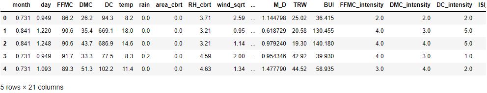
data_final.head()
| month | day | FFMC | DMC | DC | temp | rain | area_cbrt | RH_cbrt | wind_sqrt | … | M_D | TRW | BUI | FFMC_intensity | DMC_intensity | DC_intensity | ISI_intensity | log_FFMC_MC | log_DMC_MC | log_MC_ratio |
|---|
| 0.0 | 3.71 | 2.59 | … | 1.144798 | 25.02 | 36.415 | 2.0 | 2.0 | 2.0 | 3.0 | 2.704870 | 5.156940 | -2.452070 |
Checking the correlation between M_D and area_cbrt
col=[‘month’,’day’,’M_D’,’area_cbrt’]
corr=data[col].corr()
sns.heatmap(corr,annot=True)
plt.savefig(‘heatmapcorrmonthdayarea.png’, dpi=300, bbox_inches=’tight’)

The final data structure is
print(data_final.shape)
data_final.columns
(517, 21)
Index(['month', 'day', 'FFMC', 'DMC', 'DC', 'temp', 'rain', 'area_cbrt',
       'RH_cbrt', 'wind_sqrt', 'X_Y', 'M_D', 'TRW', 'BUI', 'FFMC_intensity',
       'DMC_intensity', 'DC_intensity', 'ISI_intensity', 'log_FFMC_MC',
       'log_DMC_MC', 'log_MC_ratio'],
      dtype='object')
Let’s save the data
data_final.to_csv(‘data_final’)
Scaled Data Preparation
Let’s read the data
data=pd.read_csv(‘data_final’)
Notice the new column “Unnamed” to be removed.
Standardizing the numerical values
def standardize(column):
scalar=StandardScaler()
column=scalar.fit_transform(column.reshape(-1,1))
return column,scalar
columns=list(data.columns)
columns.remove(‘area_cbrt’)
scalers_transform={}
for i in (columns):
data[i],scaler=standardize(data[i].values)
scalers_transform[i]=scaler
Saving these scalers for later use
pickle.dump(scalers_transform,open(‘scalers_transform’,’wb’))
Let’s check the scaling transform
scalers_transform
{'Unnamed: 0': StandardScaler(),
 'month': StandardScaler(),
 'day': StandardScaler(),
 'FFMC': StandardScaler(),
 'DMC': StandardScaler(),
 'DC': StandardScaler(),
 'temp': StandardScaler(),
 'rain': StandardScaler(),
 'RH_cbrt': StandardScaler(),
 'wind_sqrt': StandardScaler(),
 'X_Y': StandardScaler(),
 'M_D': StandardScaler(),
 'TRW': StandardScaler(),
 'BUI': StandardScaler(),
 'FFMC_intensity': StandardScaler(),
 'DMC_intensity': StandardScaler(),
 'DC_intensity': StandardScaler(),
 'ISI_intensity': StandardScaler(),
 'log_FFMC_MC': StandardScaler(),
 'log_DMC_MC': StandardScaler(),
 'log_MC_ratio': StandardScaler()}
Let’s delete the redundant column
del data[‘Unnamed: 0’]
and split the data into the training and testing datasets with test_size=0.15
X=data.drop(‘area_cbrt’,axis=1)
Y=data[‘area_cbrt’].values
x_train,x_test,y_train,y_test=train_test_split(X,Y,test_size=0.15)
Let’s look at the area statistics
data_final.area_cbrt.describe()
count    517.000000
mean       1.106882
std        1.399649
min        0.000000
25%        0.000000
50%        0.804145
75%        1.872931
max       10.294068
Name: area_cbrt, dtype: float64
Let’s begin with the contastant prediction area_cbrt1=1.1
y_pred_train=np.array([(area_cbrt1)**3 for i in range(y_train.shape[0])]) y_pred_test=np.array([(area_cbrt1)**3 for i in range(y_test.shape[0])])
Calculating the RMSE and MAE scores for this zero-order model
rmse_train_random=mean_squared_error((y_train)**3,(y_pred_train)**3,squared=False)
rmse_test_random=mean_squared_error((y_test)**3,(y_pred_test)**3,squared=False)
print(‘RMSE score for train data by a mean model:’, rmse_train_random)
print(‘RMSE score for test data by a mean model:’, rmse_test_random)
print(‘-‘*70)
mae_train_random=mean_absolute_error((y_train)**3,(y_pred_train)**3)
mae_test_random=mean_absolute_error((y_test)**3,(y_pred_test)**3)
print(‘MAE score for train data by a random model:’,mae_train_random)
print(‘MAE score for test data by a random model:’,mae_test_random)
RMSE score for train data by a mean model: 69.32858412079064
RMSE score for test data by a mean model: 21.989380793773037
----------------------------------------------------------------------
MAE score for train data by a mean model: 13.538765578776767
MAE score for test data by a mean model: 10.309375226589747
Let’s apply the linear regression
reg= LinearRegression()
reg.fit(x_train,y_train)
y_pred_train=reg.predict(x_train)
y_pred_test=reg.predict(x_test)
Calculating the RMSE scores
rmse_train_linear=mean_squared_error((y_train)**3,(y_pred_train)**3,squared=False)
rmse_test_linear=mean_squared_error((y_test)**3,(y_pred_test)**3,squared=False)
print(‘RMSE score for train data by a Linear regression model:’, rmse_train_linear)
print(‘RMSE score for test data by a Linear regression model:’, rmse_test_linear)
print(‘-‘*70)
Calculating MAE scores
mae_train_linear=mean_absolute_error((y_train)**3,(y_pred_train)**3)
mae_test_linear=mean_absolute_error((y_test)**3,(y_pred_test)**3)
print(‘MAE score for train data by a Linear regression model:’,mae_train_linear)
print(‘MAE score for test data by a Linear regression model:’,mae_test_linear)
pickle.dump(reg,open(‘lir_reg’,’wb’))
RMSE score for train data by a Linear regression model: 69.19699114969242
RMSE score for test data by a Linear regression model: 21.92818933571379
----------------------------------------------------------------------
MAE score for train data by a Linear regression model: 13.112736016498342
MAE score for test data by a Linear regression model: 9.927609872882762
Let’s apply the ridge regression
reg=Ridge()
params={‘alpha’:[10 ** x for x in range(-5, 5)]}
reg=GridSearchCV(estimator=reg,param_grid=params,scoring=’neg_root_mean_squared_error’)
reg.fit(x_train,y_train)
print(reg.best_params_)
reg=Ridge(alpha=reg.best_params_[‘alpha’])
reg.fit(x_train,y_train)
y_pred_train=reg.predict(x_train)
y_pred_test=reg.predict(x_test)
Calculating the RMSE scores
rmse_train_ridge=mean_squared_error((y_train)**3,(y_pred_train)**3,squared=False)
rmse_test_ridge=mean_squared_error((y_test)**3,(y_pred_test)**3,squared=False)
print(‘RMSE score for train data by a ridge regression model:’, rmse_train_ridge)
print(‘RMSE score for test data by a ridge regression model:’, rmse_test_ridge)
pickle.dump(reg,open(‘ridge_reg_rmse’,’wb’))
print(‘-‘*70)
reg=Ridge()
params={‘alpha’:[10 ** x for x in range(-5, 5)]}
reg=GridSearchCV(estimator=reg,param_grid=params,scoring=’neg_mean_absolute_error’)
reg.fit(x_train,y_train)
print(reg.best_params_)
reg=Ridge(alpha=reg.best_params_[‘alpha’])
reg.fit(x_train,y_train)
y_pred_train=reg.predict(x_train)
y_pred_test=reg.predict(x_test)
Calculating MAE scores
mae_train_ridge=mean_absolute_error((y_train)**3,(y_pred_train)**3)
mae_test_ridge=mean_absolute_error((y_test)**3,(y_pred_test)**3)
print(‘MAE score for train data by a ridge regression model:’,mae_train_ridge)
print(‘MAE score for test data by a ridge regression model:’,mae_test_ridge)
pickle.dump(reg,open(‘ridge_reg_mae’,’wb’))
{'alpha': 1000}
RMSE score for train data by a ridge regression model: 69.4313579792029
RMSE score for test data by a ridge regression model: 22.316358364598315
----------------------------------------------------------------------
{'alpha': 100}
MAE score for train data by a ridge regression model: 13.14786540926345
MAE score for test data by a ridge regression model: 9.914798621332315
Let’s apply the lasso regression
reg=Lasso()
params={‘alpha’:[10 ** x for x in range(-5, 5)]}
reg=GridSearchCV(estimator=reg,param_grid=params,scoring=’neg_root_mean_squared_error’)
reg.fit(x_train,y_train)
print(reg.best_params_)
reg=Lasso(alpha=reg.best_params_[‘alpha’])
reg.fit(x_train,y_train)
y_pred_train=reg.predict(x_train)
y_pred_test=reg.predict(x_test)
Calculating the RMSE scores
rmse_train_lasso=mean_squared_error((y_train)**3,(y_pred_train)**3,squared=False)
rmse_test_lasso=mean_squared_error((y_test)**3,(y_pred_test)**3,squared=False)
print(‘RMSE score for train data by a Lasso regression model:’, rmse_train_lasso)
print(‘RMSE score for test data by a Lasso regression model:’, rmse_test_lasso)
pickle.dump(reg,open(‘lasso_reg_rmse’,’wb’))
print(‘-‘*70)
reg=Lasso()
params={‘alpha’:[10 ** x for x in range(-5, 5)]}
reg=GridSearchCV(estimator=reg,param_grid=params,scoring=’neg_mean_absolute_error’)
reg.fit(x_train,y_train)
print(reg.best_params_)
reg=Lasso(alpha=reg.best_params_[‘alpha’])
reg.fit(x_train,y_train)
y_pred_train=reg.predict(x_train)
y_pred_test=reg.predict(x_test)
Calculating MAE scores
mae_train_lasso=mean_absolute_error((y_train)**3,(y_pred_train)**3)
mae_test_lasso=mean_absolute_error((y_test)**3,(y_pred_test)**3)
print(‘MAE score for train data by a Lasso regression model:’,mae_train_lasso)
print(‘MAE score for test data by a Lasso regression model:’,mae_test_lasso)
pickle.dump(reg,open(‘lasso_reg_mae’,’wb’))
{'alpha': 0.1}
RMSE score for train data by a Lasso regression model: 69.46749693840358
RMSE score for test data by a Lasso regression model: 22.304683983959
----------------------------------------------------------------------
{'alpha': 0.1}
MAE score for train data by a Lasso regression model: 13.217032831414896
MAE score for test data by a Lasso regression model: 10.133160454755082
Let’s apply the elastic net regression
reg=ElasticNet()
params={‘alpha’:[10 ** x for x in range(-5, 5)]}
reg=GridSearchCV(estimator=reg,param_grid=params,scoring=’neg_root_mean_squared_error’)
reg.fit(x_train,y_train)
print(reg.best_params_)
reg=ElasticNet(alpha=reg.best_params_[‘alpha’])
reg.fit(x_train,y_train)
y_pred_train=reg.predict(x_train)
y_pred_test=reg.predict(x_test)
Calculating the RMSE scores
rmse_train_elastic=mean_squared_error((y_train)**3,(y_pred_train)**3,squared=False)
rmse_test_elastic=mean_squared_error((y_test)**3,(y_pred_test)**3,squared=False)
print(‘RMSE score for train data by an elastic net model:’, rmse_train_elastic)
print(‘RMSE score for test data by an elastic net model:’, rmse_test_elastic)
pickle.dump(reg,open(‘elastic_reg_rmse’,’wb’)) #### Saving the model
print(‘-‘*70)
reg=ElasticNet()
params={‘alpha’:[10 ** x for x in range(-5, 5)]}
reg=GridSearchCV(estimator=reg,param_grid=params,scoring=’neg_mean_absolute_error’)
reg.fit(x_train,y_train)
print(reg.best_params_)
reg=ElasticNet(alpha=reg.best_params_[‘alpha’])
reg.fit(x_train,y_train)
y_pred_train=reg.predict(x_train)
y_pred_test=reg.predict(x_test)
Calculating MAE scores
mae_train_elastic=mean_absolute_error((y_train)**3,(y_pred_train)**3)
mae_test_elastic=mean_absolute_error((y_test)**3,(y_pred_test)**3)
print(‘MAE score for train data by an elastic net model:’,mae_train_elastic)
print(‘MAE score for test data by an elastic net model:’,mae_test_elastic)
pickle.dump(reg,open(‘elastic_reg_mae’,’wb’)) #### Saving the model
{'alpha': 0.1}
RMSE score for train data by an elastic net model: 69.40094343797868
RMSE score for test data by an elastic net model: 22.184657993566134
----------------------------------------------------------------------
{'alpha': 0.1}
MAE score for train data by an elastic net model: 13.18072127969128
MAE score for test data by an elastic net model: 10.052970826325032
Let’s apply the KNN Regressor
reg=KNeighborsRegressor()
params={‘n_neighbors’:[3,5,7,10,15,20,25,30,45,50,60,70,80,90,100,150,250,260,270,280,290,300]}
reg=GridSearchCV(estimator=reg,param_grid=params,scoring=’neg_root_mean_squared_error’)
reg.fit(x_train,y_train)
print(reg.best_params_)
reg=KNeighborsRegressor(n_neighbors=reg.best_params_[‘n_neighbors’])
reg.fit(x_train,y_train)
y_pred_train=reg.predict(x_train)
y_pred_test=reg.predict(x_test)
Calculating the RMSE scores
rmse_train_knn=mean_squared_error((y_train)**3,(y_pred_train)**3,squared=False)
rmse_test_knn=mean_squared_error((y_test)**3,(y_pred_test)**3,squared=False)
print(‘RMSE score for train data by a knn regressor model:’, rmse_train_knn)
print(‘RMSE score for test data by a knn regressor model:’, rmse_test_knn)
pickle.dump(reg,open(‘knn_reg_rmse’,’wb’)) #### Saving the model
print(‘-‘*70)
reg=KNeighborsRegressor()
params={‘n_neighbors’:[3,5,7,10,15,20,25,30,45,50,60,70,80,90,100,150,250,260,270,280,290,300]}
reg=GridSearchCV(estimator=reg,param_grid=params,scoring=’neg_mean_absolute_error’)
reg.fit(x_train,y_train)
print(reg.best_params_)
reg=KNeighborsRegressor(n_neighbors=reg.best_params_[‘n_neighbors’])
reg.fit(x_train,y_train)
y_pred_train=reg.predict(x_train)
y_pred_test=reg.predict(x_test)
Calculating the MAE scores
mae_train_knn=mean_absolute_error((y_train)**3,(y_pred_train)**3)
mae_test_knn=mean_absolute_error((y_test)**3,(y_pred_test)**3)
print(‘MAE score for train data by a knn regressor model:’, mae_train_knn)
print(‘MAE score for test data by a knn regressor model:’, mae_test_knn)
pickle.dump(reg,open(‘knn_reg_mae’,’wb’)) #### Saving the model
{'n_neighbors': 100}
RMSE score for train data by a knn regressor model: 69.41705968993003
RMSE score for test data by a knn regressor model: 22.326107622781123
----------------------------------------------------------------------
{'n_neighbors': 100}
MAE score for train data by a knn regressor model: 13.30646067903156
MAE score for test data by a knn regressor model: 10.241892886500835
Let’s apply the Decision Tree Regressor
reg=DecisionTreeRegressor(criterion=’mse’)
params={‘max_depth’:[3,5,7,10,15,20,25,30]}
reg=GridSearchCV(estimator=reg,param_grid=params,scoring=’neg_root_mean_squared_error’)
reg.fit(x_train,y_train)
print(reg.best_params_)
reg=DecisionTreeRegressor(criterion=’mse’,max_depth=reg.best_params_[‘max_depth’])
reg.fit(x_train,y_train)
y_pred_train=reg.predict(x_train)
y_pred_test=reg.predict(x_test)
Calculating the RMSE scores
rmse_train_dt=mean_squared_error((y_train)**3,(y_pred_train)**3,squared=False)
rmse_test_dt=mean_squared_error((y_test)**3,(y_pred_test)**3,squared=False)
print(‘RMSE score for train data by a decision tree regressor model:’, rmse_train_dt)
print(‘RMSE score for test data by a decision tree regressor model:’, rmse_test_dt)
pickle.dump(reg,open(‘dt_reg_rmse’,’wb’)) #### Saving the model
print(‘-‘*100)
reg=DecisionTreeRegressor(criterion=’mae’)
params={‘max_depth’:[3,5,7,10,15,20,25,30]}
reg=GridSearchCV(estimator=reg,param_grid=params,scoring=’neg_mean_absolute_error’)
reg.fit(x_train,y_train)
print(reg.best_params_)
reg=DecisionTreeRegressor(criterion=’mae’,max_depth=reg.best_params_[‘max_depth’])
reg.fit(x_train,y_train)
y_pred_train=reg.predict(x_train)
y_pred_test=reg.predict(x_test)
Calculating the MAE scores
mae_train_dt=mean_absolute_error((y_train)**3,(y_pred_train)**3)
mae_test_dt=mean_absolute_error((y_test)**3,(y_pred_test)**3)
print(‘MAE score for train data by a decision tree regressor model:’, mae_train_dt)
print(‘MAE score for test data by a decision tree regressor model:’, mae_test_dt)
pickle.dump(reg,open(‘dt_reg_mae’,’wb’)) #### Saving the model
{'max_depth': 3}
RMSE score for train data by a decision tree regressor model: 59.36451536225977
RMSE score for test data by a decision tree regressor model: 87.37196062413051
--------------------------------------------------------------------------
{'max_depth': 3}
MAE score for train data by a decision tree regressor model: 12.929088838268795
MAE score for test data by a decision tree regressor model: 10.025333139446646
Let’s apply the Random Forest Regressor
reg=RandomForestRegressor(criterion=’mse’)
params={‘n_estimators’:[10,20,30,50,100,500,1000]}
reg=GridSearchCV(estimator=reg,param_grid=params,scoring=’neg_root_mean_squared_error’)
reg.fit(x_train,y_train)
print(reg.best_params_)
reg=RandomForestRegressor(criterion=’mse’,n_estimators=reg.best_params_[‘n_estimators’])
reg.fit(x_train,y_train)
y_pred_train=reg.predict(x_train)
y_pred_test=reg.predict(x_test)
Calculating the RMSE scores
rmse_train_rf=mean_squared_error((y_train)**3,(y_pred_train)**3,squared=False)
rmse_test_rf=mean_squared_error((y_test)**3,(y_pred_test)**3,squared=False)
print(‘RMSE score for train data by a RandomForest regressor model:’, rmse_train_rf)
print(‘RMSE score for test data by a RandomForest regressor model:’, rmse_test_rf)
pickle.dump(reg,open(‘rf_reg_rmse’,’wb’)) #### Saving the model
print(‘-‘*70)
reg=RandomForestRegressor(criterion=’mae’)
params={‘n_estimators’:[10,20,30,50,100,500,1000]}
reg=GridSearchCV(estimator=reg,param_grid=params,scoring=’neg_mean_absolute_error’)
reg.fit(x_train,y_train)
print(reg.best_params_)
reg=RandomForestRegressor(criterion=’mae’,n_estimators=reg.best_params_[‘n_estimators’])
reg.fit(x_train,y_train)
y_pred_train=reg.predict(x_train)
y_pred_test=reg.predict(x_test)
Calculating the MAE scores
mae_train_rf=mean_absolute_error((y_train)**3,(y_pred_train)**3)
mae_test_rf=mean_absolute_error((y_test)**3,(y_pred_test)**3)
print(‘MAE score for train data by a RandomForest regressor model:’, mae_train_rf)
print(‘MAE score for test data by a RandomForest regressor model:’, mae_test_rf)
pickle.dump(reg,open(‘rf_reg_mae’,’wb’)) #### Saving the model
{'n_estimators': 1000}
RMSE score for train data by a RandomForest regressor model: 49.16034802325878
RMSE score for test data by a RandomForest regressor model: 22.361775374599215
----------------------------------------------------------------------
{'n_estimators': 500}
MAE score for train data by a RandomForest regressor model: 8.476428629063237
MAE score for test data by a RandomForest regressor model: 10.74416785250558
Let’s apply the GradientBoostingRegressor
reg=GradientBoostingRegressor()
params={‘n_estimators’:[10,20,30,50,100,500,1000]}
reg=GridSearchCV(estimator=reg,param_grid=params,scoring=’neg_root_mean_squared_error’)
reg.fit(x_train,y_train)
print(reg.best_params_)
reg=GradientBoostingRegressor(n_estimators=reg.best_params_[‘n_estimators’])
reg.fit(x_train,y_train)
y_pred_train=reg.predict(x_train)
y_pred_test=reg.predict(x_test)
Calculating the RMSE scores
rmse_train_gbdt=mean_squared_error((y_train)**3,(y_pred_train)**3,squared=False)
rmse_test_gbdt=mean_squared_error((y_test)**3,(y_pred_test)**3,squared=False)
print(‘RMSE score for train data by a GBDT regressor model:’, rmse_train_gbdt)
print(‘RMSE score for test data by a GBDT regressor model:’, rmse_test_gbdt)
pickle.dump(reg,open(‘gbdt_reg_rmse’,’wb’)) #### Saving the model
print(‘-‘*70)
reg=GradientBoostingRegressor()
params={‘n_estimators’:[10,20,30,50,100,500,1000]}
reg=GridSearchCV(estimator=reg,param_grid=params,scoring=’neg_mean_absolute_error’)
reg.fit(x_train,y_train)
print(reg.best_params_)
reg=GradientBoostingRegressor(n_estimators=reg.best_params_[‘n_estimators’])
reg.fit(x_train,y_train)
y_pred_train=reg.predict(x_train)
y_pred_test=reg.predict(x_test)
Calculating the MAE scores
mae_train_gbdt=mean_absolute_error((y_train)**3,(y_pred_train)**3)
mae_test_gbdt=mean_absolute_error((y_test)**3,(y_pred_test)**3)
print(‘MAE score for train data by a GBDT regressor model:’, mae_train_gbdt)
print(‘MAE score for test data by a GBDT regressor model:’, mae_test_gbdt)
pickle.dump(reg,open(‘gbdt_reg_mae’,’wb’)) #### Saving the model
{'n_estimators': 10}
RMSE score for train data by a GBDT regressor model: 65.55354517356737
RMSE score for test data by a GBDT regressor model: 22.752005211758735
----------------------------------------------------------------------
{'n_estimators': 10}
MAE score for train data by a GBDT regressor model: 12.743391810429754
MAE score for test data by a GBDT regressor model: 10.629013940106166
Let’s apply the ExtraTreesRegressor
reg=ExtraTreesRegressor(criterion=’mse’)
params={‘n_estimators’:[10,20,30,50,100,500,1000]}
reg=GridSearchCV(estimator=reg,param_grid=params,scoring=’neg_root_mean_squared_error’)
reg.fit(x_train,y_train)
print(reg.best_params_)
reg=ExtraTreesRegressor(criterion=’mse’,n_estimators=reg.best_params_[‘n_estimators’])
reg.fit(x_train,y_train)
y_pred_train=reg.predict(x_train)
y_pred_test=reg.predict(x_test)
Calculating the RMSE scores
rmse_train_et=mean_squared_error((y_train)3,(y_pred_train)3,squared=False)
rmse_test_et=mean_squared_error((y_test)3,(y_pred_test)3,squared=False)
print(‘RMSE score for train data by a Extra Tree regressor model:’, rmse_train_et)
print(‘RMSE score for test data by a Extra Tree regressor model:’, rmse_test_et)
pickle.dump(reg,open(‘et_reg_rmse’,’wb’)) #### Saving the model
print(‘-‘*70)
reg=ExtraTreesRegressor(criterion=’mae’)
params={‘n_estimators’:[10,20,30,50,100,500,1000]}
reg=GridSearchCV(estimator=reg,param_grid=params,scoring=’neg_mean_absolute_error’)
reg.fit(x_train,y_train)
print(reg.best_params_)
reg=ExtraTreesRegressor(criterion=’mae’,n_estimators=reg.best_params_[‘n_estimators’])
reg.fit(x_train,y_train)
y_pred_train=reg.predict(x_train)
y_pred_test=reg.predict(x_test)
Calculating the MAE scores
mae_train_et=mean_absolute_error((y_train)3,(y_pred_train)3)
mae_test_et=mean_absolute_error((y_test)3,(y_pred_test)3)
print(‘MAE score for train data by a Extra Tree regressor model:’, mae_train_et)
print(‘MAE score for test data by a Extra Tree regressor model:’, mae_test_et)
pickle.dump(reg,open(‘et_reg_mae’,’wb’)) #### Saving the model
{'n_estimators': 50}
RMSE score for train data by a Extra Tree regressor model: 1.6259798283965848e-13
RMSE score for test data by a Extra Tree regressor model: 25.884662790379124
----------------------------------------------------------------------
{'n_estimators': 1000}
MAE score for train data by a Extra Tree regressor model: 0.03086214584895277
MAE score for test data by a Extra Tree regressor model: 10.536791469743722
Let’s apply the XGBOOST algorithm
import xgboost as xg
Instantiation
xgb_r = xg.XGBRegressor(objective =’reg:linear’,
n_estimators = 10, seed = 123)
Fitting the model
xgb_r.fit(x_train,y_train)
y_pred_train=xgb_r.predict(x_train)
y_pred_test=xgb_r.predict(x_test)
Calculating the RMSE scores
rmse_train_xgb=mean_squared_error((y_train)**3,(y_pred_train)**3,squared=False)
rmse_test_xgb=mean_squared_error((y_test**)3,(y_pred_test)**3,squared=False)
print(‘RMSE score for train data by a Support Vector regressor model:’, rmse_train_xgb)
print(‘RMSE score for test data by a Support Vector regressor model:’, rmse_test_xgb)
Calculating the MAE scores
mae_train_xgb=mean_absolute_error((y_train)**3,(y_pred_train)**3)
mae_test_xgb=mean_absolute_error((y_test)**3,(y_pred_test)**3)
print(‘MAE score for train data by the xgb model:’, mae_train_xgb)
print(‘MAE score for test data by the xgb model:’, mae_test_xgb)
pickle.dump(reg,open(‘xgb_reg_mae’,’wb’)) #### Saving the model
RMSE score for train data by a Support Vector regressor model: 42.31588372249749
RMSE score for test data by a Support Vector regressor model: 24.670862330322198
MAE score for train data by the xgb model: 8.25194541823674
MAE score for test data by the xgb model: 11.69193135814189
Let’s apply the Support Vector Regressor
reg=SVR()
params={‘kernel’:[‘rbf’,’linear’,’poly’],’C’:[0.0001,0.001,0.01,0.1,1,10,100,1000]}
reg=GridSearchCV(estimator=reg,param_grid=params,scoring=’neg_root_mean_squared_error’)
reg.fit(x_train,y_train)
print(reg.best_params_)
reg=SVR(C=reg.best_params_[‘C’],kernel=reg.best_params_[‘kernel’])
reg.fit(x_train,y_train)
y_pred_train=reg.predict(x_train)
y_pred_test=reg.predict(x_test)
Calculating the RMSE scores
rmse_train_svr=mean_squared_error((y_train)**3,(y_pred_train)**3,squared=False)
rmse_test_svr=mean_squared_error((y_test)**3,(y_pred_test)**3,squared=False)
print(‘RMSE score for train data by a Support Vector regressor model:’, rmse_train_svr)
print(‘RMSE score for test data by a Support Vector regressor model:’, rmse_test_svr)
pickle.dump(reg,open(‘svr_reg_rmse’,’wb’)) #### Saving the model
print(‘-‘*70)
reg=SVR()
params={‘kernel’:[‘rbf’,’linear’,’poly’],’C’:[0.0001,0.001,0.01,0.1,1,10,100,1000]}
reg=GridSearchCV(estimator=reg,param_grid=params,scoring=’neg_mean_absolute_error’)
reg.fit(x_train,y_train)
print(reg.best_params_)
reg=SVR(C=reg.best_params_[‘C’],kernel=reg.best_params_[‘kernel’])
reg.fit(x_train,y_train)
y_pred_train=reg.predict(x_train)
y_pred_test=reg.predict(x_test)
Calculating the MAE scores
mae_train_svr=mean_absolute_error((y_train)**3,(y_pred_train)**3)
mae_test_svr=mean_absolute_error((y_test)**3,(y_pred_test)**3)
print(‘MAE score for train data by a Support Vector regressor model:’, mae_train_svr)
print(‘MAE score for test data by a Support Vector regressor model:’, mae_test_svr)
pickle.dump(reg,open(‘svr_reg_mae’,’wb’)) #### Saving the model
{'C': 0.01, 'kernel': 'linear'}
RMSE score for train data by a Support Vector regressor model: 69.59983289231299
RMSE score for test data by a Support Vector regressor model: 22.587171400062093
----------------------------------------------------------------------
{'C': 0.01, 'kernel': 'linear'}
MAE score for train data by a Support Vector regressor model: 13.09276829045713
MAE score for test data by a Support Vector regressor model: 10.18036738425034
Let’s look at the customized hybrid model by calling Custom_model()
def custom_model_train(samples,models):
trained_models=[]
for i in (models):               ### Training the each model with each 15 samples
    for j in (samples):
        x=j.drop('area_cbrt',axis=1)
        y=j['area_cbrt']


        i.fit(x,y)          ### Fitting the models
    trained_models.append(i)
return trained_models
Getting the k predictions from k models with data D2
def predictions_of_custom_model(Data,models):
x=Data.drop(‘area’,axis=1)
y=Data[‘area’]
predictions=[]
for i in (models):
predicted_y=i.predict(x)
predictions.append(predicted_y)
return predictions
def meta_model(D2_meta_train_x,D2_meta_train_y,test_meta_x,test_meta_y):
### Support Vector Regressor AS Meta model
reg=SVR()

params={'C':[0.0001,0.001,0.01,0.1,1,10,100,1000]}

reg=GridSearchCV(estimator=reg,param_grid=params,scoring='neg_root_mean_squared_error')

reg.fit(D2_meta_train_x,D2_meta_train_y)

print(reg.best_params_)

reg=SVR(C=reg.best_params_['C'])

reg.fit(D2_meta_train_x,D2_meta_train_y)

y_pred_train=reg.predict(D2_meta_train_x)
y_pred_test=reg.predict(test_meta_x)

### Calculating the RMSE scores

rmse_train_custom=mean_squared_error(D2_meta_train_y,y_pred_train,squared=False)
rmse_test_custom=mean_squared_error(test_meta_y,y_pred_test,squared=False)

print('RMSE score for train data by a custom model:', rmse_train_custom)
print('RMSE score for test data by a custom model:', rmse_test_custom)

pickle.dump(reg,open('custom_reg_rmse_nml','wb'))  #### Saving the model

print('-'*70)
reg=SVR()
params={'C':[0.0001,0.001,0.01,0.1,1,10,100,1000]}

reg=GridSearchCV(estimator=reg,param_grid=params,scoring='neg_mean_absolute_error')

reg.fit(D2_meta_train_x,D2_meta_train_y)

print(reg.best_params_)

reg=SVR(C=reg.best_params_['C'])

reg.fit(D2_meta_train_x,D2_meta_train_y)

y_pred_train=reg.predict(D2_meta_train_x)
y_pred_test=reg.predict(test_meta_x)

### Calculating the MAE scores

mae_train_custom=mean_absolute_error(D2_meta_train_y,y_pred_train)
mae_test_custom=mean_absolute_error(test_meta_y,y_pred_test)

print('MAE score for train data by a custom model:', mae_train_custom)
print('MAE score for test data by a custom model:', mae_test_custom)

pickle.dump(reg,open('custom_reg_mae_nml','wb'))  #### Saving the model

return rmse_train_custom,rmse_test_custom,mae_train_custom,mae_test_custom
import random
def Custom_model(Data):
### Splitting the data in to train and test
train,test=train_test_split(Data,test_size=0.2)
### Splitting the  train in to D1 and D2

D1,D2=train_test_split(train,test_size=0.5)

### Creating 15 samples from the data D1


samples=[]   ### Creating the smaples list

rows=[i for i in range(D1.shape[0])]

for i in range(15):
    sample=random.choices(rows,k=150)  ### Selecting the indexes with replacement
    sample=D1.iloc[sample]              ## Creating the new sample

    samples.append(sample)

#### Defining the custom model

### Initiating the models

LIR=LinearRegression()
Ridg=Ridge()
Laso=Lasso()
Elastic=ElasticNet()
KNN=KNeighborsRegressor()
DT=DecisionTreeRegressor()
RF=RandomForestRegressor()
GBDT=GradientBoostingRegressor()
Extra=ExtraTreesRegressor()
XGBoost=xgb.XGBRegressor()
SVM=SVR()

models=[LIR,Ridg,Laso,Elastic,KNN,DT,RF,GBDT,Extra,XGBoost,SVM]

trained_models=custom_model_train(samples,models)  ### Getting the trained models

#### Getting the predictions of D2
predictions_k=predictions_of_custom_model(D2,trained_models)

### Creating training dataset for meta model
D2_meta_train_x=pd.DataFrame(data=predictions_k,index=models).T  ### Creating a dataset with the k predictions from k models
D2_meta_train_y=D2['area_cbrt']  ### Target values for meta model training

#### Creating the testing data for meta model

test_predictions_k=predictions_of_custom_model(test,trained_models)

test_meta_x=pd.DataFrame(data=test_predictions_k,index=models).T  ### Creating a dataset with the k predictions from k models
test_meta_y=test['area_cbrt']  ### Target values for meta model testing


rmse_train_custom,rmse_test_custom,mae_train_custom,mae_test_custom=meta_model(D2_meta_train_x,D2_meta_train_y,test_meta_x,test_meta_y)

return rmse_train_custom,rmse_test_custom,mae_train_custom,mae_test_custom
Rmse_train_custom_nml,Rmse_test_custom_nml,Mae_train_custom_nml,Mae_test_custom_nml=Custom_model(data)
{'n_estimators': 10}
RMSE score for train data by a custom model: 66.0281887406213
RMSE score for test data by a custom model: 11.90786400739486
-------------------------------------------------------------------------
{'n_estimators': 30}
MAE score for train data by a custom model: 16.445680959668845
MAE score for test data by a custom model: 7.865120210656043
Summary
!pip install prettytable
Collecting prettytable
Comparing the results of all models
from prettytable import PrettyTable
ptable = PrettyTable()
ptable.title = ” Model Comparision “
ptable.field_names = [“Model”,’RMSE_score’,’MAE_Score’]
ptable.add_row([“Random model”,rmse_test_random,mae_test_random])
ptable.add_row([“Linear Regression”,rmse_test_linear,mae_test_linear])
ptable.add_row([“Ridge Regression”,rmse_test_ridge,mae_test_ridge])
ptable.add_row([“Lasso Regression”,rmse_test_lasso,mae_test_lasso])
ptable.add_row([“Elastic net Regression”,rmse_test_elastic,mae_test_elastic])
ptable.add_row([“KNN Regression”,rmse_test_knn,mae_test_knn])
ptable.add_row([“Decision Tree Regression”,rmse_test_dt,mae_test_dt])
ptable.add_row([“Random Forest Regression”,rmse_test_rf,mae_test_rf])
ptable.add_row([“GBDT Regression”,rmse_test_gbdt,mae_test_gbdt])
ptable.add_row([“Extra Trees Regression”,rmse_test_et,mae_test_et])
ptable.add_row([“XGBoost Regression”,rmse_test_xgb,mae_test_xgb])
ptable.add_row([“Support vector Regression”,rmse_test_svr,mae_test_svr])
ptable.add_row([“Custom model”,Rmse_test_custom,Mae_test_custom])
print(ptable)
+---------------------------------------------------------------------+
|                          Model Comparision                          |
+---------------------------+--------------------+--------------------+
|           Model           |     RMSE_score     |     MAE_Score      |
+---------------------------+--------------------+--------------------+
|        Random model       | 21.989380793773037 | 10.309375226589747 |
|     Linear Regression     | 21.92818933571379  | 9.927609872882762  |
|      Ridge Regression     | 22.316358364598315 | 9.914798621332315  |
|      Lasso Regression     |  22.304683983959   | 10.133160454755082 |
|   Elastic net Regression  | 22.184657993566134 | 10.052970826325032 |
|       KNN Regression      | 22.326107622781123 | 10.241892886500835 |
|  Decision Tree Regression | 87.37196062413051  | 10.025333139446646 |
|  Random Forest Regression | 22.361775374599215 | 10.524664487939804 |
|      GBDT Regression      | 22.752005211758735 | 10.629013940106166 |
|   Extra Trees Regression  | 21.982166544843334 | 10.325457483153489 |
|     XGBoost Regression    | 24.670862330322198 | 11.69193135814189  |
| Support vector Regression | 22.587171400062093 | 10.18036738425034  |
|        Custom model       | 11.90786400739486  | 7.865120210656043  |
+---------------------------+--------------------+--------------------+
We can see that the custom meta training model yields the best RMS and MAE scores. This is because the custom model initiates training models using all available algorithms
LIR=LinearRegression()
Ridg=Ridge()
Laso=Lasso()
Elastic=ElasticNet()
KNN=KNeighborsRegressor()
DT=DecisionTreeRegressor()
RF=RandomForestRegressor()
GBDT=GradientBoostingRegressor()
Extra=ExtraTreesRegressor()
XGBoost=xgb.XGBRegressor()
SVM=SVR()
in combination with data random sampling (by creating 20 samples from the data itself).
In addition to deep learning algorithms, we can invoke hyperparameter tuning within the NN framework, as suggested by the earlier study and the follow-up pilot project.


Leave a comment