AI-Powered Stroke Prediction

Contents:

Introduction

Stroke, also known as brain attack, happens when blood flow to the brain is blocked, preventing it from getting oxygen and nutrients from it and causing the death of brain cells within minutes. According to the World Health Organization (WHO) stroke is the 2nd leading cause of death globally after ischemic heart disease, responsible for approximately 11% of total deaths. Stroke victims can experience paralysis, impaired speed, or loss of vision. While some of the Stroke risk factors cannot be modified, such as family history of cerebrovascular diseases, age, gender and race, others can and are estimated to account for 60% -80% of stroke risk in the general population.

Therefore, predicting stroke outcome for new cases can be determining for them to be treated early enough and avoid disabling and mortal consequences.

The use of AI-powered Machine Learning (ML) techniques in medical records have great impact on the fields of healthcare and bio-medicine [1-4]. This assists the medical practitioners to identify the onset of disease at an earlier stage. Here, we are particularly interested in stroke, and to identify the key factors that are associated with its occurrence.

In this blog, we formulate the ML stroke prediction process as a binary classification problem and provide a detailed understanding of the various risk factors for stroke prediction. Specifically, we analyse various features present in Electronic Health Record (EHR) records of patients, and identify the most important factors necessary for stroke prediction [1,2]. In doing so, we use dimensionality reduction techniques to identify patterns in low-dimension subspace of the feature space [1-4]. We benchmark popular ML/AI binary classification models for stroke prediction in a publicly available dataset.

Key Steps

Our ML stroke prediction workflow [1-3] in Python consists of the 7 steps

that implement ETL Preparation + ML Execution + Performance QC + Prediction:

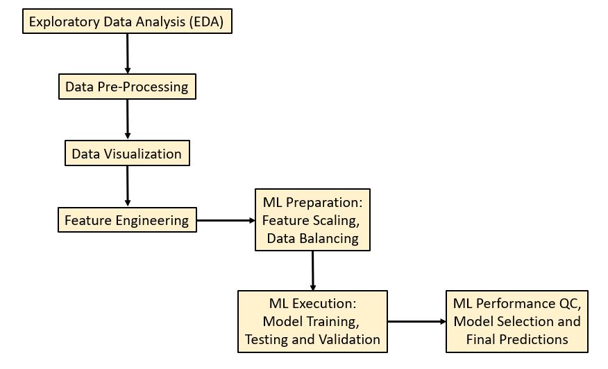
**Key elements of the ML stroke prediction algorithm**

This boils down to the following sequence:

Install the Anaconda IDE with the Jupyter notebook and Python 3.9.
Install and import the required Python ML libraries.
Read input EMR Kaggle dataset healthcare-dataset-stroke-data.csv
Input data preparation, editing, transformation and visualization
Feature engineering, correlations and impact factors
Train/test data splitting (test_size=0.25) and SMOTE balancing
Binary classification model training, ML benchmarking, testing and X-validation
Scikit-Plot: Visualizing ML Algorithm Results & Performance
Output the final classification report, the best training model and predictions

Importing Libraries

Let’s begin with importing/installing the required libraries:

!pip install imblearn

!pip install xgboost

!pip install tensorflow

import pandas as pd
import numpy as np
import matplotlib.pyplot as plt
import seaborn as sns
from sklearn.preprocessing import LabelEncoder
from sklearn.feature_selection import SelectKBest, f_classif
from sklearn.model_selection import train_test_split
from sklearn.metrics import accuracy_score, f1_score,classification_report,precision_score,recall_score
from imblearn.over_sampling import SMOTE/SMOTENC
from sklearn.linear_model import LogisticRegression
from sklearn.ensemble import RandomForestClassifier
from sklearn.svm import SVC
from xgboost import XGBClassifier

from sklearn.preprocessing import StandardScaler
from sklearn.decomposition import PCA
from sklearn.pipeline import make_pipeline

import tensorflow as tf
from tensorflow.keras.wrappers.scikit_learn import KerasClassifier
from sklearn.model_selection import cross_val_score

Reading Input Data

data=pd.read_csv(‘YOURPATH/healthcare-dataset-stroke-data.csv’)

df=data
data.head(10)

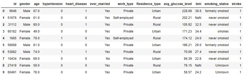
Displaying top 10 rows

data.info()

<class 'pandas.core.frame.DataFrame'>
RangeIndex: 5110 entries, 0 to 5109
Data columns (total 12 columns):
 #   Column             Non-Null Count  Dtype  
---  ------             --------------  -----  
 0   id                 5110 non-null   int64  
 1   gender             5110 non-null   object 
 2   age                5110 non-null   float64
 3   hypertension       5110 non-null   int64  
 4   heart_disease      5110 non-null   int64  
 5   ever_married       5110 non-null   object 
 6   work_type          5110 non-null   object 
 7   Residence_type     5110 non-null   object 
 8   avg_glucose_level  5110 non-null   float64
 9   bmi                4909 non-null   float64
 10  smoking_status     5110 non-null   object 
 11  stroke             5110 non-null   int64  
dtypes: float64(3), int64(4), object(5)
memory usage: 479.2+ KB

Showing information about dataset

data.describe()

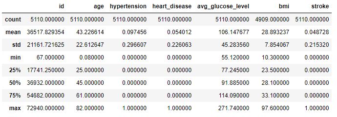
Showing data’s statistical features.

We can print the table out as follows:

print(stroke_df.shape)
print(stroke_df.head(10))
print(stroke_df.describe().T)

(5110, 12)
      id  gender   age  hypertension  heart_disease ever_married  \
0   9046    Male  67.0             0              1          Yes   
1  51676  Female  61.0             0              0          Yes   
2  31112    Male  80.0             0              1          Yes   
3  60182  Female  49.0             0              0          Yes   
4   1665  Female  79.0             1              0          Yes   
5  56669    Male  81.0             0              0          Yes   
6  53882    Male  74.0             1              1          Yes   
7  10434  Female  69.0             0              0           No   
8  27419  Female  59.0             0              0          Yes   
9  60491  Female  78.0             0              0          Yes   

       work_type Residence_type  avg_glucose_level   bmi   smoking_status  \
0        Private          Urban             228.69  36.6  formerly smoked   
1  Self-employed          Rural             202.21   NaN     never smoked   
2        Private          Rural             105.92  32.5     never smoked   
3        Private          Urban             171.23  34.4           smokes   
4  Self-employed          Rural             174.12  24.0     never smoked   
5        Private          Urban             186.21  29.0  formerly smoked   
6        Private          Rural              70.09  27.4     never smoked   
7        Private          Urban              94.39  22.8     never smoked   
8        Private          Rural              76.15   NaN          Unknown   
9        Private          Urban              58.57  24.2          Unknown   

   stroke  
0       1  
1       1  
2       1  
3       1  
4       1  
5       1  
6       1  
7       1  
8       1  
9       1  
                    count          mean           std    min        25%  \
id                 5110.0  36517.829354  21161.721625  67.00  17741.250   
age                5110.0     43.226614     22.612647   0.08     25.000   
hypertension       5110.0      0.097456      0.296607   0.00      0.000   
heart_disease      5110.0      0.054012      0.226063   0.00      0.000   
avg_glucose_level  5110.0    106.147677     45.283560  55.12     77.245   
bmi                4909.0     28.893237      7.854067  10.30     23.500   
stroke             5110.0      0.048728      0.215320   0.00      0.000   

                         50%       75%       max  
id                 36932.000  54682.00  72940.00  
age                   45.000     61.00     82.00  
hypertension           0.000      0.00      1.00  
heart_disease          0.000      0.00      1.00  
avg_glucose_level     91.885    114.09    271.74  
bmi                   28.100     33.10     97.60  
stroke                 0.000      0.00      1.00

As we can see, the Kaggle stroke dataset has 11 variables representing clinical features for predicting stroke events plus 1 record ID (columns) and 5110 observations (rows). This dataset is used to predict whether a patient is likely to get stroke based on the input parameters like gender, age, various diseases, and smoking status. Each row in the data provides relavant information about the patient.

Exploratory Data Analysis (EDA)

The Gender attribute states the gender of the patient. Let’s see how does Gender affects and Gender wise comparison of stroke rate.

print(‘Unique values\n’,data[‘gender’].unique())

print(‘Value Counts\n’,data[‘gender’].value_counts())

Above codes will help to give us information about it’s unique values and count of each value.

sns.countplot(data=data,x=’gender’)

Helps to plot a count plot which will help us to see count of values in each unique category.

sns.countplot(data=data,x=’gender’,hue=’stroke’)

This plot will help to analyze how gender will affect chances of stroke.

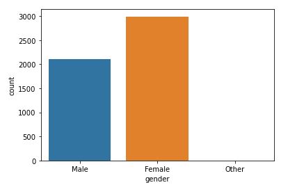
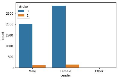
The dataset appears to be imbalanced. As we can there is not much difference between stroke rate concerning gender.

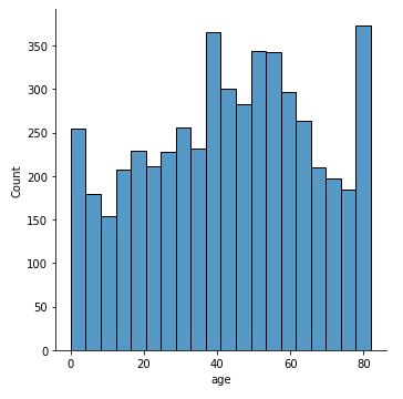
Let’s look at the Age attribute.

data[‘age’].nunique()

Returns number of unique values in this attribute

sns.displot(data[‘age’])

This will plot a distribution plot of variable age

plt.figure(figsize=(15,7))
sns.boxplot(data=data,x=’stroke’,y=’age’)

Above code will plot a boxplot of variable age with respect of target attribute stroke

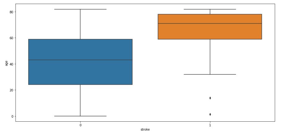
One can see that 60+ seniors tend to have a high risk of stroke. Some outliers can be seen for young people who suffer from stroke.

Since hypertension (high blood pressure) might lead to stroke, we consider the Hypertension attribute as well.

print(‘Unique values\n’,data[‘hypertension’].unique())
print(‘Value Counts\n’,data[‘hypertension’].value_counts())

Above codes will help to give us information about it’s unique values and count of each value.

sns.countplot(data=data,x=’hypertension’)

Helps to plot a count plot which will help us to see count of values in each unique category.

sns.countplot(data=data,x=’hypertension’,hue=’stroke’)

This plot will help to analyze how gender will affect chances of stroke.

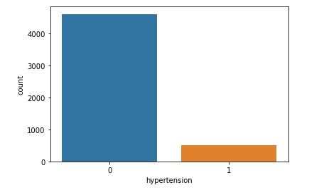
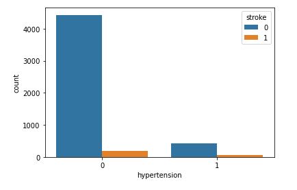
Even though hypertension can cause a stroke, our dataset does not contain a large amount clinical records of patients with high blood pressure.

Let’s look at heart disease associated with a higher risk of stroke.

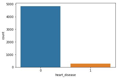
print(‘Unique Value\n’,data[‘heart_disease’].unique())
print(‘Value Counts\n’,data[‘heart_disease’].value_counts())

Above code will return unique value for heart disease attribute and its value counts

sns.countplot(data=data,x=’heart_disease’)

Will plot a counter plot of variable heart diseases

sns.countplot(data=data,x=’heart_disease’,hue=’stroke’)

This plot will help to analyze how gender will affect chances of stroke.

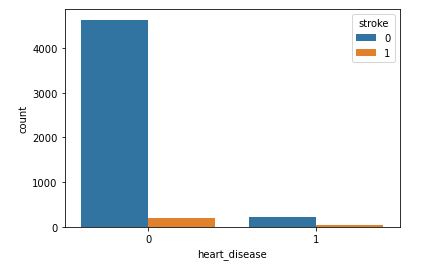
As with hypertension, it’s rather difficult to estimate the impact of heart desease because the number of recorded stroke patients with heart desease is relatively small.

The “ever_married” attribute will tell us whether or not the patient was ever married.

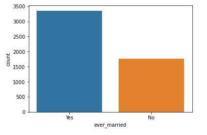
print(‘Unique Values\n’,data[‘ever_married’].unique())
print(‘Value Counts\n’,data[‘ever_married’].value_counts())

Above code will show us number unique values of attribute and its count

sns.countplot(data=data,x=’ever_married’)

Counter plot of ever married attribute

sns.countplot(data=data,x=’ever_married’,hue=’stroke’)

Ever married with respect to stroke

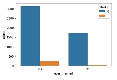
It is clear that people who are married have a higher stroke rate.

Let’s check the relationship between working conditions and the risk of stroke.

print(‘Unique Value\n’,data[‘work_type’].unique())
print(‘Value Counts\n’,data[‘work_type’].value_counts())

Above code will return unique values of attributes and its count

sns.countplot(data=data,x=’work_type’)

Above code will create a count plot

sns.countplot(data=data,x=’work_type’,hue=’stroke’)

Above code will create a count plot with respect to stroke

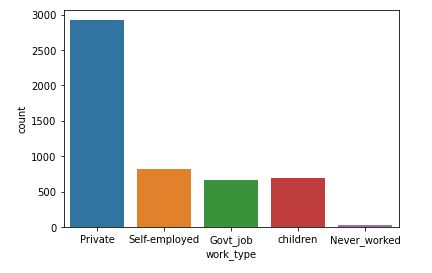
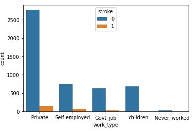
People working in the Private sector have a highest risk of stroke.

Let’s look at the residence type of stroke patients (urban or rural).

print(‘Unique Values\n’,data[‘Residence_type’].unique())
print(“Value Counts\n”,data[‘Residence_type’].value_counts())

Above code will return unique values of variable and its count

sns.countplot(data=data,x=’Residence_type’)

This will create a counter plot

sns.countplot(data=data,x=’Residence_type’,hue=’stroke’)

Residence Type with respect to stroke

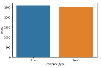
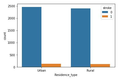
This attribute is of no use for stroke prediction. It would be best to discard it.

Let’s examine the average glucose level of stroke patients.

data[‘avg_glucose_level’].nunique()

Number of unique values

sns.displot(data[‘avg_glucose_level’])

Distribution of avg_glucose_level

sns.boxplot(data=data,x=’stroke’,y=’avg_glucose_level’)

Avg_glucose_level and Stroke

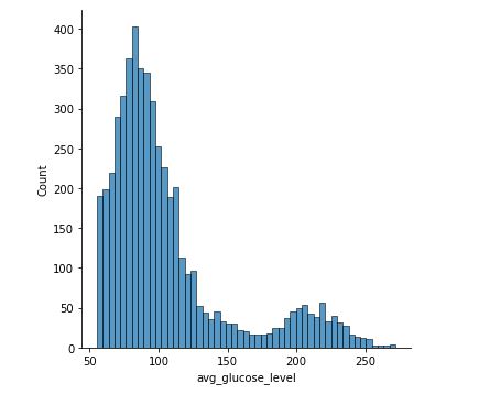
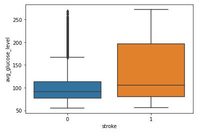
We can see that people having stroke have an average glucose level of more than 100.

Body Mass Index (BMI) is a measure of body fat based on height and weight of adult men and women. Let’s see how does it affect the chances of having a stroke.

data[‘bmi’].fillna(data[‘bmi’].mean(),inplace=True)

Filling null values with average value

data[‘bmi’].nunique()

Returns number of unique values in that attribute

sns.displot(data[‘bmi’])

Distribution of BMI

sns.boxplot(data=data,x=’stroke’,y=’bmi’)

BMI with respect to Stroke

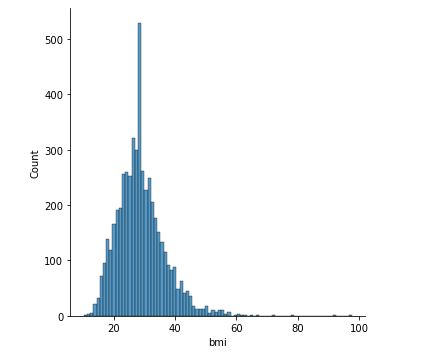
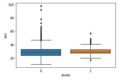
The relationship between BMI and stroke is unclear at this stage due to the overlap of two box plots.

Let’s check the impact of smoking.

print(‘Unique Values\n’,data[‘smoking_status’].unique())
print(‘Value Counts\n’,data[‘smoking_status’].value_counts())

Returns unique values and its count

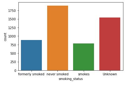
sns.countplot(data=data,x=’smoking_status’)

sns.countplot(data=data,x=’smoking_status’,hue=’stroke’)

Smoking Status with respect to Stroke

print(‘Unique Value\n’,data[‘stroke’].unique())
print(‘Value Counts\n’,data[‘stroke’].value_counts())

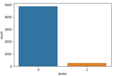
sns.countplot(data=data,x=’stroke’)

Count Plot of Stroke

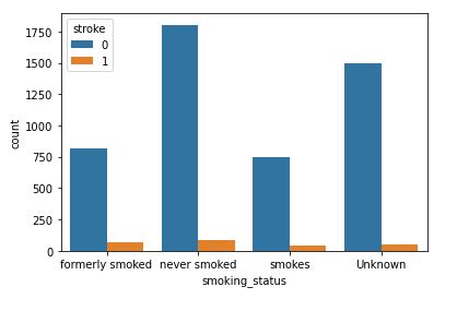
As with BMI, the correlation between the smoking status and the risk of stroke is unclear at this stage.

Finally, let’ plot our target binary variable Stroke.

print(‘Unique Value\n’,data[‘stroke’].unique())
print(‘Value Counts\n’,data[‘stroke’].value_counts())

sns.countplot(data=data,x=’stroke’)

Count Plot of Stroke

Here is the summary of attribute unique values:

Gender

Unique values
['Male' 'Female' 'Other']
Value Counts
Female    2994
Male      2115
Other        1

Age

Number of Unique Values:

Hypertension

Value Count [0 1]
Value Counts
0 4612
1 498

Unique Values and Value Counts:

Heart Disease

Unique Value
[1 0]
Value Counts
0    4834
1     276

Ever Married

Unique Values
['Yes' 'No']
Value Counts
Yes    3353
No     1757

Work Type

Unique Value
['Private' 'Self-employed' 'Govt_job' 'children' 'Never_worked']
Value Counts
Private          2925
Self-employed     819
children          687
Govt_job          657
Never_worked       22

Residence Type

Unique Values
['Urban' 'Rural']
Value Counts
Urban    2596
Rural    2514

Average Glucose Level

Unique Values and Count:

BMI

Null Values:

Unique Values and Counts:

Smoking Status

Unique Values
['formerly smoked' 'never smoked' 'smokes' 'Unknown']
Value Counts
never smoked       1892
Unknown            1544
formerly smoked     885
smokes              789

Stroke

Unique Value
[1 0]
Value Counts
0    4861
1     249

Feature Engineering

Let’s encode our categorical data into numeric ones using Label Encoder.

cols=data.select_dtypes(include=[‘object’]).columns
print(cols)

This code will fetch columns whose data type is object.

le=LabelEncoder()

Initializing our Label Encoder object

data[cols]=data[cols].apply(le.fit_transform)

Transfering categorical data into numeric

print(data.head(10))

Index(['gender', 'ever_married', 'work_type', 'Residence_type',
       'smoking_status'],
      dtype='object')
   gender   age  hypertension  heart_disease  ever_married  work_type  \
0       1  67.0             0              1             1          2   
1       0  61.0             0              0             1          3   
2       1  80.0             0              1             1          2   
3       0  49.0             0              0             1          2   
4       0  79.0             1              0             1          3   
5       1  81.0             0              0             1          2   
6       1  74.0             1              1             1          2   
7       0  69.0             0              0             0          2   
8       0  59.0             0              0             1          2   
9       0  78.0             0              0             1          2   

   Residence_type  avg_glucose_level        bmi  smoking_status  stroke  
0               1             228.69  36.600000               1       1  
1               0             202.21  28.893237               2       1  
2               0             105.92  32.500000               2       1  
3               1             171.23  34.400000               3       1  
4               0             174.12  24.000000               2       1  
5               1             186.21  29.000000               1       1  
6               0              70.09  27.400000               2       1  
7               1              94.39  22.800000               2       1  
8               0              76.15  28.893237               0       1  
9               1              58.57  24.200000               0       1

Let’s compute the feature correlation matrix

plt.figure(figsize=(15,10))
sns.heatmap(data.corr(),annot=True,fmt=’.2′)

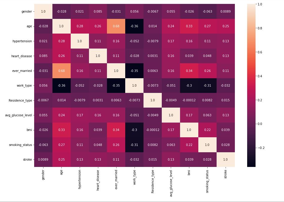
Variables that exhibit weak correlations are:

age, hypertension, heart_disease, ever_married, and avg_glucose_level.

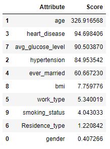
Let’s double check our observations using SelectKBest and F_Classif.

classifier = SelectKBest(score_func=f_classif,k=5)
fits = classifier.fit(data.drop(‘stroke’,axis=1),data[‘stroke’])
x=pd.DataFrame(fits.scores_)
columns = pd.DataFrame(data.drop(‘stroke’,axis=1).columns)
fscores = pd.concat([columns,x],axis=1)
fscores.columns = [‘Attribute’,’Score’]
fscores.sort_values(by=’Score’,ascending=False)

import matplotlib.pyplot as plt
fscores.columns = [‘Attribute’,’Score’]
fscores.sort_values(by=’Score’,ascending=False)

naming the x and y axis

f = plt.figure()
f.set_figwidth(16)
f.set_figheight(4)
plt.xlabel(‘Features’)
plt.ylabel(‘ML/AI Importance Factor’)
plt.plot(fscores[‘Attribute’],fscores[‘Score’])
plt.show()

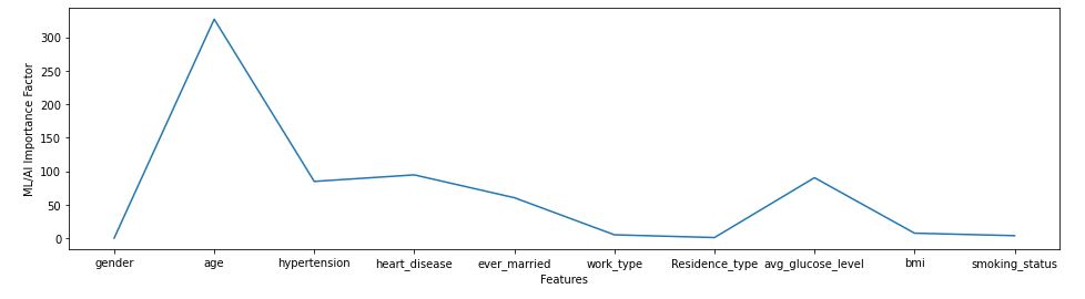
cols=fscores[fscores[‘Score’]>50][‘Attribute’]
print(cols)

1                  age
2         hypertension
3        heart_disease
4         ever_married
7    avg_glucose_level
Name: Attribute, dtype: object

Data Preparation

ID is nothing but a unique number assigned to every patient to keep track of them and making them unique. So we can remove it.

data.drop("id",inplace=True,axis=1)

I can see there are 201 NaN values for BMI variable. I decide to impute values for BMI since there are 40 patients who had a stroke that have a missing BMI value. The median was chosen over the mean since BMI has a long right tail.

stroke_df.fillna(stroke_df.median(), inplace=True)
stroke_df

The categorical data set is then transformed prior to processing through algorithms. Features with only 2 values were transformed into 1s and 0s using class mapping: ever_married, Residence_type, gender. Features with more than 2 values were transformed using One-Hot Label Encoding with the built-in Pandas get_dummies function: work_type, smoking_status.

# transform nominal variables that only have 2 values
class_mapping = {label: idx for idx, label in enumerate(np.unique(stroke_df['ever_married']))}
print(class_mapping)stroke_df['ever_married'] = stroke_df['ever_married'].map(class_mapping)
class_mapping = {label: idx for idx, label in enumerate(np.unique(stroke_df['Residence_type']))}
print(class_mapping)stroke_df['Residence_type'] = stroke_df['Residence_type'].map(class_mapping)
class_mapping = {label: idx for idx, label in enumerate(np.unique(stroke_df['gender']))}
print(class_mapping)stroke_df['gender'] = stroke_df['gender'].map(class_mapping)# transform nominal variables that have more than 2 values
stroke_df[['work_type','smoking_status']] = stroke_df[['work_type','smoking_status']].astype(str)# concatenate the nominal variables from pd.getdummies and the ordinal variables to form the final datasettranspose = pd.get_dummies(stroke_df[['work_type','smoking_status']])
stroke_dummies_df = pd.concat([stroke_df,transpose],axis=1)[['id','age','hypertension','heart_disease','ever_married','Residence_type','avg_glucose_level','bmi','gender','work_type_Govt_job','work_type_Never_worked','work_type_Private','work_type_Self-employed','work_type_children','smoking_status_Unknown','smoking_status_formerly smoked','smoking_status_never smoked','smoking_status_smokes','stroke']]
stroke_dummies_df

Now, let’s split features into training and testing sets for training and testing our classification models.

train_x,test_x,train_y,test_y=train_test_split(data[cols],data['stroke'],random_state=1255,test_size=0.25)
#Splitting data
train_x.shape,test_x.shape,train_y.shape,test_y.shape
# Shape of data
((3832, 5), (1278, 5), (3832,), (1278,))

Let’s balance our training and test data. We are going to use the SMOTE method

smote=SMOTE()
train_x,train_y=smote.fit_resample(train_x,train_y)
test_x,test_y=smote.fit_resample(test_x,test_y)

print(train_x.shape,train_y.shape,test_x.shape,test_y.shape)

(7296, 5) (7296,) (2426, 5) (2426,)

Model Building, Testing and X-Validation

Let’s models using Logistic Regression, Random Forest Classifier, SVM, and XGBClassifier. We select the best model performer XGBClassifier while comparing other ML algorithms.

xgc=XGBClassifier(objective=’binary:logistic’,n_estimators=100000,max_depth=5,learning_rate=0.001,n_jobs=-1)
xgc.fit(train_x,train_y)
predict=xgc.predict(test_x)
print(‘Accuracy –> ‘,accuracy_score(predict,test_y))
print(‘F1 Score –> ‘,f1_score(predict,test_y))
print(‘Classification Report –> \n’,classification_report(predict,test_y))

Accuracy -->  0.9117889530090684
F1 Score -->  0.9066317626527051
Classification Report  --> 
               precision    recall  f1-score   support

           0       0.97      0.87      0.92      1347
           1       0.86      0.96      0.91      1079

    accuracy                           0.91      2426
   macro avg       0.91      0.92      0.91      2426
weighted avg       0.92      0.91      0.91      2426

Model Predictions and Performance QC

Let’s examine the model performance using scikit-plot

!pip install scikit-plot

import scikitplot as skplt

mport sklearn
from sklearn.datasets import load_digits, load_boston, load_breast_cancer
from sklearn.model_selection import train_test_split

from sklearn.ensemble import RandomForestClassifier, RandomForestRegressor, GradientBoostingClassifier, ExtraTreesClassifier
from sklearn.linear_model import LinearRegression, LogisticRegression
from sklearn.cluster import KMeans
from sklearn.decomposition import PCA

import matplotlib.pyplot as plt

import sys
import warnings
warnings.filterwarnings(“ignore”)

print(“Scikit Plot Version : “, skplt.version)
print(“Scikit Learn Version : “, sklearn.version)
print(“Python Version : “, sys.version)

%matplotlib inline

Scikit Plot Version :  0.3.7
Scikit Learn Version :  1.0.2
Python Version :  3.9.12 (main, Apr  4 2022, 05:22:27) [MSC v.1916 64 bit (AMD64)]

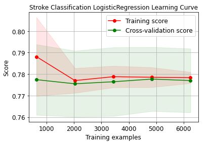
Let’s plot the LogisticRegression learning curve

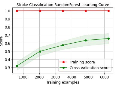
Let’s plot the RandomForest learning curve

skplt.estimators.plot_learning_curve(RandomForestClassifier(),train_x, train_y,
cv=7, shuffle=True, scoring=”r2″, n_jobs=-1,
figsize=(6,4), title_fontsize=”large”, text_fontsize=”large”,
title=”Stroke Classification RandomForest Learning Curve”);

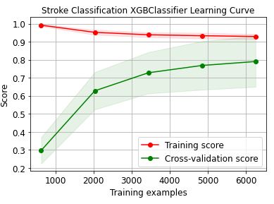
Let’s plot the XGBClassifier learning curve

skplt.estimators.plot_learning_curve(XGBClassifier(),train_x, train_y,
cv=7, shuffle=True, scoring=”r2″, n_jobs=-1,
figsize=(6,4), title_fontsize=”large”, text_fontsize=”large”,
title=”Stroke Classification XGBClassifier Learning Curve”);

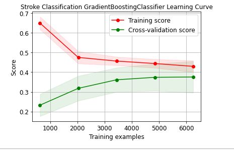
Let’s plot the GradientBoosting learning curve

skplt.estimators.plot_learning_curve(GradientBoostingClassifier(),train_x, train_y,
cv=7, shuffle=True, scoring=”r2″, n_jobs=-1,
figsize=(6,4), title_fontsize=”large”, text_fontsize=”large”,
title=”Stroke Classification GradientBoostingClassifier Learning Curve”);

Let’s plot the ExtraTrees learning curve

skplt.estimators.plot_learning_curve(ExtraTreesClassifier(),train_x, train_y,
cv=7, shuffle=True, scoring=”r2″, n_jobs=-1,
figsize=(6,4), title_fontsize=”large”, text_fontsize=”large”,
title=”Stroke Classification ExtraTreesClassifier Learning Curve”);

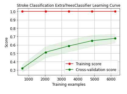
These learning curves confirm that the XGBClassifier is the best performer in terms of the training/X-validation scores and confidence intervals.

TF Performance Analysis

Let’s continue the GradientBoostingClassifier prediction QC analysis by invoking the TensorFlow library.

!pip install tensorflow

import tensorflow as tf
from tensorflow.keras.wrappers.scikit_learn import KerasClassifier
from sklearn.model_selection import cross_val_score

Y_test_probs = xgc.predict_proba(test_x)

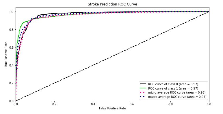
skplt.metrics.plot_roc_curve(test_y, Y_test_probs,
title=”Stroke Prediction ROC Curve”, figsize=(12,6));

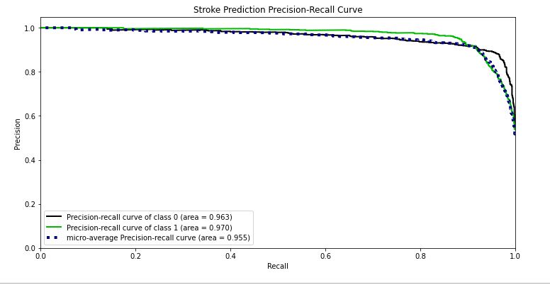
skplt.metrics.plot_precision_recall_curve(test_y, Y_test_probs,
title=”Stroke Prediction Precision-Recall Curve”, figsize=(12,6));

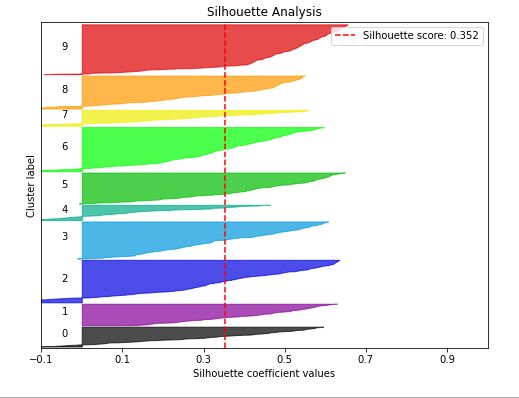
kmeans = KMeans(n_clusters=10, random_state=1)
kmeans.fit(train_x, train_y)
cluster_labels = kmeans.predict(test_x)

skplt.metrics.plot_silhouette(test_x, cluster_labels,
figsize=(8,6));

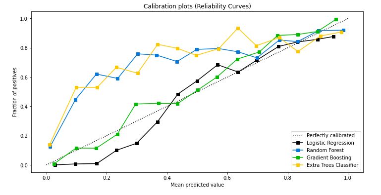
lr_probas = LogisticRegression().fit(train_x, train_y).predict_proba(test_x)
rf_probas = RandomForestClassifier().fit(train_x, train_y).predict_proba(test_x)
gb_probas = GradientBoostingClassifier().fit(train_x, train_y).predict_proba(test_x)
et_scores = ExtraTreesClassifier().fit(train_x, train_y).predict_proba(test_x)

probas_list = [lr_probas, rf_probas, gb_probas, et_scores]
clf_names = [‘Logistic Regression’, ‘Random Forest’, ‘Gradient Boosting’, ‘Extra Trees Classifier’]

skplt.metrics.plot_calibration_curve(test_y,
probas_list,
clf_names, n_bins=15,
figsize=(12,6)
);

rf = GradientBoostingClassifier()
rf.fit(train_x, train_y)

Y_cancer_probas = rf.predict_proba(test_x)

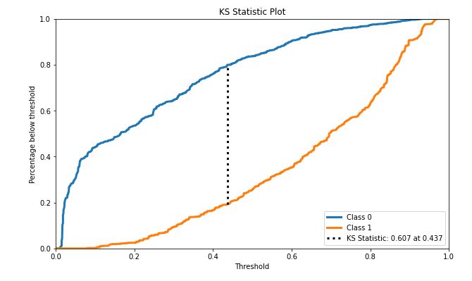
skplt.metrics.plot_ks_statistic(test_y, Y_cancer_probas, figsize=(10,6));

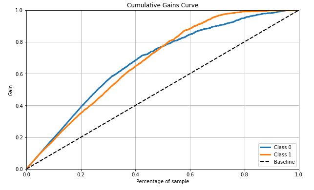
skplt.metrics.plot_cumulative_gain(test_y, Y_cancer_probas, figsize=(10,6));

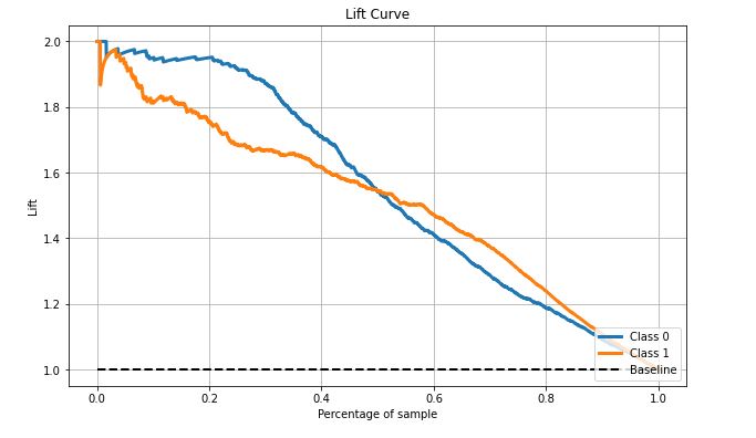
skplt.metrics.plot_lift_curve(test_y, Y_cancer_probas, figsize=(10,6));

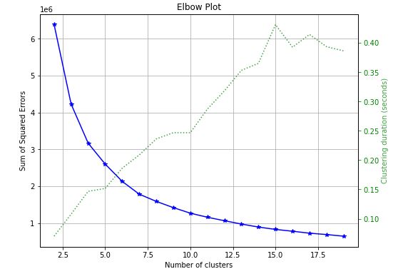
skplt.cluster.plot_elbow_curve(KMeans(random_state=1),
train_x,
cluster_ranges=range(2, 20),
figsize=(8,6));

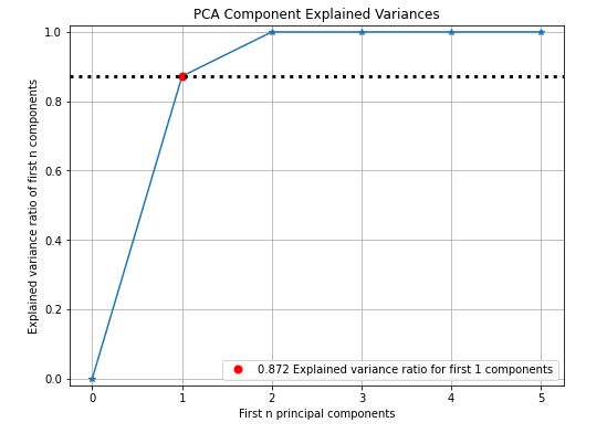
pca = PCA(random_state=1)
pca.fit(train_x)

skplt.decomposition.plot_pca_component_variance(pca, figsize=(8,6));

skplt.decomposition.plot_pca_2d_projection(pca, train_x, train_y,
figsize=(10,10),
cmap=”tab10″);

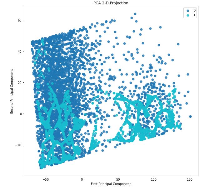
We can see the data is non-linear and also some interesting clustering. This suggests a high-dimension classification model or clustering model will work nicely.

Binary Classification Summary Report

Let’s summarize our best prediction classification results

Accuracy -->  0.9117889530090684
F1 Score -->  0.9066317626527051
Classification Report  --> 
               precision    recall  f1-score   support

           0       0.97      0.87      0.92      1347
           1       0.86      0.96      0.91      1079

    accuracy                           0.91      2426
   macro avg       0.91      0.92      0.91      2426
weighted avg       0.92      0.91      0.91      2426

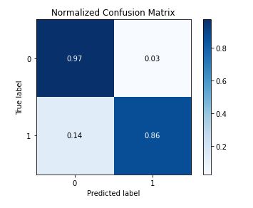
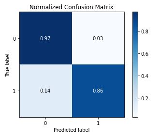
skplt.metrics.plot_confusion_matrix(test_y, predict, normalize=True)

gc=GradientBoostingClassifier(n_estimators=100000,max_depth=5,learning_rate=0.001)
gc.fit(train_x,train_y)

GradientBoostingClassifier(learning_rate=0.001, max_depth=5,
                           n_estimators=100000)

predict=xgc.predict(test_x)
print(‘Accuracy –> ‘,accuracy_score(predict,test_y))
print(‘F1 Score –> ‘,f1_score(predict,test_y))
print(‘Classification Report –> \n’,classification_report(predict,test_y))

Accuracy -->  0.9117889530090684
F1 Score -->  0.9066317626527051
Classification Report  --> 
               precision    recall  f1-score   support

           0       0.97      0.87      0.92      1347
           1       0.86      0.96      0.91      1079

    accuracy                           0.91      2426
   macro avg       0.91      0.92      0.91      2426
weighted avg       0.92      0.91      0.91      2426

Conclusions

In this study, the best trained GradientBoosting Classifier on the SMOTE-balanced stroke dataset can predict a patient stroke with accuracy=91%, precision = 97%, recall = 96% and f1-score=90%. The summary outcome of our performance QC analysis is as follows:

learning curves
- average score ~0.4 +/- 0.08 and 0.02 for validation and training data, respectively
ROC curve area = 0.97
Precision-recall curve area = 0.963, 0.97 of class 0, 1
Silhouette score = 0.352
Calibration plot confirms that the GradientBoosting is the best Classifier
KS statistic 0.607 at 0.437
Cumulate gains curve is max 60% deviates from baseline at 50% samples
Lift is ~ 1.55 at 50% samples
Elbow plot – the optimal number of clusters is 6
PCA analysis – 0.872 explained variance ratio for first 1 components
PCA 2-D projection – we can see the data is non-linear and also some interesting clustering. This suggests a high-dimension classification model or clustering model will work nicely.

References

[1] https://www.researchgate.net/publication/352261064

[2] https://doi.org/10.1016/j.health.2022.100032

[3] https://doi.org/10.1016/j.jstrokecerebrovasdis.2020.105162

[4] https://orfe.princeton.edu/

38 responses to “AI-Powered Stroke Prediction”

Hairstyles says:

21st Oct 2022 at 9:09 am

Hi, I think your blog might be having browser compatibility issues. When I look at your blog in Chrome, it looks fine but when opening in Internet Explorer, it has some overlapping. I just wanted to give you a quick heads up! Other then that, awesome blog!

LikeLiked by 1 person

- alxzp says:
  
  21st Oct 2022 at 9:49 am
  
  Thanks for your comment! Yes, Chrome is the default browser. Indeed, Google Chrome leads the web browser market with a 63.63% share, according to Statcounter. Apple Safari follows with 19.37%, Mozilla Firefox at 3.65%, Microsoft Edge (Chromium) at 3.24%, and Opera at 2.16%. Internet Explorer is still in use with 0.81%, while Microsoft Edge “Legacy” is fading out at 0.32%.
  
  LikeLiked by 1 person
  
Beauty Fashion says:

21st Oct 2022 at 2:42 pm

I think that is among the such a lot vital information for me. And i’m happy reading your article. But want to statement on some normal issues, The site taste is wonderful, the articles is actually great : D. Excellent job, cheers

LikeLiked by 1 person

Beauty Fashion says:

21st Oct 2022 at 8:05 pm

Thank you for the good writeup. It in fact was a amusement account it. Look advanced to far added agreeable from you! By the way, how can we communicate?

LikeLiked by 1 person

- alxzp says:
  
  21st Oct 2022 at 8:21 pm
  
  That’s [Get in Touch] @ Home (top right above explore).
  
  LikeLiked by 1 person
  
Beauty Fashion says:

21st Oct 2022 at 9:44 pm

Thanks for the sensible critique. Me & my neighbor were just preparing to do some research on this. We got a grab a book from our local library but I think I learned more clear from this post. I am very glad to see such wonderful information being shared freely out there.

LikeLiked by 1 person

Beauty Fashion says:

24th Oct 2022 at 12:48 pm

Hey very nice blog!! Man .. Beautiful .. Amazing .. I will bookmark your blog and take the feeds also厈I am happy to find a lot of useful information here in the post, we need work out more strategies in this regard, thanks for sharing. . . . . .

LikeLiked by 1 person

Beauty Fashion says:

27th Oct 2022 at 11:10 am

excellent post, very informative. I wonder why the other specialists of this sector do not notice this. You should continue your writing. I am confident, you have a huge readers’ base already!

LikeLiked by 1 person

Hairstyles says:

31st Oct 2022 at 6:29 am

This design is spectacular! You definitely know how to keep a reader amused. Between your wit and your videos, I was almost moved to start my own blog (well, almost…HaHa!) Excellent job. I really loved what you had to say, and more than that, how you presented it. Too cool!

LikeLiked by 1 person

Hairstyles says:

1st Nov 2022 at 4:01 am

Well I really liked studying it. This tip procured by you is very effective for correct planning.

LikeLiked by 1 person

Beauty Fashion says:

4th Nov 2022 at 11:32 am

I’ve observed that in the world today, video games include the latest fad with kids of all ages. Often times it may be out of the question to drag your son or daughter away from the activities. If you want the very best of both worlds, there are numerous educational activities for kids. Thanks for your post.

LikeLiked by 1 person

Fashion Styles says:

7th Nov 2022 at 8:03 pm

I would like to voice my appreciation for your kind-heartedness in support of all those that must have guidance on the concept. Your real commitment to getting the message around appeared to be surprisingly functional and has usually made workers like me to reach their aims. This valuable useful information denotes this much a person like me and far more to my peers. Regards; from all of us.

LikeLiked by 1 person

Beauty Fashion says:

9th Nov 2022 at 11:23 am

Good ?I should definitely pronounce, impressed with your web site. I had no trouble navigating through all tabs as well as related info ended up being truly easy to do to access. I recently found what I hoped for before you know it in the least. Reasonably unusual. Is likely to appreciate it for those who add forums or anything, web site theme . a tones way for your customer to communicate. Nice task..

LikeLiked by 1 person

Hairstyles says:

9th Nov 2022 at 6:15 pm

Usually I don’t learn article on blogs, but I would like to say that this write-up very compelled me to check out and do so! Your writing taste has been amazed me. Thanks, quite nice post.

LikeLiked by 1 person

Gal Jerman says:

11th Nov 2022 at 10:19 am

Top site ,.. amazaing post ! Just keep the work on !

LikeLiked by 1 person

Hairstyles says:

11th Nov 2022 at 11:18 am

Thanks for another fantastic article. Where else could anybody get that type of info in such an ideal way of writing? I’ve a presentation next week, and I’m on the look for such information.

LikeLiked by 1 person

Hairstyles says:

14th Nov 2022 at 11:56 am

Just wish to say your article is as amazing. The clearness to your submit is just spectacular and i can think you are a professional in this subject. Fine together with your permission allow me to seize your RSS feed to keep up to date with imminent post. Thank you 1,000,000 and please continue the gratifying work.

LikeLiked by 1 person

Hairstyles says:

14th Nov 2022 at 2:51 pm

Wow! Thank you! I permanently wanted to write on my site something like that. Can I include a part of your post to my blog?

LikeLiked by 1 person

Beauty Fashion says:

16th Nov 2022 at 10:52 am

I’ve been surfing on-line greater than 3 hours these days, but I by no means discovered any attention-grabbing article like yours. It抯 pretty price sufficient for me. Personally, if all website owners and bloggers made just right content material as you probably did, the web can be a lot more useful than ever before.

LikeLiked by 1 person

Hairstyles says:

16th Nov 2022 at 10:59 am

Very efficiently written post. It will be useful to everyone who usess it, including myself. Keep doing what you are doing – can’r wait to read more posts.

LikeLiked by 1 person

Hairstyles says:

16th Nov 2022 at 2:26 pm

Lovely site! I am loving it!! Will come back again. I am bookmarking your feeds also.

LikeLiked by 1 person

Hairstyles says:

19th Nov 2022 at 2:01 am

Wonderful beat ! I would like to apprentice at the same time as you amend your site, how can i subscribe for a blog website? The account aided me a acceptable deal. I have been a little bit acquainted of this your broadcast provided shiny clear idea

LikeLiked by 1 person

Hairstyles says:

19th Nov 2022 at 2:47 am

Good post. I be taught something more challenging on totally different blogs everyday. It’s going to at all times be stimulating to read content material from different writers and observe slightly one thing from their store. I抎 favor to make use of some with the content on my weblog whether you don抰 mind. Natually I抣l give you a hyperlink in your internet blog. Thanks for sharing.

LikeLiked by 1 person

Beauty Fashion says:

3rd Dec 2022 at 5:26 am

A formidable share, I just given this onto a colleague who was doing a little analysis on this. And he in truth bought me breakfast because I discovered it for him.. smile. So let me reword that: Thnx for the deal with! However yeah Thnkx for spending the time to discuss this, I feel strongly about it and love reading extra on this topic. If possible, as you turn into experience, would you thoughts updating your weblog with more details? It is highly helpful for me. Massive thumb up for this blog post!

LikeLiked by 1 person

Hairstyles says:

9th Dec 2022 at 12:05 pm

Magnificent beat ! I would like to apprentice while you amend your site, how can i subscribe for a blog website? The account helped me a appropriate deal. I were a little bit acquainted of this your broadcast offered brilliant transparent idea

LikeLiked by 1 person

- alxzp says:
  
  9th Dec 2022 at 1:47 pm
  
  Hi, thanks for your feedback! Sure, you can always subscribe for the website by entering your email address within the “Subscribe” input field at the bottom of the blog.
  
  LikeLike
  
Hairstyles says:

9th Dec 2022 at 12:14 pm

I have observed that in the world nowadays, video games will be the latest trend with children of all ages. Periodically it may be out of the question to drag your children away from the video games. If you want the best of both worlds, there are numerous educational video games for kids. Good post.

LikeLiked by 1 person

- alxzp says:
  
  9th Dec 2022 at 1:23 pm
  
  Hi there! Thanks for your feedback! In addition to video games, our fully automated end-to-end solutions can engage kids of all ages in learning. Indeed, we work hard to provide quality learning opportunities that prepare children with the knowledge and skill.
  Stay connected!
  
  LikeLike
  
Hairstyles says:

11th Dec 2022 at 2:00 am

This is really interesting, You are a very skilled blogger. I have joined your rss feed and look forward to seeking more of your magnificent post. Also, I have shared your site in my social networks!

LikeLiked by 1 person

Hairstyles says:

13th Dec 2022 at 12:11 am

This actually answered my drawback, thanks!

LikeLiked by 1 person

Beauty Fashion says:

13th Dec 2022 at 10:58 pm

I have recently started a web site, the information you provide on this site has helped me tremendously. Thank you for all of your time & work.

LikeLiked by 1 person

Faith Cooney says:

31st Dec 2022 at 4:42 am

A motivating dialogue is unquestionably worth comment. I feel that you need to produce far more on this topic, it will not be a taboo subject matter but commonly people don’t talk about these subjects. To another! Several many thanks!!

LikeLike

primeshred says:

19th Jan 2023 at 12:58 pm

It?s laborious to find educated folks on this subject, but you sound like you understand what you?re talking about! Thanks

LikeLike

Hairstyles says:

5th Feb 2023 at 4:37 am

You helped me a lot with this post. I love the subject and I hope you continue to write excellent articles like this.

LikeLike

Hairstyles says:

9th Feb 2023 at 8:25 pm

Thank you for being of assistance to me. I really loved this article.

LikeLike

intermittent fasting schedule says:

19th Feb 2023 at 10:35 am

Excellent post. I was checking constantly this blog and I’m impressed! Very useful information particularly the last part 🙂 I care for such information a lot. I was looking for this particular information for a very long time. Thank you and good luck.

LikeLike

Argentina SEO Backlink says:

19th Feb 2023 at 4:28 pm

I’ve been surfing online greater than three hours these days, yet I never found any attention-grabbing article like yours. It is lovely value sufficient for me. In my opinion, if all website owners and bloggers made excellent content material as you did, the net shall be much more useful than ever before.

LikeLike

Dumbbell Workout says:

24th Feb 2023 at 12:52 am

I just like the helpful info you supply to your articles. I?ll bookmark your blog and check again right here frequently. I am moderately certain I will be told many new stuff proper here! Good luck for the following!

LikeLike