
- This work aims to solve the problem of Markowitz portfolio optimization for a one-year horizon investment, through the pairs trading cointegrated strategy.
- Specifically, we’ll look at market-neutral trading strategies (MNTS). The goal of MNTS is to generate returns that are independent of market swings and achieve a zero beta against its relevant market index.
- Market-neutral alpha strategy is an investment method designed to provide significant alpha but little or no beta. Here, beta refers to the correlation of an investment with the usual swings in a broad stock market index such as the S&P 500, while alpha refers to the excess return beyond the market return earned through active trading.
- Statistical arbitrage (SA) is a classical example of MNTS. SA involves exploiting the price discrepancies of financial instruments that are highly correlated.
- We’ll analyze the relationship between market efficiency and a SA technique based on portfolio efficient frontiers combined with popular technical indicators, the Z-score analysis, and portfolio backtesting in 2023.
- We’ll examine asset allocation across a number of sectors including technology, financial services, and industrials.
- To measure the return of the portfolio, this article uses the annualized return of the portfolio.
- In the sequel, our MNTS consists of the following steps: (1) evaluate our financial goals, time horizon, and resources to achieve your goals; (2) study the financial markets and investment tools, including stocks, bonds, and derivatives, to know the instruments to use for our strategy; (3) formulate our strategy (which could be statistical arbitrage, merger arbitrage, pair trading, or any other) and backtest it.
Table of Contents
- Credits
- Correlations with AAPL
- AAPL Stat-Arb Backtesting
- Portfolio Efficient Frontiers
- AAPL Technical Indicators
- Cointegrated Pairs of Stocks
- Z-Score vs Trading Signals
- Conclusions
- Explore More
Credits
- Naive Statistical Arbitrage Trading Analysis
- Analysis of a Naive Statistical Arbitrage for Trading
- Momentum and Reversion Trading Signals Analysis
- adamd1985
Correlations with AAPL
- Setting the working directory YOURPATH
import os
os.chdir('YOURPATH')    # Set working directory
os. getcwd()
- Copying the utility functions analysis_utils.py to YOURPATH
- Importing the key libraries and reading the input stock data
import numpy as np
import pandas as pd
import matplotlib.pyplot as plt
import seaborn as sns
import warnings
warnings.filterwarnings("ignore")

import yfinance as yf
from analysis_utils import calculate_profit, load_ticker_prices_ts_df, plot_strategy, load_ticker_ts_df
START_DATE = "2020-01-01"
END_DATE = "2023-12-24"
tickers = ["AAPL", "MSFT", "AMZN", "TSLA", "GOOG", "XOM", "META", "NVDA", "PEP", "AVGO", "ADBE", "COST", "PYPL", "AMD", "QCOM", "INTC", "TXN", "CHTR", "TMUS", "ISRG", "SBUX", "AMGN", "INTU", "ADP", "CSX", "ADI", "MU", "ZM", "MAR", "GILD", "MELI", "WDAY", "PG", "PANW", "REGN", "RCL", "BKNG", "JNJ", "ADSK", "KLAC", "BAC"]

tickers_df = load_ticker_prices_ts_df(tickers, START_DATE, END_DATE)
tickers_rets_df = tickers_df.dropna(axis=1).pct_change().dropna()  # first % is NaN

# 1+ to allow the cumulative product of returns over time, and -1 to remove it at the end.
tickers_rets_df = (1 + tickers_rets_df).cumprod() - 1

plt.figure(figsize=(11, 11))
for ticker in tickers_rets_df.columns:
    plt.plot(tickers_rets_df.index, tickers_rets_df[ticker] * 100.0, label=ticker)

plt.xlabel("Date (Year-Month)")
plt.ylabel("Cummulative Returns(%")
plt.legend()
plt.show()
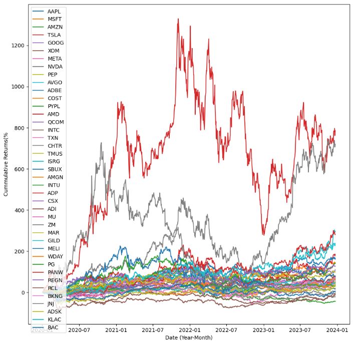
- Following the Macroaxis trading ideas, let’s examine the Apple stock correlation with its peers.
- Selecting peers with correlation > 0.75
TARGET = "AAPL"
MA_WINDOW = 24
ARB_WINDOW = MA_WINDOW * 10
plt.figure(figsize=(10, 6))

corr_ticks = []
LEADS = []

for ticker in tickers:
    if ticker == TARGET:
        continue
    correlation = tickers_df[ticker].corr(tickers_df[TARGET])
    if abs(correlation) < 0.75:
        continue

    LEADS.append(ticker)

    corr_ts = tickers_df[ticker].rolling(ARB_WINDOW).corr(tickers_df[TARGET])
    plt.plot(
        tickers_df.index,
        corr_ts.rolling(MA_WINDOW).mean(),
        label=f"{ticker} (Corr: {correlation:.2f})",
        alpha=correlation,
        linewidth=2,
    )
    corr_ticks.append(ticker)

plt.axhline(y=0, color="k", linestyle="--", linewidth=1)

plt.xlabel("Date (Year-Month)")
plt.ylabel("Correlation with AAPL")
plt.legend()
plt.show()
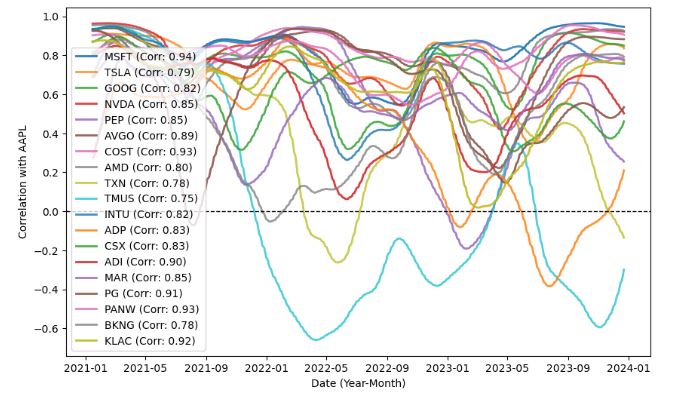
- It is clear that some stocks oscillate between uncorrelated and correlated in ’23.
- Calculating EMA and the covariance ratios between stock pairs
arb_df = tickers_rets_df.copy()
arb_df["price"] = tickers_df[TARGET]
arb_df[f"ema_{TARGET}"] = arb_df[TARGET].ewm(MA_WINDOW).mean()
arb_df[f"ema_d_{TARGET}"] = arb_df[TARGET] - arb_df[f"ema_{TARGET}"]
arb_df[f"ema_d_{TARGET}"].fillna(0, inplace=True)

for ticker in LEADS:
    arb_df[f"ema_{ticker}"] = arb_df[ticker].ewm(MA_WINDOW).mean()
    arb_df[f"ema_d_{ticker}"] = arb_df[ticker] - arb_df[f"ema_{ticker}"]
    arb_df[f"ema_d_{ticker}"].fillna(0, inplace=True)
    arb_df[f"{ticker}_corr"] = (
        arb_df[f"ema_d_{ticker}"].rolling(ARB_WINDOW).corr(arb_df[f"ema_d_{TARGET}"])
    )
    arb_df[f"{ticker}_covr"] = (
        arb_df[[f"ema_d_{ticker}", f"ema_d_{TARGET}"]]
        .rolling(ARB_WINDOW)
        .cov(numeric_only=True)
        .groupby(level=0, axis=0, dropna=True)  # Cov returns pairwise!
        .apply(lambda x: x.iloc[0, 1] / x.iloc[0, 0])
    )
    arb_df[f"{ticker}_emas_d_prj"] = (
        arb_df[f"ema_d_{ticker}"] * arb_df[f"{ticker}_covr"]
    )
    arb_df[f"{ticker}_emas_act"] = (
        arb_df[f"{ticker}_emas_d_prj"] - arb_df[f"ema_d_{TARGET}"]
    )

arb_df.filter(regex=f"(_emas_d_prj|_corr|_covr)$").dropna().iloc[ARB_WINDOW:]
- Calculating the AAPL_signal weights based on absolute values of correlations
ts = 0
delta_projected = 0
weights=0
for ticker in LEADS:
    corr_abs = abs(arb_df[f"{ticker}_corr"].fillna(0))
    weights += corr_abs
    arb_df[f"{ticker}_emas_act_w"] = arb_df[f"{ticker}_emas_act"].fillna(0) * corr_abs
    delta_projected += arb_df[f"{ticker}_emas_act_w"]

weights = weights.replace(0, 1)
arb_df[f"{TARGET}_signal"] = delta_projected / weights
arb_df[f"{TARGET}_signal"].iloc[ARB_WINDOW:]
- Calculating errors and the signals confidence intervals at 95%
errors = (
    arb_df[f"ema_{TARGET}"] + arb_df[f"ema_d_{TARGET}"] + arb_df[f"{TARGET}_signal"]
) - (arb_df[f"ema_{TARGET}"].shift(-1))
arb_df["rmse"] = np.sqrt((errors**2).rolling(ARB_WINDOW).mean()).fillna(0)

me = errors.rolling(ARB_WINDOW).mean().fillna(0)
e_std = errors.rolling(ARB_WINDOW).std().fillna(0)
ci = (me - 1.96 * e_std, me + 1.96 * e_std)
arb_df["ci_lower"] = arb_df[f"{TARGET}_signal"].fillna(0) + ci[0]
arb_df["ci_upper"] = arb_df[f"{TARGET}_signal"].fillna(0) + ci[1]
arb_df["ci_spread"] = arb_df["ci_upper"] - arb_df["ci_lower"]
arb_df.fillna(0, inplace=True)
arb_df[["ci_lower", "ci_upper"]].iloc[ARB_WINDOW:].tail(10)
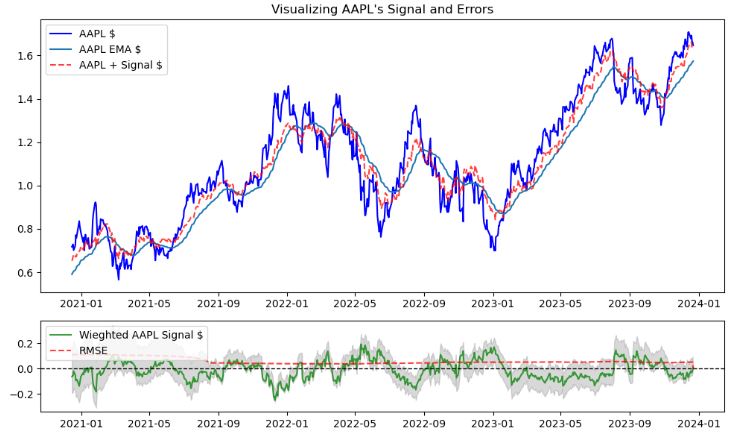
- Plotting the AAPL’s signal and errors
fig, axes = plt.subplots(2, 1, gridspec_kw={"height_ratios": (3, 1)}, figsize=(10, 6))

axes[0].set_title(f"Visualizing {TARGET}'s Signal and Errors")
axes[0].plot(
    arb_df.iloc[ARB_WINDOW:].index,
    arb_df[TARGET].iloc[ARB_WINDOW:],
    label=f"{TARGET} $",
    alpha=1,
    color="b",
)
axes[0].plot(
    arb_df.iloc[ARB_WINDOW:].index,
    arb_df[f"ema_{TARGET}"].iloc[ARB_WINDOW:],
    label=f"{TARGET} EMA $",
    alpha=1,
)
axes[0].plot(
    arb_df.iloc[ARB_WINDOW:].index,
    arb_df[f"{TARGET}_signal"].iloc[ARB_WINDOW:].fillna(0)
    + arb_df[TARGET].iloc[ARB_WINDOW:],
    label=f"{TARGET} + Signal $",
    alpha=0.75,
    linestyle="--",
    color="r",
)
axes[0].legend()
axes[1].plot(
    arb_df.iloc[ARB_WINDOW:].index,
    arb_df[f"{TARGET}_signal"].iloc[ARB_WINDOW:],
    label=f"Wieghted {TARGET} Signal $",
    alpha=0.75,
    color="g",
)
axes[1].plot(
    arb_df.iloc[ARB_WINDOW:].index,
    arb_df["rmse"].iloc[ARB_WINDOW:],
    label="RMSE",
    alpha=0.75,
    linestyle="--",
    color="r",
)
axes[1].fill_between(
    arb_df.iloc[ARB_WINDOW:].index,
    arb_df["ci_lower"].iloc[ARB_WINDOW:],
    arb_df["ci_upper"].iloc[ARB_WINDOW:],
    color="gray",
    alpha=0.3,
)
axes[1].axhline(0, color="black", linestyle="--", linewidth=1)
axes[1].legend()
plt.tight_layout()
plt.show()
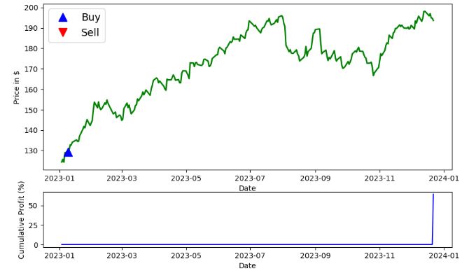
AAPL Stat-Arb Backtesting
- Let’s perform AAPL backtesting by acting upon the above trading signals with the following simulation parameters
LONG_THRESHOLD = 0.0025
SHORT_THRESHOLD = -0.0025
CONF_SPREAD_THRESHOLD = 0.15
MAX_SHARES = 1
arb_df["orders"] = 0
signals = arb_df[f"{TARGET}_signal"]
prev_signals = signals.shift(-1)

add_long_cond = (signals > LONG_THRESHOLD) & (prev_signals <= LONG_THRESHOLD) & (signals < arb_df["ci_upper"]) & (signals > arb_df["ci_lower"]) & (arb_df["ci_spread"] < CONF_SPREAD_THRESHOLD)
add_short_cond = (signals < SHORT_THRESHOLD) & (prev_signals >= SHORT_THRESHOLD) & (signals < arb_df["ci_upper"]) & (signals > arb_df["ci_lower"]) & (arb_df["ci_spread"] < CONF_SPREAD_THRESHOLD)


arb_df.loc[add_long_cond, "orders"] += MAX_SHARES
arb_df.loc[add_short_cond, "orders"] -= MAX_SHARES

arb_df["orders"].fillna(0, inplace=True)
arb_df.loc[arb_df["orders"] != 0, "orders"].tail(10)

2022-03-18 00:00:00    1
2022-04-08 00:00:00   -1
2022-04-12 00:00:00    1
2022-04-13 00:00:00   -1
2022-05-03 00:00:00    1
2022-05-04 00:00:00   -1
2023-11-01 00:00:00    1
2023-11-02 00:00:00   -1
2023-11-03 00:00:00    1
2023-12-21 00:00:00   -1
Name: orders, dtype: int64

signal_changes_df = arb_df.loc[(add_long_cond | add_short_cond), ["price", "orders", f"{TARGET}_signal"]]

signal_changes_df["holdings"] = signal_changes_df["orders"].cumsum()
signal_changes_df["stat_chng"] = np.sign(signal_changes_df["orders"].shift(1)) != np.sign(signal_changes_df["orders"])
prev_holdings = signal_changes_df["holdings"].shift(1)

signal_changes_df["price_open"] = signal_changes_df["price"].shift(1)
signal_changes_df["cost_open_avg"] = (signal_changes_df.loc[signal_changes_df["stat_chng"] == False, "price_open"].shift(1) + signal_changes_df.loc[signal_changes_df["stat_chng"]== False, "price_open"]) / 2
signal_changes_df["cost_open_avg"].fillna(signal_changes_df["price_open"], inplace=True)
signal_changes_df["price_close"] = signal_changes_df["price"]
signal_changes_df["price_close"].iloc[0] = np.nan  # First signal shouldn't have a closing price

signal_changes_df["pnl"] = (signal_changes_df.loc[signal_changes_df["stat_chng"], "price_close"]  - signal_changes_df.loc[signal_changes_df["stat_chng"], "cost_open_avg"]) * np.sign(signal_changes_df["holdings"].shift(1))
signal_changes_df["pnl_rets"] = signal_changes_df["pnl"] / signal_changes_df["cost_open_avg"].abs()
signal_changes_df.fillna(0, inplace=True)

arb_df = pd.concat([arb_df, signal_changes_df[["pnl", "pnl_rets", "holdings"]]], axis=1).drop_duplicates(keep='last')

#signal_changes_df.tail(10)
- Plotting the AAPL simulated trades and cumulative returns
plt.figure(figsize=(12, 7))

fig, (ax1, ax2, ax3) = plt.subplots(
    3, 1, gridspec_kw={"height_ratios": (3, 1, 1)}, figsize=(12, 7)
)

ax1.plot(
    arb_df.iloc[ARB_WINDOW:].index,
    arb_df["price"].iloc[ARB_WINDOW:],
    color="g",
    lw=1.25,
    label=f"{TARGET}",
)
ax1.plot(
    arb_df.loc[add_long_cond].index,
    arb_df.loc[add_long_cond, "price"],
    "^",
    markersize=12,
    color="blue",
    label="Buy",
)
ax1.plot(
    arb_df.loc[add_short_cond].index,
    arb_df.loc[add_short_cond, "price"],
    "v",
    markersize=12,
    color="red",
    label="Sell",
)
ax1.set_ylabel("Price in $")
ax1.legend(loc="upper left", fontsize=14)
ax1.set_title(f"Stat-Arb {TARGET}", fontsize=18)

ax2.plot(
    arb_df["pnl"].iloc[ARB_WINDOW:].index, arb_df["pnl_rets"].iloc[ARB_WINDOW:].fillna(0).cumsum(), color="b", label="Returns"
)
ax2.set_ylabel("Cumulative Profit (%)")
ax2.legend(loc="upper left", fontsize=10)
ax2.set_title(f"Cumulative Returns", fontsize=18)

ax3.plot(
    arb_df.iloc[ARB_WINDOW:].index,
    arb_df[f"{TARGET}_signal"].iloc[ARB_WINDOW:],
    label=f"Signal",
    alpha=0.75,
    color="g",
)
ax3.plot(
    arb_df.loc[add_long_cond].index,
    arb_df.loc[add_long_cond, f"{TARGET}_signal"],
    "^",
    markersize=12,
    color="blue",
    label="Buy",
)
ax3.plot(
    arb_df.loc[add_short_cond].index,
    arb_df.loc[add_short_cond, f"{TARGET}_signal"],
    "v",
    markersize=12,
    color="red",
    label="Sell",
)
ax3.axhline(0, color="black", linestyle="--", linewidth=1)
ax3.axhline(SHORT_THRESHOLD, color="r", linestyle="--", label=f"Short ({SHORT_THRESHOLD})",linewidth=1)
ax3.axhline(LONG_THRESHOLD, color="b", linestyle="--", label=f"Long ({LONG_THRESHOLD})",linewidth=1)
ax3.fill_between(arb_df.index, arb_df[f"{TARGET}_signal"], SHORT_THRESHOLD, where=(arb_df[f"{TARGET}_signal"] < SHORT_THRESHOLD), interpolate=True, color='red', alpha=0.3)
ax3.fill_between(arb_df.index, arb_df[f"{TARGET}_signal"], LONG_THRESHOLD, where=(arb_df[f"{TARGET}_signal"] > LONG_THRESHOLD), interpolate=True, color='blue', alpha=0.3)
ax3.fill_between(
    arb_df.iloc[ARB_WINDOW:].index,
    arb_df["ci_lower"].iloc[ARB_WINDOW:],
    arb_df["ci_upper"].iloc[ARB_WINDOW:],
    color="gray",
    alpha=0.3,
    label=f"Confidence"
)
ax3.legend(loc="lower left", fontsize=12)
ax3.set_title(f"Leads' Signal", fontsize=18)

plt.tight_layout()
plt.show()
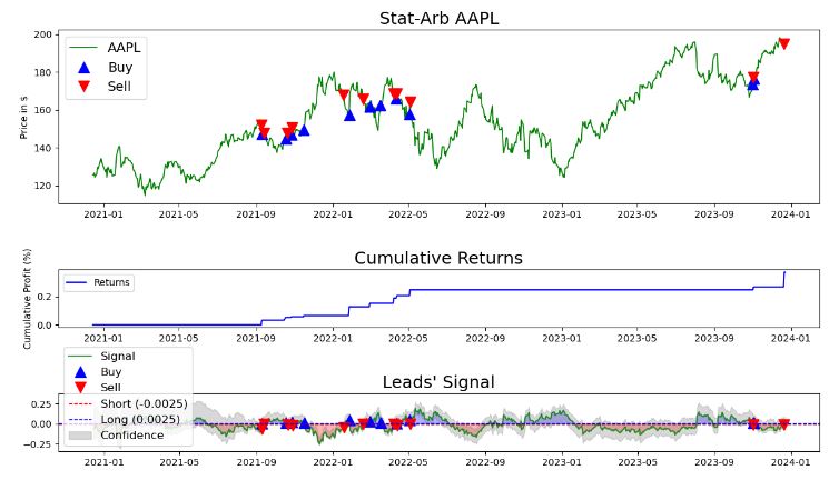
- It appears that simulated trading yields the cumulative return return of 40%.
Portfolio Efficient Frontiers
- Let’s discuss the Efficient Frontier, a core concept in Harry Markowitz’s Modern Portfolio Theory (MPT). MPT is used in quantitative finance to build optimal portfolios that offer the highest expected return for a given level of risk.
- Importing the key libraries and selecting the portfolio of interest
import numpy as np
import pandas as pd
import matplotlib.pyplot as plt
import yfinance as yf
from analysis_utils import calculate_profit, load_ticker_prices_ts_df, plot_strategy, load_ticker_ts_df
tickers = ["META", "AAPL","NVDA","TSLA","BAC","JNJ"]

START_DATE = "2020-01-01"
END_DATE = "2022-12-31"

tickers_orig_df = load_ticker_prices_ts_df(tickers, START_DATE, END_DATE)
tickers_df = tickers_orig_df.dropna(axis=1).pct_change().dropna()  # first % is NaN

# 1+ to allow the cumulative product of returns over time, and -1 to remove it at the end.
tickers_df = (1 + tickers_df).cumprod() - 1

plt.figure(figsize=(10, 6))
for ticker in tickers_df.columns:
    plt.plot(tickers_df.index, tickers_df[ticker] * 100.0, label=ticker)

plt.xlabel("Date (Year-Month)")
plt.ylabel("Cumulative Returns(%)")
plt.legend()
plt.show()
![Cumulative Returns(%) of selected stocks: tickers = ["META", "AAPL","NVDA","TSLA","BAC","JNJ"]](https://newdigitals.org/wp-content/uploads/2023/12/eff_portfolio-1.jpg?w=653)
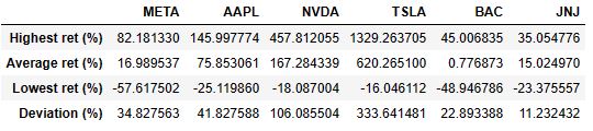
- Calculating the following descriptive statistics of cumulative returns
mean_returns = tickers_df.mean()
highest_returns = tickers_df.max()
lowest_returns = tickers_df.min()
std_deviation = tickers_df.std()
summary_table = pd.DataFrame(
    {
        "Highest ret (%)": highest_returns * 100.0,
        "Average ret (%)": mean_returns * 100.0,
        "Lowest ret (%)": lowest_returns * 100.0,
        "Deviation (%)": std_deviation * 100.0,
    }
)
summary_table.transpose()
- Experimenting with the investors choices of risk/reward, through indifference curves.
def utility_fn(x, a=0.15, b=0.1, c=1):
    return a * x**2 + b * x + c


plt.figure(figsize=(10, 6))

x_values_1 = np.linspace(0, 40, 100)
y_values_1 = utility_fn(x_values_1, c=10)
plt.plot(x_values_1, y_values_1, label="Low Utility", alpha=0.6)

x_values_2 = np.linspace(0, 35, 100)
y_values_2 = utility_fn(x_values_2, c=24)
plt.plot(x_values_2, y_values_2, label="Moderate Utility", color="g", alpha=0.6)

x_values_3 = np.linspace(0, 30, 100)
y_values_3 = utility_fn(x_values_3, c=35)
plt.plot(x_values_3, y_values_3, label="High Utility", color="r", alpha=0.6)

plt.plot([0, 40], [5, 140], label="Opportunity Set", color="b", linewidth=2)

plt.plot([2, 2], [0, 12], linestyle="--", color="b", alpha=0.6, linewidth=2)
plt.plot([0, 2], [12, 12], linestyle="--", color="b", alpha=0.6, linewidth=2)
plt.plot([10, 10], [0, 40], linestyle="--", color="g", alpha=0.6, linewidth=2)
plt.plot([0, 10], [40, 40], linestyle="--", color="g", alpha=0.6, linewidth=2)
plt.plot([20, 20], [0, 72], linestyle="--", color="b", alpha=0.6, linewidth=2)
plt.plot([0, 20], [72, 72], linestyle="--", color="b", alpha=0.6, linewidth=2)

plt.xlabel("Risk %")
plt.ylabel("Returns %")
plt.title("Utility Curves (Risk Free VS AAPL)")
plt.legend()
plt.grid()

plt.xlim(0, 25)
plt.ylim(0, 100)
plt.show()
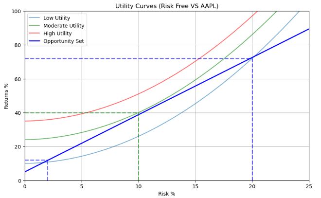
- The optimal choice is when the opportunity set line is tangent to a curve, in our case the
moderateutility curve, giving us 70% returns for 20% risk. - Computing the annual covariance matrix and returns of our stocks
TRADING_DAYS_IN_YEAR = 252

tickers_df = tickers_orig_df.dropna(axis=1).pct_change().dropna()

rets = ((1 + tickers_df).prod() ** (TRADING_DAYS_IN_YEAR / len(tickers_df))) - 1
cov_matrix = tickers_df.cov() * TRADING_DAYS_IN_YEAR
print(cov_matrix)

         META      AAPL      NVDA      TSLA       BAC       JNJ
META  0.237390  0.113085  0.164167  0.130005  0.074333  0.030630
AAPL  0.113085  0.136407  0.147414  0.138480  0.073008  0.038126
NVDA  0.164167  0.147414  0.313340  0.221768  0.093156  0.037974
TSLA  0.130005  0.138480  0.221768  0.521113  0.085079  0.021494
BAC   0.074333  0.073008  0.093156  0.085079  0.171712  0.042495
JNJ   0.030630  0.038126  0.037974  0.021494  0.042495  0.047665

print(round(rets*100,2))

META   -16.93
AAPL    20.91
NVDA    34.77
TSLA    62.65
BAC     -0.16
JNJ      9.37
dtype: float64
- A portfolio is a weighted collection of assets. Let’s create portfolios with randomly selected weights below
RISK_FREE_RATE = 0.05
MAX_PORTS = 10000
MAX_WEIGHT = 1.05


def port_generator(rets, cov_matrix):
    port_rets = []
    port_risks = []
    port_sharpes = []
    port_weights = []

    for _ in range(MAX_PORTS):
        # weights = np.random.random(len(rets))
        weights = np.random.uniform(-MAX_WEIGHT, MAX_WEIGHT, len(rets))
        weights /= np.sum(weights)  # Normalize weights to 1
        if any(weights > MAX_WEIGHT):
            continue
        port_weights.append(weights)

        port_ret = np.dot(weights, rets)
        port_rets.append(port_ret)

        port_risk = np.sqrt(weights.T @ cov_matrix @ weights)
        port_risks.append(port_risk)

        port_sharpe = (port_ret - RISK_FREE_RATE) / port_risk
        port_sharpes.append(port_sharpe)

    port_rets = np.array(port_rets)
    port_risks = np.array(port_risks)

    plt.scatter(
        port_risks * 100.0,
        port_rets * 100.0,
        c=port_sharpes,
        cmap="viridis",
        alpha=0.75,
    )

    plt.xlabel("Risk (%)")
    plt.ylabel("Expected Returns (%)")
    plt.colorbar(label="Sharpe Ratio")
    plt.grid()

    return port_risks, port_rets, port_sharpes


plt.figure(figsize=(10, 6))
plt.title("Random Portfolios")
port_risks, port_rets, port_sharpes=port_generator(rets, cov_matrix)
plt.show()
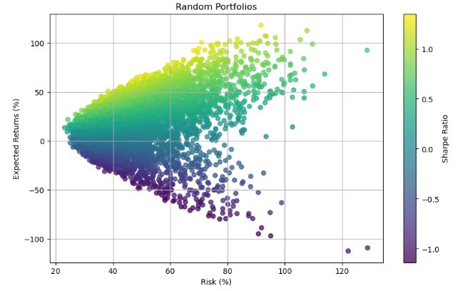
- Checking the portfolio risks
print(port_risks)
[0.33830614 0.31844794 0.515034   ... 0.62395826 0.51434099 0.41154064]
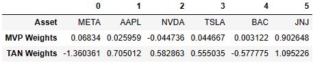
- Comparing minimum variance vs tangency portfolios
# Equal-weighted portfolio useful for matrix operations
equal_weights = np.ones(len(rets))
rets = ((1 + tickers_df).prod() ** (TRADING_DAYS_IN_YEAR / len(tickers_df))) - 1
cov_matrix = tickers_df.cov() * TRADING_DAYS_IN_YEAR
# Min variance weights
inv_cov_matrix = np.linalg.pinv(cov_matrix)
min_risk_vect = equal_weights @ inv_cov_matrix
expect_ret_vect = inv_cov_matrix @ rets
# Minimum variance portfolio
# Weights are normalized to sum to 1, and risk to std deviation.
mvp_weights = min_risk_vect / np.sum(min_risk_vect)
mvp_ret = mvp_weights @ rets
mvp_risk = np.sqrt(mvp_weights.T @ cov_matrix @ mvp_weights)
# Tangency portfolio
tan_weights = expect_ret_vect / np.sum(expect_ret_vect)
tan_ret = tan_weights @ rets
tan_risk = np.sqrt(tan_weights.T @ cov_matrix @ tan_weights)
summary_data = {
"Asset": tickers,
"MVP Weights": mvp_weights,
"TAN Weights": tan_weights,
}
print(f"mvp_ret: {mvp_ret*100:0.02f}%, mvp_risk {mvp_risk*100:0.02f}%")
print(f"tan_ret: {tan_ret*100:0.02f}%, tan_risk {tan_risk*100:0.02f}%")
summary_df = pd.DataFrame(summary_data)
summary_df.T
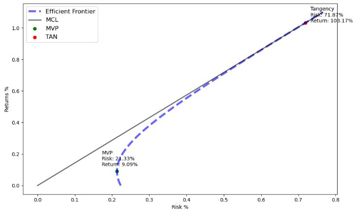
mvp_ret: 9.09%, mvp_risk 21.33%
tan_ret: 103.17%, tan_risk 71.87%
- Adding the Market Capital Line (MCL) to represent the market’s risk and returns at the time of this analysis, any portfolio under this line might be overpriced and suboptimal, any higher might be underpriced for its risk. When plotted against the expected returns, the CML will intercept the efficient frontier at the TAN portfolio, and this intercept is the most optimal market portfolio:
MAX_RETS = 1.1
TEN_BASIS_POINTS = 0.0001 * 10

c = np.sum(equal_weights * min_risk_vect)  # Constant term
b = np.sum(rets * min_risk_vect)  # Linear term
a = np.sum(rets * expect_ret_vect)  # Quadratic term
utility_func = (a * c) + (-(b**2))  # U(X) to penalize risk

# The frontier curve & MCL, scaled by utility function
exp_rets = np.arange(0, MAX_RETS, TEN_BASIS_POINTS)
ports_risk_frontier = np.sqrt(
    ((c * (exp_rets**2)) - (2 * b * exp_rets) + a) / utility_func
)
mcl_vector = exp_rets * (1 / np.sqrt(a))

plt.figure(figsize=(10, 6))
plt.plot(
    ports_risk_frontier,
    exp_rets,
    linestyle="--",
    color="blue",
    label="Efficient Frontier",
    linewidth=4,
    alpha=0.6,
)
plt.plot(
    mcl_vector,
    exp_rets,
    label="MCL",
    linewidth=2,
    alpha=0.6,
    color="black",
)

plt.scatter(mvp_risk, mvp_ret, color="green", label="MVP")
plt.annotate(
    f"MVP\nRisk: {mvp_risk*100:.2f}%\nReturn: {mvp_ret*100:.2f}%",
    (mvp_risk, mvp_ret),
    textcoords="offset points",
    xytext=(-30, 10),
)
plt.scatter(tan_risk, tan_ret, color="red", label="TAN")
plt.annotate(
    f"Tangency\nRisk: {tan_risk*100:.2f}%\nReturn: {tan_ret*100:.2f}%",
    (tan_risk, tan_ret),
    textcoords="offset points",
    xytext=(10, 1),
)

plt.legend(loc="upper left", fontsize=12)
plt.xlabel("Risk %")
plt.ylabel("Returns %")
plt.tight_layout()
plt.show()
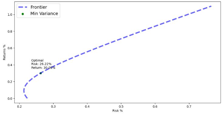
- Finding the min variance risk for the given return of 30%
TARGET_RET = 0.3

pt_port = None
opt_risk = None
opt_ret = None

mvp_weights = (a - (b * TARGET_RET)) / utility_func
tan_weights = ((c * TARGET_RET) - b) / utility_func

opt_port_weights = (mvp_weights * min_risk_vect) + (tan_weights * expect_ret_vect)
opt_ret = np.sum(opt_port_weights * rets)
opt_risk = np.sqrt(((c * (opt_ret**2)) - (2 * b * opt_ret) + a) / utility_func)

plt.figure(figsize=(12, 6))
plt.plot(
    ports_risk_frontier,
    exp_rets,
    linestyle="--",
    color="blue",
    label="Frontier",
    linewidth=4,
    alpha=0.6,
)

plt.scatter(opt_risk, opt_ret, color="green", label="Min Variance")
plt.annotate(
    f"Optimal \nRisk: {opt_risk*100:.2f}%\nReturn: {opt_ret*100:.2f}%",
    (opt_risk, opt_ret),
    textcoords="offset points",
    xytext=(-30, 15),
)

plt.legend(loc="upper left", fontsize=14)
plt.xlabel("Risk %")
plt.ylabel("Returns %")
plt.tight_layout
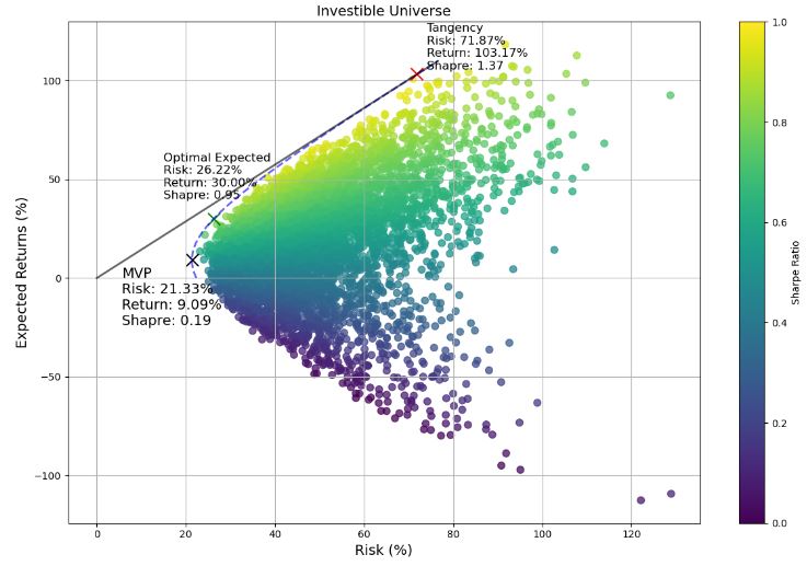
- Final output: the MVP, tangency points, the optimal expected risk, MCL, and the efficient frontier
# Add portfolios sharpe
opt_sharpe = (opt_ret - RISK_FREE_RATE) / opt_risk
mvp_sharpe = (mvp_ret - RISK_FREE_RATE) / mvp_risk
tan_sharpe = (tan_ret - RISK_FREE_RATE) / tan_risk

plt.figure(figsize=(12, 8))  # Increase figure size

plt.title("Investible Universe",fontsize=14)

plt.scatter(
    port_risks * 100.0,
    port_rets * 100.0,
    c=port_sharpes,
    cmap="viridis",
    alpha=0.75,
    s=50,  # Adjust the size of the scatter points
)

plt.plot(
    ports_risk_frontier * 100,
    exp_rets * 100,
    linestyle="--",
    color="blue",
    label="Frontier",
    linewidth=2,
    alpha=0.6,
)

# Adjust the size of the optimal point
plt.scatter(
    opt_risk * 100,
    opt_ret * 100,
    color="green",
    marker="x",
    s=150,
    label="Optimal Expected Returns",
)
plt.annotate(
    f"Optimal Expected \nRisk: {opt_risk*100:.2f}%\nReturn: {opt_ret*100:.2f}%\nShapre: {opt_sharpe:.2f}",
    (opt_risk * 100, opt_ret * 100),
    textcoords="offset points",
    xytext=(-50, 20),  # Adjust the annotation position
    fontsize=12,  # Adjust the font size
)

plt.plot(
    mcl_vector * 100,
    exp_rets * 100,
    label="MCL",
    linewidth=2,
    alpha=0.6,
    color="black",
)

# Adjust the size and position of the MVP point
plt.scatter(
    mvp_risk * 100,
    mvp_ret * 100,
    color="Black",
    label="MVP",
    marker="x",
    s=150,
)
plt.annotate(
    f"MVP\nRisk: {mvp_risk*100:.2f}%\nReturn: {mvp_ret*100:.2f}%\nShapre: {mvp_sharpe:.2f}",
    (mvp_risk * 100, mvp_ret * 100),
    textcoords="offset points",
    xytext=(-70, -65),
    fontsize=14,
)

# Adjust the size and position of the Tangency point
plt.scatter(
    tan_risk * 100,
    tan_ret * 100,
    color="red",
    label="TAN",
    marker="x",
    s=150,
)
plt.annotate(
    f"Tangency\nRisk: {tan_risk*100:.2f}%\nReturn: {tan_ret*100:.2f}%\nShapre: {tan_sharpe:.2f}",
    (tan_risk * 100, tan_ret * 100),
    textcoords="offset points",
    xytext=(10, 5),
    fontsize=12,
)

plt.xlabel("Risk (%)",fontsize=14)
plt.ylabel("Expected Returns (%)",fontsize=14)
plt.colorbar(label="Sharpe Ratio")
plt.grid()

plt.tight_layout()
plt.show()
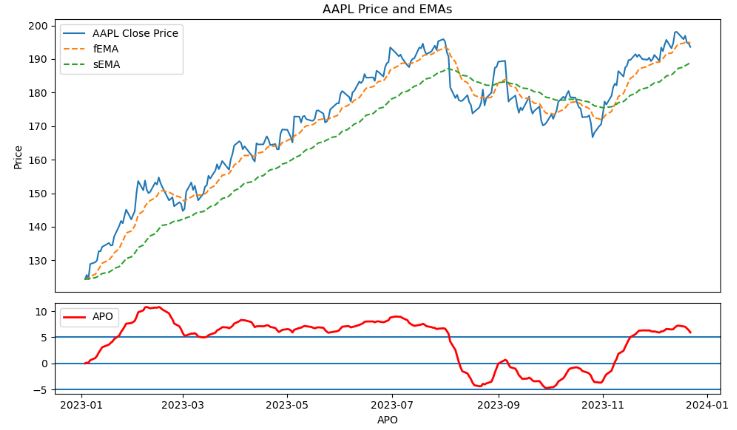
AAPL Technical Indicators
- Let’s compare the aforementioned findings to the results of technical analysis for AAPL in ’23.
- Consider the most popular trading strategies such as double SMA, naive momentum, mean reversion, APO, EMA, MACD, and RSI.
- Importing the key libraries
import numpy as np
import pandas as pd
import matplotlib.pyplot as plt

import yfinance as yf
from analysis_utils1 import calculate_profit, load_ticker_ts_df, plot_strategy
- Introducing the double SMA signals
APO_FAST_WINDOW=5
def double_simple_moving_average_signals(ticker_ts_df, short_window=5, long_window=30):
    """
    Generate trading signals based on a double simple moving average (SMA) strategy.
    Parameters:
    - aapl_ts_df (pandas.DataFrame): A DataFrame containing historical stock data.
    - short_window (int): The window size for the short-term SMA.
    - long_window (int): The window size for the long-term SMA.
    Returns:
    - signals (pandas.DataFrame): A DataFrame containing the trading signals.
    """
    signals = pd.DataFrame(index=ticker_ts_df.index)
    signals['signal'] = 0.0
    signals['short_mavg'] = ticker_ts_df['Close'].rolling(window=short_window,
                                                          min_periods=APO_FAST_WINDOW,
                                                          center=False).mean()
    signals['long_mavg'] = ticker_ts_df['Close'].rolling(window=long_window,
                                                         min_periods=APO_FAST_WINDOW,
                                                         center=False).mean()
    # Generate signal when SMAs cross
    signals['signal'] = np.where(
        signals['short_mavg'] > signals['long_mavg'], 1, 0)
    signals['orders'] = signals['signal'].diff()
    signals.loc[signals['orders'] == 0, 'orders'] = None
    return signals
- Plotting double SMA trading signals and cumulative returns for AAPL in ’23
aapl_ts_df = load_ticker_ts_df('AAPL',
                               start_date='2023-01-01',
                               end_date='2023-12-24')
signal_df = double_simple_moving_average_signals(aapl_ts_df, 5, 30)
profit_series = calculate_profit(signal_df, aapl_ts_df["Adj Close"])
ax1, ax2 = plot_strategy(aapl_ts_df["Adj Close"], signal_df, profit_series)

# Add short and long moving averages

ax1.plot(signal_df.index, signal_df['short_mavg'],
         linestyle='--', label='Fast SMA')
ax1.plot(signal_df.index, signal_df['long_mavg'],
         linestyle='--', label='Slow SMA')
ax1.legend(loc='upper left', fontsize=14)
plt.show()
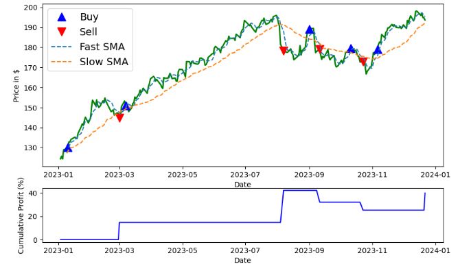
- It seems that the double SMA strategy yields the cumulative return of 40%.
- Generating naive momentum trading signals based on consecutive positive or negative price changes
def naive_momentum_signals(ticker_ts_df, nb_conseq_days=2):
    """
    Generate naive momentum trading signals based on consecutive positive or negative price changes.
    Parameters:
    - ticker_ts_df (pandas.DataFrame): A DataFrame containing historical stock data.
    - nb_conseq_days (int): The number of consecutive positive or negative days to trigger a signal.
    Returns:
    - signals (pandas.DataFrame): A DataFrame with 'orders' column containing buy (1) and sell (-1) signals.
    """
    signals = pd.DataFrame(index=ticker_ts_df.index)
    signals['orders'] = 0

    price = ticker_ts_df['Adj Close']
    price_diff = price.diff()

    signal = 0
    cons_day = 0

    for i in range(1, len(ticker_ts_df)):
        if price_diff[i] > 0:
            cons_day = cons_day + 1 if price_diff[i] > 0 else 0
            if cons_day == nb_conseq_days and signal != 1:
                signals['orders'].iloc[i] = 1
                signal = 1
        elif price_diff[i] < 0:
            cons_day = cons_day - 1 if price_diff[i] < 0 else 0
            if cons_day == -nb_conseq_days and signal != -1:
                signals['orders'].iloc[i] = -1
                signal = -1

    return signals


signal_df = naive_momentum_signals(aapl_ts_df)
profit_series = calculate_profit(signal_df, aapl_ts_df["Adj Close"])
ax1, _ = plot_strategy(aapl_ts_df["Adj Close"], signal_df, profit_series)

ax1.legend(loc='upper left', fontsize=14)
plt.show()
- It turns out that the naive momentum trading strategy yields the cumulative return over 60%.
- Generating mean reversion trading signals based on moving averages and thresholds
def mean_reversion_signals(ticker_ts_df, entry_threshold=1.0, exit_threshold=0.5):
    """
    Generate mean reversion trading signals based on moving averages and thresholds.
    Parameters:
    - ticker_ts_df (pandas.DataFrame): A DataFrame containing historical stock data.
    - entry_threshold (float): The entry threshold as a multiple of the standard deviation.
    - exit_threshold (float): The exit threshold as a multiple of the standard deviation.

    Returns:
    - signals (pandas.DataFrame): A DataFrame with 'orders' column containing buy (1) and sell (-1) signals.

    """
    signals = pd.DataFrame(index=ticker_ts_df.index)
    signals['mean'] = ticker_ts_df['Adj Close'].rolling(
        window=20).mean()  # Adjust the window size as needed
    signals['std'] = ticker_ts_df['Adj Close'].rolling(
        window=20).std()  # Adjust the window size as needed

    signals['signal'] = np.where(ticker_ts_df['Adj Close'] > (
        signals['mean'] + entry_threshold * signals['std']), 1, 0)
    signals['signal'] = np.where(ticker_ts_df['Adj Close'] < (
        signals['mean'] - exit_threshold * signals['std']), -1, 0)

    signals['orders'] = signals['signal'].diff()
    signals.loc[signals['orders'] == 0, 'orders'] = None

    return signals

signal_df = mean_reversion_signals(aapl_ts_df)
profit_series = calculate_profit(signal_df, aapl_ts_df["Adj Close"])
ax1, _ = plot_strategy(aapl_ts_df["Adj Close"], signal_df, profit_series)

ax1.plot(signal_df.index, signal_df['mean'], linestyle='--', label="Mean")
ax1.plot(signal_df.index, signal_df['mean'] +
         signal_df['std'], linestyle='--', label="Ceiling STD")
ax1.plot(signal_df.index, signal_df['mean'] -
         signal_df['std'], linestyle='--', label="Floor STD")
ax1.legend(loc='upper left', fontsize=10)
plt.show()

- It appears that the mean reversion trading strategy yields the cumulative return over 45%.
- Generating trading signals based on APO and double EMA for AAPL in ’23
import numpy as np
import pandas as pd
import matplotlib.pyplot as plt

import warnings
warnings.filterwarnings("ignore")

import yfinance as yf
from analysis_utils import calculate_profit, load_ticker_ts_df, plot_strategy

tickers = ['AAPL']

START_DATE = '2023-01-01'
END_DATE = '2023-12-24'
APO_BULL_SIGNAL = 5
APO_BEAR_SIGNAL = -5
APO_FAST_WINDOW = 12
APO_SLOW_WINDOW = 45

ticker = load_ticker_ts_df('AAPL', START_DATE, END_DATE)
ticker['fEMA'] = ticker['Adj Close'].ewm(
    span=APO_FAST_WINDOW, adjust=False).mean()
ticker['sEMA'] = ticker['Adj Close'].ewm(
    span=APO_SLOW_WINDOW, adjust=False).mean()
ticker['APO'] = ticker['fEMA'] - ticker['sEMA']

fig, (ax1, ax2) = plt.subplots(2, 1, gridspec_kw={
    'height_ratios': (3, 1)}, figsize=(10, 6))
ax1.plot(ticker.index, ticker['Adj Close'], label='AAPL Close Price')
ax1.plot(ticker.index, ticker['fEMA'], label='fEMA', linestyle='--')
ax1.plot(ticker.index, ticker['sEMA'], label='sEMA', linestyle='--')
ax1.set_title('AAPL Price and EMAs')
ax1.set_ylabel('Price')
ax1.set_xticks([])

ax2.axhline(APO_BULL_SIGNAL)
ax2.axhline(0.0)
ax2.axhline(APO_BEAR_SIGNAL)
ax2.plot(ticker.index, ticker['APO'], label='APO', lw=2, color='r')
ax2.set_xlabel('APO')

ax1.legend()
ax2.legend()
plt.tight_layout()
plt.show()
- Plotting the APO trading signals and cumulative returns for AAPL in ’23
def signal_apo_oscillator(ticker_ts, fast_window_size=APO_FAST_WINDOW, slow_window_size=APO_SLOW_WINDOW, buy_threshold=APO_BULL_SIGNAL, sell_threshold=APO_BEAR_SIGNAL):
    """
    Calculate signals using the Absolute Price Oscillator (APO) indicator for a given stock's time series.
    Parameters:
    - ticker_ts (DataFrame): Time series data for the stock, typically containing 'Adj Close' prices.
    - fast_window_size (int, optional): Fast EMA (Exponential Moving Average) window size. Default is APO_FAST_WINDOW.
    - slow_window_size (int, optional): Slow EMA window size. Default is APO_SLOW_WINDOW.
    - buy_threshold (float, optional): Buy signal threshold for the APO. Default is APO_BULL_SIGNAL.
    - sell_threshold (float, optional): Sell signal threshold for the APO. Default is APO_BEAR_SIGNAL.
    Returns:
    - signals_df (DataFrame): DataFrame containing signals based on APO oscillator:
        - 'signal': Signal values (1 for buy, -1 for sell, 0 for no signal).
        - 'orders': Changes in signals (buy/sell orders) with None for no change.
    """
    fema = ticker_ts['Adj Close'].ewm(
        span=fast_window_size, adjust=False).mean()
    sma = ticker_ts['Adj Close'].ewm(
        span=slow_window_size, adjust=False).mean()
    apo = fema - sma

    signals_df = pd.DataFrame(index=ticker_ts.index)
    signals_df['signal'] = np.where(
        apo >= buy_threshold, 1, np.where(apo <= sell_threshold, -1, 0))
    signals_df['orders'] = signals_df['signal'].diff()
    signals_df.loc[signals_df['orders'] == 0, 'orders'] = None
    return signals_df


signals_df = signal_apo_oscillator(ticker)
profit_series = calculate_profit(signals_df, ticker["Adj Close"])
ax1, ax2 = plot_strategy(ticker["Adj Close"], signals_df, profit_series)
ax1.plot(ticker.index, ticker['Adj Close'], label='AAPL Close Price')
ax1.plot(ticker.index, ticker['fEMA'], label='fEMA', linestyle='--')
ax1.plot(ticker.index, ticker['sEMA'], label='sEMA', linestyle='--')

plt.show()
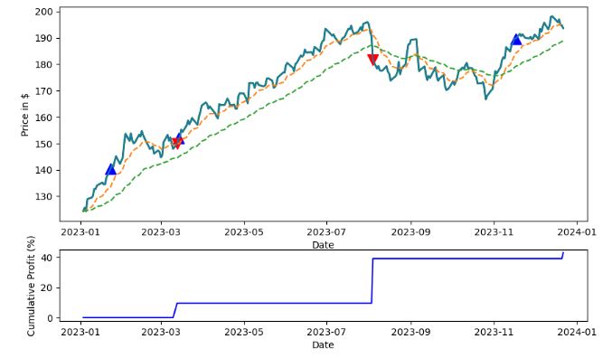
- It looks like the APO trading strategy yields the cumulative return ca. 40%.
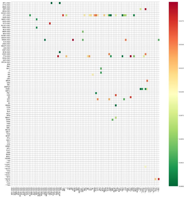
Cointegrated Pairs of Stocks
- Let’s implement the pair trading strategy by downloading the crypto Forex stocks, bank stocks, and global indexes
import numpy as np
import pandas as pd
import matplotlib.pyplot as plt

import warnings
warnings.filterwarnings("ignore")


import yfinance as yf
from analysis_utils2 import calculate_profit, load_ticker_ts_df, plot_strategy

crypto_forex_stocks = ['BTC-USD', 'ETH-USD', 'BNB-USD', 'XRP-USD', 'ADA-USD', 'DOGE-USD', 'ETC-USD', 'XLM-USD', 'AAVE-USD', 'EOS-USD', 'XTZ-USD', 'ALGO-USD', 'XMR-USD', 'KCS-USD',
                       'MKR-USD', 'BSV-USD', 'RUNE-USD', 'DASH-USD', 'KAVA-USD', 'ICX-USD', 'LINA-USD', 'WAXP-USD', 'LSK-USD', 'EWT-USD', 'XCN-USD', 'HIVE-USD', 'FTX-USD', 'RVN-USD', 'SXP-USD', 'BTCB-USD']
bank_stocks = ['JPM', 'BAC', 'WFC', 'C', 'GS', 'MS', 'DB', 'UBS', 'BBVA', 'SAN', 'ING', ' BNPQY', 'HSBC', 'SMFG', 'PNC', 'USB', 'BK', 'STT', 'KEY', 'RF', 'HBAN', 'FITB',  'CFG',
               'BLK', 'ALLY', 'MTB', 'NBHC', 'ZION', 'FFIN', 'FHN', 'UBSI', 'WAL', 'PACW', 'SBCF', 'TCBI', 'BOKF', 'PFG', 'GBCI', 'TFC', 'CFR', 'UMBF', 'SPFI', 'FULT', 'ONB', 'INDB', 'IBOC', 'HOMB']
global_indexes = ['^DJI', '^IXIC', '^GSPC', '^FTSE', '^N225', '^HSI', '^AXJO', '^KS11', '^BFX', '^N100',
                  '^RUT', '^VIX', '^TNX']

START_DATE = '2023-01-01'
END_DATE = '2023-12-24'

universe_tickers = crypto_forex_stocks + bank_stocks + global_indexes
universe_tickers_ts_map = {ticker: load_ticker_ts_df(
    ticker, START_DATE, END_DATE) for ticker in universe_tickers}


def sanitize_data(data_map):
    TS_DAYS_LENGTH = (pd.to_datetime(END_DATE) -
                      pd.to_datetime(START_DATE)).days
    data_sanitized = {}

    date_range = pd.date_range(start=START_DATE, end=END_DATE, freq='D')
    for ticker, data in data_map.items():
        if data is None or len(data) < (TS_DAYS_LENGTH / 2):
            # We cannot handle shorter TSs
            continue

        if len(data) > TS_DAYS_LENGTH:
            # Normalize to have the same length (TS_DAYS_LENGTH)
            data = data[-TS_DAYS_LENGTH:]

        # Reindex the time series to match the date range and fill in any blanks (Not Numbers)
        data = data.reindex(date_range)
        data['Adj Close'].replace([np.inf, -np.inf], np.nan, inplace=True)
        data['Adj Close'].interpolate(method='linear', inplace=True)
        data['Adj Close'].fillna(method='pad', inplace=True)
        data['Adj Close'].fillna(method='bfill', inplace=True)

        assert not np.any(np.isnan(data['Adj Close'])) and not np.any(
            np.isinf(data['Adj Close']))

        data_sanitized[ticker] = data

    return data_sanitized


# Sample some
uts_sanitized = sanitize_data(universe_tickers_ts_map)
uts_sanitized['JPM'].shape, uts_sanitized['BTC-USD'].shape
((358, 6), (358, 6))
- Finding and plotting cointegrated pairs
from statsmodels.tsa.stattools import coint
from itertools import combinations
from statsmodels.tsa.stattools import coint


def find_cointegrated_pairs(tickers_ts_map, p_value_threshold=0.2):
    """
    Find cointegrated pairs of stocks based on the Augmented Dickey-Fuller (ADF) test.
    Parameters:
    - tickers_ts_map (dict): A dictionary where keys are stock tickers and values are time series data.
    - p_value_threshold (float): The significance level for cointegration testing.
    Returns:
    - pvalue_matrix (numpy.ndarray): A matrix of cointegration p-values between stock pairs.
    - pairs (list): A list of tuples representing cointegrated stock pairs and their p-values.
    """
    tickers = list(tickers_ts_map.keys())
    n = len(tickers)

    # Extract 'Adj Close' prices into a matrix (each column is a time series)
    adj_close_data = np.column_stack(
        [tickers_ts_map[ticker]['Adj Close'].values for ticker in tickers])
    pvalue_matrix = np.ones((n, n))

    # Calculate cointegration p-values for unique pair combinations
    for i, j in combinations(range(n), 2):
        result = coint(adj_close_data[:, i], adj_close_data[:, j])
        pvalue_matrix[i, j] = result[1]
    pairs = [(tickers[i], tickers[j], pvalue_matrix[i, j])
             for i, j in zip(*np.where(pvalue_matrix < p_value_threshold))]

    return pvalue_matrix, pairs


# This section can take up to 5mins
P_VALUE_THRESHOLD = 0.02
pvalues, pairs = find_cointegrated_pairs(
    uts_sanitized, p_value_threshold=P_VALUE_THRESHOLD)
import seaborn as sns

plt.figure(figsize=(24, 24))
heatmap = sns.heatmap(pvalues, xticklabels=uts_sanitized.keys(),
                      yticklabels=uts_sanitized.keys(), cmap='RdYlGn_r',
                      mask=(pvalues > (P_VALUE_THRESHOLD)),
                      linecolor='gray', linewidths=0.5)
heatmap.set_xticklabels(heatmap.get_xticklabels(), size=12)
heatmap.set_yticklabels(heatmap.get_yticklabels(), size=12)
plt.show()
- Plotting cointegration P-values 0-10 (in 1000s)
sorted_pairs = sorted(pairs, key=lambda x: x[2], reverse=False)
sorted_pairs = sorted_pairs[0:35]
sorted_pairs_labels, pairs_p_values = zip(
    *[(f'{y1} <-> {y2}', p*1000) for y1, y2, p in sorted_pairs])

plt.figure(figsize=(12, 18))
plt.barh(sorted_pairs_labels,
         pairs_p_values, color='red')
plt.xlabel('P-Values (1000)', fontsize=8)
plt.ylabel('Pairs', fontsize=6)
plt.title('Cointegration P-Values (in 1000s)', fontsize=20)

plt.grid(axis='both', linestyle='--', alpha=0.7)
plt.show()
plt.savefig('pairs_pvalue.png')
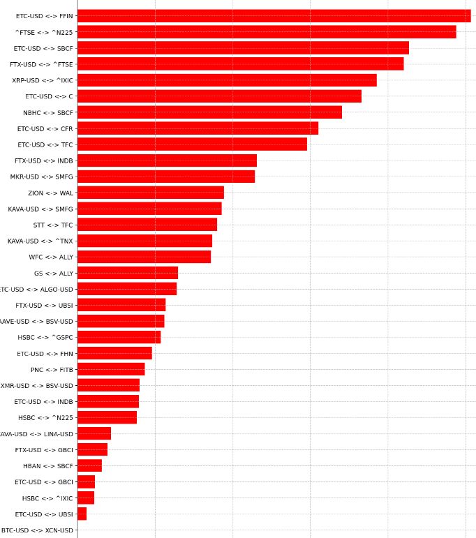
P-Values 0-10 (1000)
- Comparing the following ticker pairs with highest correlations
from sklearn.preprocessing import MinMaxScaler

ticker_pairs = [("FTX-USD", "INDB"), ("ZION", "WAL"), ("GS", "ALLY")]

fig, axs = plt.subplots(3, 1, figsize=(12, 10))
scaler = MinMaxScaler()

for i, (ticker1, ticker2) in enumerate(ticker_pairs):
    # Scale the price data for each pair using MIN MAX
    scaled_data1 = scaler.fit_transform(
        uts_sanitized[ticker1]['Adj Close'].values.reshape(-1, 1))
    scaled_data2 = scaler.fit_transform(
        uts_sanitized[ticker2]['Adj Close'].values.reshape(-1, 1))

    axs[i].plot(scaled_data1, label=f'{ticker1}', color='lightgray', alpha=0.7,lw=2)
    axs[i].plot(scaled_data2, label=f'{ticker2}', color='lightgray', alpha=0.7,lw=2)

    # Apply rolling mean with a window of 15
    scaled_data1_smooth = pd.Series(scaled_data1.flatten()).rolling(
        window=15, min_periods=1).mean()
    scaled_data2_smooth = pd.Series(scaled_data2.flatten()).rolling(
        window=15, min_periods=1).mean()

    axs[i].plot(scaled_data1_smooth, label=f'{ticker1} SMA', color='red')
    axs[i].plot(scaled_data2_smooth, label=f'{ticker2} SMA', color='blue')

    axs[i].set_ylabel('*Scaled* Price $', fontsize=12)
    axs[i].set_title(f'{ticker1} vs {ticker2}', fontsize=18)
    axs[i].legend()
    axs[i].set_xticks([])

plt.tight_layout()
plt.show()
![Comparing the ticker pairs [("FTX-USD", "INDB"), ("ZION", "WAL"), ("GS", "ALLY")]](https://newdigitals.org/wp-content/uploads/2023/12/invest_ftx.jpg?w=730)
Z-Score vs Trading Signals
- Let’s create trading signals using the Z-score and mean.
- Plotting FTX-USD / INDB: Price Ratio and Z-Score
TRAIN = int(len(uts_sanitized["FTX-USD"]) * 0.80)
TEST = len(uts_sanitized["FTX-USD"]) - TRAIN

AAVE_ts = uts_sanitized["FTX-USD"]["Adj Close"][:TRAIN]
C_ts = uts_sanitized["INDB"]["Adj Close"][:TRAIN]

ratios = C_ts/AAVE_ts
fig, ax = plt.subplots(figsize=(10, 6))

ratios_mean = np.mean(ratios)
ratios_std = np.std(ratios)
ratios_zscore = (ratios - ratios_mean) / ratios_std

ax.plot(ratios.index, ratios_zscore, label="Z-Score", color='blue')

# Plot reference lines
ax.axhline(1.0, color="green", linestyle='--', label="Upper Threshold (1.0)")
ax.axhline(-1.0, color="red", linestyle='--', label="Lower Threshold (-1.0)")
ax.axhline(0, color="black", linestyle='--', label="Baseline")

ax.set_title('FTX-USD / INDB: Price Ratio and Z-Score', fontsize=18)
ax.set_xlabel('Date',fontsize=14)
ax.set_ylabel('Price Ratio / Z-Score',fontsize=14)
ax.legend()
plt.tight_layout()
plt.show()
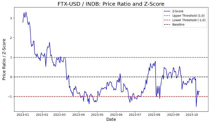
- The green horizontal line here will signal a buy for INDB if crossed and a sell for FTX-USD, the red line will do the opposite.
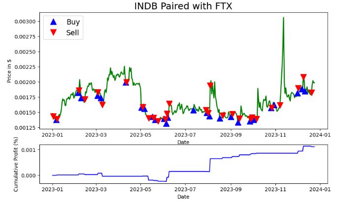
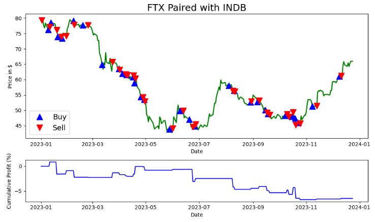
- Generating and plotting trading signals based on the Z-score analysis and the price ratio between FTX-USD and INDB
def signals_zscore_evolution(ticker1_ts, ticker2_ts, window_size=15, first_ticker=True):
    """
    Generate trading signals based on z-score analysis of the ratio between two time series.
    Parameters:
    - ticker1_ts (pandas.Series): Time series data for the first security.
    - ticker2_ts (pandas.Series): Time series data for the second security.
    - window_size (int): The window size for calculating z-scores and ratios' statistics.
    - first_ticker (bool): Set to True to use the first ticker as the primary signal source, and False to use the second.

    Returns:
    - signals_df (pandas.DataFrame): A DataFrame with 'signal' and 'orders' columns containing buy (1) and sell (-1) signals.

    """
    ratios = ticker1_ts / ticker2_ts

    ratios_mean = ratios.rolling(
        window=window_size, min_periods=1, center=False).mean()
    ratios_std = ratios.rolling(
        window=window_size, min_periods=1, center=False).std()

    z_scores = (ratios - ratios_mean) / ratios_std

    buy = ratios.copy()
    sell = ratios.copy()

    if first_ticker:
        # These are empty zones, where there should be no signal
        # the rest is signalled by the ratio.
        buy[z_scores > -1] = 0
        sell[z_scores < 1] = 0
    else:
        buy[z_scores < 1] = 0
        sell[z_scores > -1] = 0

    signals_df = pd.DataFrame(index=ticker1_ts.index)
    signals_df['signal'] = np.where(buy > 0, 1, np.where(sell < 0, -1, 0))
    signals_df['orders'] = signals_df['signal'].diff()
    signals_df.loc[signals_df['orders'] == 0, 'orders'] = None

    return signals_df

AAVE_ts = uts_sanitized["FTX-USD"]["Adj Close"]
C_ts = uts_sanitized["INDB"]["Adj Close"]

#plt.figure(figsize=(10, 6))
signals_df1 = signals_zscore_evolution(AAVE_ts, C_ts)
profit_df1 = calculate_profit(signals_df1, AAVE_ts)
ax1, _ = plot_strategy(AAVE_ts, signals_df1, profit_df1)

signals_df2 = signals_zscore_evolution(AAVE_ts, C_ts, first_ticker=False)
profit_df2 = calculate_profit(signals_df2, C_ts)
ax2, _ = plot_strategy(C_ts, signals_df2, profit_df2)

ax1.legend(loc='upper left', fontsize=14)
ax1.set_title(f'INDB Paired with FTX', fontsize=18)
ax2.legend(loc='lower left', fontsize=14)
ax2.set_title(f'FTX Paired with INDB', fontsize=18)
plt.tight_layout()
plt.show()
- Plotting FTX & INDB Paired – Cumulative Profit
plt.figure(figsize=(10, 6))
cumulative_profit_combined = profit_df1 + profit_df2
ax2_combined = cumulative_profit_combined.plot(
    label='Profit%', color='green')
plt.legend(loc='lower left', fontsize=14)
plt.title(f'FTX & INDB Paired - Cumulative Profit', fontsize=18)
plt.tight_layout()
plt.show()
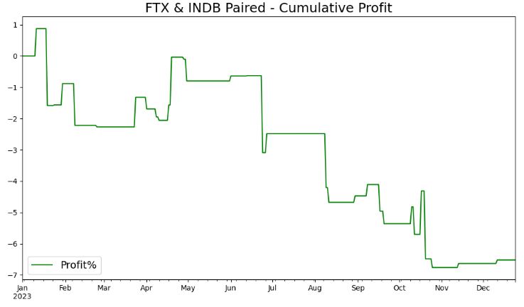
- It is clear that this trading strategy is not profitable in ’23.
Conclusions
- In this study, we focused on mitigating market risk while constructing market-neutral portfolios. In a situation where financial markets are characterized by high volatility, such portfolios are more likely to outperform other strategies.
- Quantitative analysis plays a critical role in market-neutral trading by providing traders with a data-driven approach to identifying pricing discrepancies and making investment decisions. This is performed with algorithms and statistical models to analyze large amounts of historical data and identify patterns and relationships in the market.
- Statistical arbitrage (aka Stat-Arb) was chosen to be the core trading strategy that seeks to profit from discrepancies in the prices of related securities.
- A mean-reversion statistical arbitrage strategy was implemented as pairs trading. Pairs trading involves identifying two securities that have a high correlation and taking positions in the hope that the prices of the two securities will eventually converge.
- A popular example of pairs trading: if the prices of two stocks have historically moved in tandem, and one of them suddenly drops in price, the trader could buy the undervalued stock and short sell the overvalued one.
- We addressed the problem of Markowitz portfolio optimization for a one-year horizon investment, through the pairs trading cointegrated strategy. Such a strategy allowed us to identify the prices and returns of each stock on the basis of a cointegration relationship estimated by means of EMA and the covariance ratios between stock pairs.
- We assessed the viability of our portfolios by means of backtesting while adding the Market Capital Line (MCL) to the efficient frontier of simulated trading in terms of max Sharpe ratio and min variance.
- We experimented with the investors choices of risk/reward, through indifference curves and descriptive statistics of cumulative returns.
- We compared our findings to the results of technical analysis by generating the double SMA/EMA strategy, mean reversion trading signals, naive momentum, and APO thresholds.
- We also created trading signals using the Z-score and mean.
- We examined asset allocation across a number of sectors including technology, financial services, and industrials in 2023.
- We checked correlations with AAPL, performed AAPL Stat-Arb 1Y backtesting, and constructed portfolio efficient frontiers by adding MCL, MVP, and TAN to simulated trades.
- We implemented the pair trading strategy by downloading the crypto Forex stocks, bank stocks, and global indexes.
- We believe the present diversified approach improves the market-neutral landscape by providing a set of optimal portfolios that offer the highest expected return for a defined level of risk or the lowest risk for a given level of expected return.
- Market-neutral trading is an evolving strategy. Following best practices and the present study, we prefer to focus on using statistical models and growth factors rather than fundamental arbitrage, as technology makes it easier to gain access to huge data and analyze them. However, regulatory changes and increased competition in the market could also impact the future of market-neutral trading.
Explore More
- A Comprehensive Analysis of Best Trading Technical Indicators w/ TA-Lib – Tesla ’23
- Real-Time Stock Sentiment Analysis w/ NLP Web Scraping
- Plotly Dash TA Stock Market App
- Optimizing NVIDIA Returns-Drawdowns MVA Crossovers vs Simple RNN Mean Reversal Trading Strategies in Python
- Multiple-Criteria Technical Analysis of Blue Chips in Python
- 360-Deg Revision of Risk Aware Investing after SVB Collapse – 1. The Financial Sector
- Towards Max(ROI/Risk) Trading
- Portfolio max(Return/Risk) Stochastic Optimization of 20 Dividend Growth Stocks
- Risk-Return Analysis and LSTM Price Predictions of 4 Major Tech Stocks in 2023
- The Donchian Channel vs Buy-and-Hold Breakout Trading Systems – $MO Use-Case
- Applying a Risk-Aware Portfolio Rebalancing Strategy to ETF, Energy, Pharma, and Aerospace/Defense Stocks in 2023
- Advanced Integrated Data Visualization (AIDV) in Python – 1. Stock Technical Indicators
- Quant Trading using Monte Carlo Predictions and 62 AI-Assisted Trading Technical Indicators (TTI)
- The Qullamaggie’s OXY Swing Breakouts
- The Qullamaggie’s TSLA Breakouts for Swing Traders
- Stock Portfolio Risk/Return Optimization
- Risk/Return QC via Portfolio Optimization – Current Positions of The Dividend Breeder
- Portfolio Optimization Risk/Return QC – Positions of Humble Div vs Dividend Glenn
- Oracle Monte Carlo Stock Simulations
- Predicting the JPM Stock Price and Breakouts with Auto ARIMA, FFT, LSTM and Technical Trading Indicators
- Bear vs. Bull Portfolio Risk/Return Optimization QC Analysis
- A TradeSanta’s Quick Guide to Best Swing Trading Indicators
- Top 6 Reliability/Risk Engineering Learnings
- Bear Market Similarity Analysis using Nasdaq 100 Index Data
- Are Blue Chips Perfect for This Bear Market?
- DJI Market State Analysis using the Cruz Fitting Algorithm
- The CodeX-Aroon Auto-Trading Approach – the AAPL Use Case
- AAPL Stock Technical Analysis 2 June 2022
- Risk-Aware Strategies for DCA Investors
- Inflation-Resistant Stocks to Buy


One-Time
Monthly
Yearly
Make a one-time donation
Make a monthly donation
Make a yearly donation
Choose an amount
€5.00
€15.00
€100.00
€5.00
€15.00
€100.00
€5.00
€15.00
€100.00
Or enter a custom amount
€
Your contribution is appreciated.
Your contribution is appreciated.
Your contribution is appreciated.
DonateDonate monthlyDonate yearly
Leave a comment