
- The objective of this project is to predict the Remaining Useful Life (RUL) of NASA turbofan jet engines by comparing the statsmodels OLS, ML SciKit-Learn regression vs LSTM Keras in Python. RUL is equivalent of number of flights remained for the engine after the last data point in the test dataset.
- An important requirement for the damage modeling process was the availability of a suitable system model that allows input variations of health related parameters and recording of the resulting output sensor measurements. The recently released C-MAPSS (Commercial Modular Aero- Propulsion System Simulation) meets these requirements and was chosen for this work. C-MAPSS is a tool for simulating a realistic large commercial turbofan engine.
- The input dataset is the Kaggle version of the public dataset for asset degradation modeling from NASA. It includes Run-to-Failure simulated data from turbo fan jet engines.
- The dataset consists of multiple multivariate time series. Each data set is further divided into training and test subsets. Each time series is from a different engine i.e., the data can be considered to be from a fleet of engines of the same type. Each engine starts with different degrees of initial wear and manufacturing variation which is unknown to the user.
- Nasa Turbofan Engine Remaining Lifetime

Data Preparation & Exploration
- Let’s set the working directory YOURPATH and import key libraries
import os
os.chdir('YOURPATH')
os. getcwd()
import numpy as np
import pandas as pd

from IPython.display import display, HTML
import plotly.graph_objects as go
import plotly.express as px
from plotly.subplots import make_subplots
import plotly.io as pio


import seaborn as sns
from importlib import reload
import matplotlib.pyplot as plt
import matplotlib
import warnings
- Reading the input data and giving names to the features
index_names = ['engine', 'cycle']
setting_names = ['setting_1', 'setting_2', 'setting_3']
sensor_names=[ "(Fan inlet temperature) (◦R)",
"(LPC outlet temperature) (◦R)",
"(HPC outlet temperature) (◦R)",
"(LPT outlet temperature) (◦R)",
"(Fan inlet Pressure) (psia)",
"(bypass-duct pressure) (psia)",
"(HPC outlet pressure) (psia)",
"(Physical fan speed) (rpm)",
"(Physical core speed) (rpm)",
"(Engine pressure ratio(P50/P2)",
"(HPC outlet Static pressure) (psia)",
"(Ratio of fuel flow to Ps30) (pps/psia)",
"(Corrected fan speed) (rpm)",
"(Corrected core speed) (rpm)",
"(Bypass Ratio) ",
"(Burner fuel-air ratio)",
"(Bleed Enthalpy)",
"(Required fan speed)",
"(Required fan conversion speed)",
"(High-pressure turbines Cool air flow)",
"(Low-pressure turbines Cool air flow)" ]
col_names = index_names + setting_names + sensor_names

df_train = pd.read_csv(('train_FD001.txt'), sep='\s+', header=None, names=col_names)
df_test = pd.read_csv(('test_FD001.txt'), sep='\s+', header=None, names=col_names)
df_test_RUL = pd.read_csv(('RUL_FD001.txt'), sep='\s+', header=None, names=['RUL'])
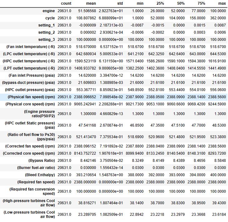
- The general information about the dataset is as follows:
df_train.info()
<class 'pandas.core.frame.DataFrame'>
RangeIndex: 20631 entries, 0 to 20630
Data columns (total 26 columns):
 #   Column                                   Non-Null Count  Dtype
---  ------                                   --------------  -----
 0   engine                                   20631 non-null  int64
 1   cycle                                    20631 non-null  int64
 2   setting_1                                20631 non-null  float64
 3   setting_2                                20631 non-null  float64
 4   setting_3                                20631 non-null  float64
 5   (Fan inlet temperature) (◦R)             20631 non-null  float64
 6   (LPC outlet temperature) (◦R)            20631 non-null  float64
 7   (HPC outlet temperature) (◦R)            20631 non-null  float64
 8   (LPT outlet temperature) (◦R)            20631 non-null  float64
 9   (Fan inlet Pressure) (psia)              20631 non-null  float64
 10  (bypass-duct pressure) (psia)            20631 non-null  float64
 11  (HPC outlet pressure) (psia)             20631 non-null  float64
 12  (Physical fan speed) (rpm)               20631 non-null  float64
 13  (Physical core speed) (rpm)              20631 non-null  float64
 14  (Engine pressure ratio(P50/P2)           20631 non-null  float64
 15  (HPC outlet Static pressure) (psia)      20631 non-null  float64
 16  (Ratio of fuel flow to Ps30) (pps/psia)  20631 non-null  float64
 17  (Corrected fan speed) (rpm)              20631 non-null  float64
 18  (Corrected core speed) (rpm)             20631 non-null  float64
 19  (Bypass Ratio)                           20631 non-null  float64
 20  (Burner fuel-air ratio)                  20631 non-null  float64
 21  (Bleed Enthalpy)                         20631 non-null  int64
 22  (Required fan speed)                     20631 non-null  int64
 23  (Required fan conversion speed)          20631 non-null  float64
 24  (High-pressure turbines Cool air flow)   20631 non-null  float64
 25  (Low-pressure turbines Cool air flow)    20631 non-null  float64
dtypes: float64(22), int64(4)
memory usage: 4.1 MB

df_train.shape
(20631, 26)

df_test.shape
(13096, 26)
df_train.describe().T
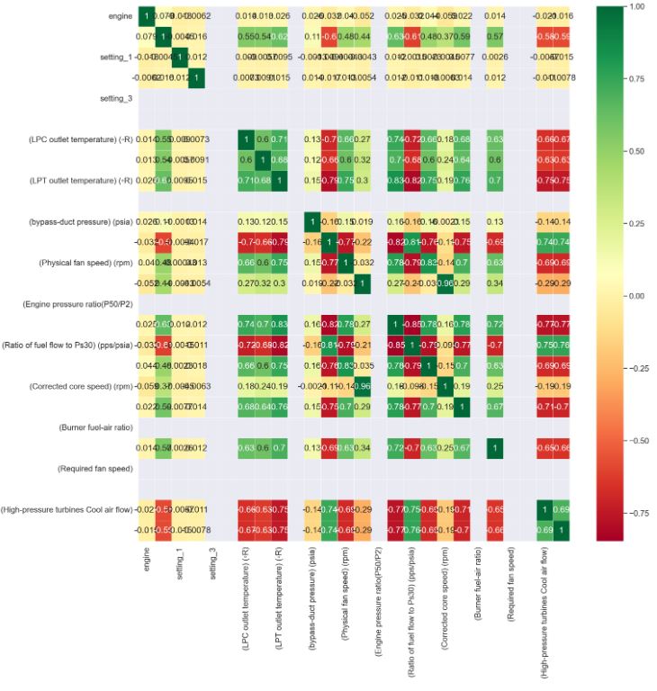
- Plotting the correlation heatmap
sns.heatmap(df_train.corr(),annot=True,cmap='RdYlGn',linewidths=0.2)
sns.set(font_scale=1.2)
fig=plt.gcf()
fig.set_size_inches(16,16)
plt.show()
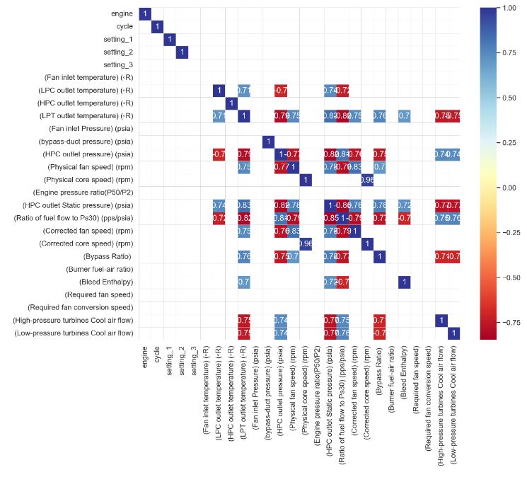
- Plotting the correlation heatmap with threshold = 0.70
plt.figure(figsize=(12,10))
sns.set(font_scale=1.1)
threshold = 0.70
sns.set_style("whitegrid", {"axes.facecolor": ".0"})
df_cluster2 = df_train.corr()
mask = df_cluster2.where((abs(df_cluster2) >= threshold)).isna()
plot_kws={"s": 1}
sns.heatmap(df_cluster2,
            cmap='RdYlBu',
            annot=True,
            mask=mask,
            linewidths=0.2,
            linecolor='lightgrey').set_facecolor('white')
- Dropping the sensors with constant values
sens_const_values = []
for feature in list(setting_names + sensor_names):
    try:
        if df_train[feature].min()==df_train[feature].max():
            sens_const_values.append(feature)
    except:
        pass

print(sens_const_values)
df_train.drop(sens_const_values,axis=1,inplace=True)
df_test.drop(sens_const_values,axis=1,inplace=True)

['setting_3', '(Fan inlet temperature) (◦R)', '(Fan inlet Pressure) (psia)', '(Engine pressure ratio(P50/P2)', '(Burner fuel-air ratio)', '(Required fan speed)', '(Required fan conversion speed)']
- Dropping highly correlated features with threshold > 0.95
# drop all but one of the highly correlated features
cor_matrix = df_train.corr().abs()
upper_tri = cor_matrix.where(np.triu(np.ones(cor_matrix.shape),k=1).astype(np.bool))
corr_features = [column for column in upper_tri.columns if any(upper_tri[column] > 0.95)]
print(corr_features)
df_train.drop(corr_features,axis=1,inplace=True)
df_test.drop(corr_features,axis=1,inplace=True)

['(Corrected core speed) (rpm)']
- Creating the list of features
features = list(df_train.columns)
list(df_train)

['engine',
 'cycle',
 'setting_1',
 'setting_2',
 '(LPC outlet temperature) (◦R)',
 '(HPC outlet temperature) (◦R)',
 '(LPT outlet temperature) (◦R)',
 '(bypass-duct pressure) (psia)',
 '(HPC outlet pressure) (psia)',
 '(Physical fan speed) (rpm)',
 '(Physical core speed) (rpm)',
 '(HPC outlet Static pressure) (psia)',
 '(Ratio of fuel flow to Ps30) (pps/psia)',
 '(Corrected fan speed) (rpm)',
 '(Bypass Ratio) ',
 '(Bleed Enthalpy)',
 '(High-pressure turbines Cool air flow)',
 '(Low-pressure turbines Cool air flow)']
- Checking for missing data
# check for missing data
for feature in features:
    print(feature + " - " + str(len(df_train[df_train[feature].isna()])))

engine - 0
cycle - 0
setting_1 - 0
setting_2 - 0
(LPC outlet temperature) (◦R) - 0
(HPC outlet temperature) (◦R) - 0
(LPT outlet temperature) (◦R) - 0
(bypass-duct pressure) (psia) - 0
(HPC outlet pressure) (psia) - 0
(Physical fan speed) (rpm) - 0
(Physical core speed) (rpm) - 0
(HPC outlet Static pressure) (psia) - 0
(Ratio of fuel flow to Ps30) (pps/psia) - 0
(Corrected fan speed) (rpm) - 0
(Bypass Ratio)  - 0
(Bleed Enthalpy) - 0
(High-pressure turbines Cool air flow) - 0
(Low-pressure turbines Cool air flow) - 0
- Defining the maximum life for each engine
# define the maximum life of each engine, as this could be used to obtain the RUL at each point in time of the engine's life
df_train_RUL = df_train.groupby(['engine']).agg({'cycle':'max'})
df_train_RUL.rename(columns={'cycle':'life'},inplace=True)
df_train_RUL.head()

	life
engine
1	192
2	287
3	179
4	189
5	269
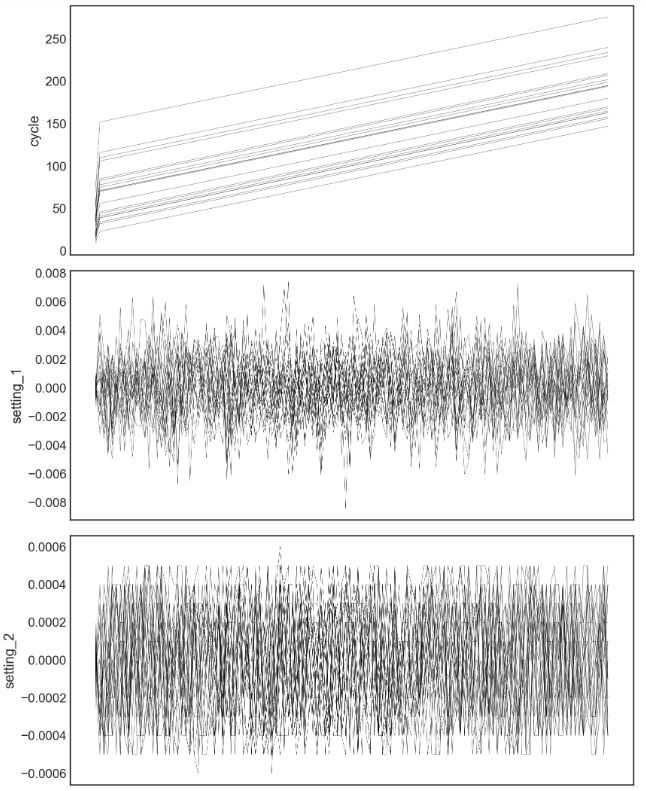
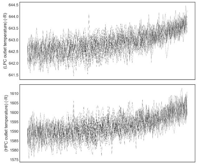
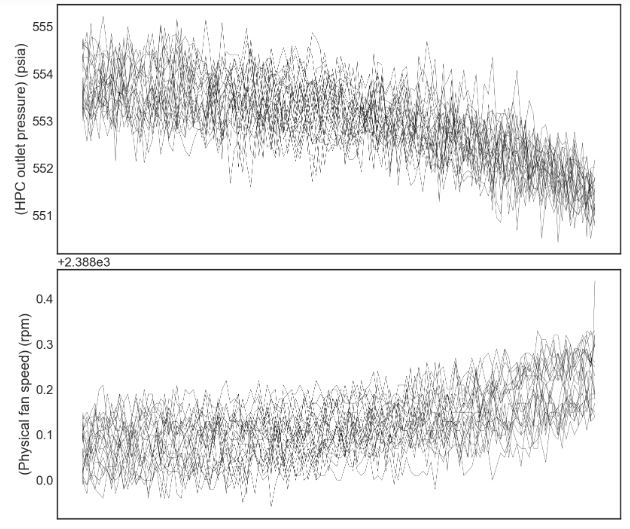
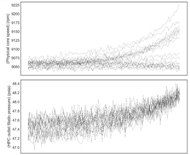
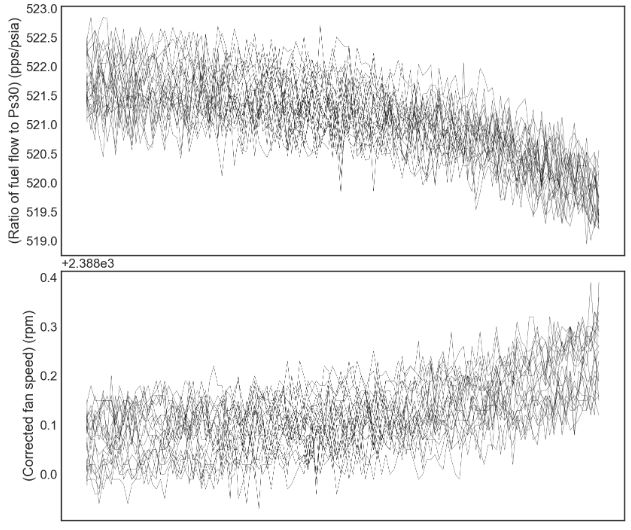
- Creating and plotting the training dataset with RUL>125
df_train=df_train.merge(df_train_RUL,how='left',on=['engine'])

df_train['RUL']=df_train['life']-df_train['cycle']
df_train.drop(['life'],axis=1,inplace=True)

# the RUL prediction is only useful nearer to the end of the engine's life, therefore we put an upper limit on the RUL
# this is a bit sneaky, since it supposes that the test set has RULs of less than this value, the closer you are
# to the true value, the more accurate the model will be
df_train['RUL'][df_train['RUL']>125]=125
#df_train.head()
plt.style.use('seaborn-white')
from IPython.core.display import display, HTML
display(HTML("<style>div.output_scroll { height: 144em; }</style>"))
plt.rcParams['figure.figsize']=8,60
plt.rcParams['font.family'] = 'sans-serif'
plt.rcParams['font.size'] = 4
plt.rcParams['lines.linewidth'] = 0.2
plot_items = list(df_train.columns)[1:-1]
fig,ax = plt.subplots(len(plot_items),sharex=True)
fig.tight_layout()
fig.subplots_adjust(wspace=1.5)
ax[0].invert_xaxis()

engines = list(df_train['engine'].unique())

for engine in engines[10:30]:
    for i,item in enumerate(plot_items):
        f = sns.lineplot(data=df_train[df_train['engine']==engine],x='RUL',y=item,color='black',ax=ax[i],
                        )


OLS & SciKit-Learn Regression
- Implementing the OLS backward regression
Selected_Features = []
import statsmodels.api as sm

def backward_regression(X, y, initial_list=[], threshold_out=0.05, verbose=True):
    """To select feature with Backward Stepwise Regression

    Args:
        X -- features values
        y -- target variable
        initial_list -- features header
        threshold_out -- pvalue threshold of features to drop
        verbose -- true to produce lots of logging output

    Returns:
        list of selected features for modeling
    """
    included = list(X.columns)
    while True:
        changed = False
        model = sm.OLS(y, sm.add_constant(pd.DataFrame(X[included]))).fit()
        # use all coefs except intercept
        pvalues = model.pvalues.iloc[1:]
        worst_pval = pvalues.max()  # null if pvalues is empty
        if worst_pval > threshold_out:
            changed = True
            worst_feature = pvalues.idxmax()
            included.remove(worst_feature)
            if verbose:
                print(f"worst_feature : {worst_feature}, {worst_pval} ")
        if not changed:
            break
    Selected_Features.append(included)
    print(f"\nSelected Features:\n{Selected_Features[0]}")


# Application of the backward regression function on our training data
X = df_train.iloc[:,1:-1]
y = df_train.iloc[:,-1]
backward_regression(X, y)

worst_feature : setting_1, 0.3590854598718034
worst_feature : setting_2, 0.18806323578786557

Selected Features:
['cycle', '(LPC outlet temperature) (◦R)', '(HPC outlet temperature) (◦R)', '(LPT outlet temperature) (◦R)', '(bypass-duct pressure) (psia)', '(HPC outlet pressure) (psia)', '(Physical fan speed) (rpm)', '(Physical core speed) (rpm)', '(HPC outlet Static pressure) (psia)', '(Ratio of fuel flow to Ps30) (pps/psia)', '(Corrected fan speed) (rpm)', '(Bypass Ratio) ', '(Bleed Enthalpy)', '(High-pressure turbines Cool air flow)', '(Low-pressure turbines Cool air flow)']

feature_names = Selected_Features[0]
np.shape(X)
(20631, 17)
len(feature_names)
15
- Implementing the core ML performance metrics
import time
model_performance = pd.DataFrame(columns=['r-Squared','RMSE','total time'])

from sklearn.model_selection import train_test_split
from sklearn.metrics import mean_squared_error
from sklearn.metrics import make_scorer, accuracy_score

import sklearn
from sklearn.metrics import mean_squared_error, r2_score
# from sklearn.ensemble import RandomForestRegressor

model_performance = pd.DataFrame(columns=['R2','RMSE', 'time to train','time to predict','total time'])


def R_squared(y_true, y_pred):
    SS_res =  K.sum(K.square(y_true - y_pred))
    SS_tot = K.sum(K.square(y_true - K.mean(y_true)))
    return 1 - SS_res/(SS_tot + K.epsilon())

from sklearn.metrics import mean_absolute_error
from sklearn.metrics import r2_score
from sklearn.metrics import mean_squared_error
- Performing train/test data preparation
df_test_cycle = df_test.groupby(['engine']).agg({'cycle':'max'})
df_test_cycle.rename(columns={'cycle':'life'},inplace=True)
df_test_max = df_test.merge(df_test_cycle,how='left',on=['engine'])
df_test_max = df_test_max[(df_test_max['cycle']==df_test_max['life'])]
df_test_max.drop(['life'],axis=1,inplace=True)

X_train = df_train[feature_names]
y_train = df_train.iloc[:,-1]
X_test = df_test_max[feature_names]
y_test = df_test_RUL.iloc[:,-1]

from sklearn.preprocessing import MinMaxScaler
sc = MinMaxScaler()
X_train = sc.fit_transform(X_train)
X_test = sc.transform(X_test)
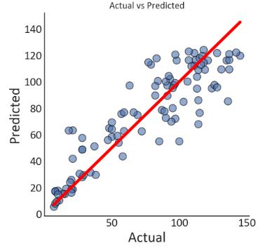
- Training the KNeighborsRegressor model
%%time
from sklearn.neighbors import KNeighborsRegressor
start = time.time()
model = KNeighborsRegressor(n_neighbors=9).fit(X_train,y_train)
end_train = time.time()
y_predictions = model.predict(X_test) # These are the predictions from the test data.
end_predict = time.time()


model_performance.loc['kNN'] = [model.score(X_test,y_test),
                                   mean_squared_error(y_test,y_predictions,squared=False),
                                   end_train-start,
                                   end_predict-end_train,
                                   end_predict-start]

print('R-squared error: '+ "{:.2%}".format(model.score(X_test,y_test)))
print('Root Mean Squared Error: '+ "{:.2f}".format(mean_squared_error(y_test,y_predictions,squared=False)))

R-squared error: 79.79%
Root Mean Squared Error: 18.68
CPU times: total: 188 ms
Wall time: 296 ms
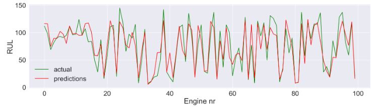
- Plotting the output of KNeighborsRegressor test prediction
plt.style.use('seaborn-white')
plt.rcParams['figure.figsize']=5,5
plt.rcParams['font.family'] = 'Calibri'
plt.rcParams['lines.linewidth'] = 3
plt.rcParams['axes.labelsize']=20
plt.rcParams['xtick.labelsize']=16
plt.rcParams['ytick.labelsize']=16
plt.rcParams['legend.fontsize']=16

fig,ax = plt.subplots()
plt.title('Actual vs Predicted')
plt.xlabel('Actual')
plt.ylabel('Predicted')
g = sns.scatterplot(x=y_test,
                y=y_predictions,
                s=100,
                alpha=0.6,
                linewidth=1,
                edgecolor='black',
                ax=ax)
f = sns.lineplot(x=[min(y_test),max(y_test)],
             y=[min(y_test),max(y_test)],
             linewidth=4,
             color='red',
             ax=ax)

plt.annotate(text=('R-squared error: '+ "{:.2%}".format(model.score(X_test,y_test)) +'\n' +
                  'Root Mean Squared Error: '+ "{:.2f}".format(mean_squared_error(y_test,y_predictions,squared=False))),
             xy=(0,150),
             size='medium')

xlabels = ['{:,.0f}'.format(x) for x in g.get_xticks()]
g.set_xticklabels(xlabels)
ylabels = ['{:,.0f}'.format(x) for x in g.get_yticks()]
g.set_yticklabels(ylabels)
sns.despine()
plt.style.use('seaborn-white')
plt.rcParams['figure.figsize']=20,5
sns.set(font_scale=2)

fig,ax = plt.subplots()
plt.ylabel('RUL')
plt.xlabel('Engine nr')

g = sns.lineplot(x = np.arange(0,len(df_train['engine'].unique())),
                y=y_test,
                color='green',
                label = 'actual',
                ax=ax)

f = sns.lineplot(x = np.arange(0,len(df_train['engine'].unique())),
                y=y_predictions,
                color='red',
                label = 'predictions',
                ax=ax)
ax.legend()
- Training the SVR model
%%time
from sklearn.svm import SVR
start = time.time()
model = SVR(kernel="rbf", C=100, gamma=0.5, epsilon=0.01).fit(X_train,y_train)
end_train = time.time()
y_predictions = model.predict(X_test) # These are the predictions from the test data.
end_predict = time.time()
model_performance.loc['SVM'] = [model.score(X_test,y_test),
mean_squared_error(y_test,y_predictions,squared=False),
end_train-start,
end_predict-end_train,
end_predict-start]
print('R-squared error: '+ "{:.2%}".format(model.score(X_test,y_test)))
print('Root Mean Squared Error: '+ "{:.2f}".format(mean_squared_error(y_test,y_predictions,squared=False)))
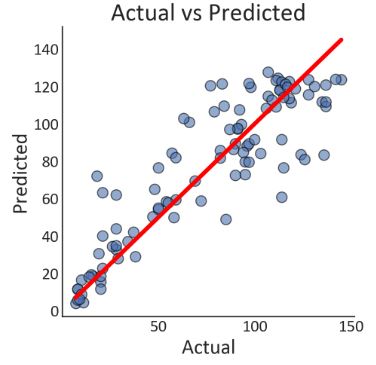
R-squared error: 78.13%
Root Mean Squared Error: 19.43
CPU times: total: 13.5 s
Wall time: 13.6 s
- Plotting the output of SVR test prediction
plt.style.use('seaborn-white')
plt.rcParams['figure.figsize']=5,5
plt.rcParams['font.family'] = 'Calibri'
plt.rcParams['lines.linewidth'] = 3
plt.rcParams['axes.labelsize']=20
plt.rcParams['xtick.labelsize']=16
plt.rcParams['ytick.labelsize']=16
plt.rcParams['legend.fontsize']=16

fig,ax = plt.subplots()
plt.title('Actual vs Predicted')
plt.xlabel('Actual')
plt.ylabel('Predicted')
g = sns.scatterplot(x=y_test,
                y=y_predictions,
                s=100,
                alpha=0.6,
                linewidth=1,
                edgecolor='black',
                ax=ax)
f = sns.lineplot(x=[min(y_test),max(y_test)],
             y=[min(y_test),max(y_test)],
             linewidth=4,
             color='red',
             ax=ax)

plt.annotate(text=('R-squared error: '+ "{:.2%}".format(model.score(X_test,y_test)) +'\n' +
                  'Root Mean Squared Error: '+ "{:.2f}".format(mean_squared_error(y_test,y_predictions,squared=False))),
             xy=(0,150),
             size='medium')

xlabels = ['{:,.0f}'.format(x) for x in g.get_xticks()]
g.set_xticklabels(xlabels)
ylabels = ['{:,.0f}'.format(x) for x in g.get_yticks()]
g.set_yticklabels(ylabels)
sns.despine()
plt.style.use('seaborn-white')
plt.rcParams['figure.figsize']=20,5
sns.set(font_scale=2)

fig,ax = plt.subplots()
plt.ylabel('RUL')
plt.xlabel('Engine nr')

g = sns.lineplot(x = np.arange(0,len(df_train['engine'].unique())),
                y=y_test,
                color='green',
                label = 'actual',
                ax=ax)

f = sns.lineplot(x = np.arange(0,len(df_train['engine'].unique())),
                y=y_predictions,
                color='red',
                label = 'predictions',
                ax=ax)
ax.legend()

- Training the RandomForestRegressor model
%%time
from sklearn.ensemble import RandomForestRegressor
start = time.time()
model = RandomForestRegressor(n_jobs=-1,
n_estimators=500,
min_samples_leaf=1,
max_features='sqrt',
).fit(X_train,y_train)
end_train = time.time()
y_predictions = model.predict(X_test) # These are the predictions from the test data.
end_predict = time.time()
model_performance.loc['Random Forest'] = [model.score(X_test,y_test),
mean_squared_error(y_test,y_predictions,squared=False),
end_train-start,
end_predict-end_train,
end_predict-start]
print('R-squared error: '+ "{:.2%}".format(model.score(X_test,y_test)))
print('Root Mean Squared Error: '+ "{:.2f}".format(mean_squared_error(y_test,y_predictions,squared=False)))
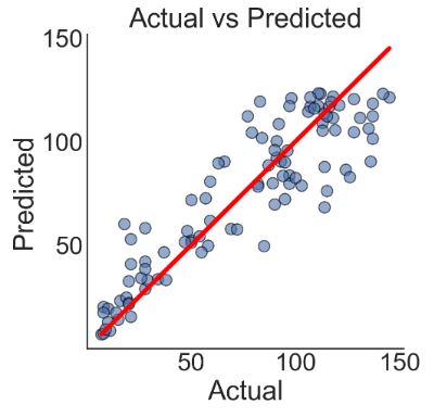
R-squared error: 81.09%
Root Mean Squared Error: 18.07
CPU times: total: 2min 15s
Wall time: 9.54 s
- Plotting the output of RandomForestRegressor test prediction
plt.style.use('seaborn-white')
plt.rcParams['figure.figsize']=5,5

fig,ax = plt.subplots()
plt.title('Actual vs Predicted')
plt.xlabel('Actual')
plt.ylabel('Predicted')
g = sns.scatterplot(x=y_test,
                y=y_predictions,
                s=100,
                alpha=0.6,
                linewidth=1,
                edgecolor='black',
                ax=ax)
f = sns.lineplot(x=[min(y_test),max(y_test)],
             y=[min(y_test),max(y_test)],
             linewidth=4,
             color='red',
             ax=ax)

plt.annotate(text=('R-squared error: '+ "{:.2%}".format(model.score(X_test,y_test)) +'\n' +
                  'Root Mean Squared Error: '+ "{:.2f}".format(mean_squared_error(y_test,y_predictions,squared=False))),
             xy=(0,150),
             size='medium')

xlabels = ['{:,.0f}'.format(x) for x in g.get_xticks()]
g.set_xticklabels(xlabels)
ylabels = ['{:,.0f}'.format(x) for x in g.get_yticks()]
g.set_yticklabels(ylabels)
sns.despine()
plt.style.use('seaborn-white')
plt.rcParams['figure.figsize']=20,5
sns.set(font_scale=2)
fig,ax = plt.subplots()
plt.ylabel('RUL')
plt.xlabel('Engine nr')

g = sns.lineplot(x = np.arange(0,len(df_train['engine'].unique())),
                y=y_test,
                color='green',
                label = 'actual',
                ax=ax)

f = sns.lineplot(x = np.arange(0,len(df_train['engine'].unique())),
                y=y_predictions,
                color='red',
                label = 'predictions',
                ax=ax)
ax.legend()

- Read more about the dataset and the implemented Python algorithm.
LSTM TensorFlow Keras
- Let’s discuss RUL prediction using LSTM TensorFlow Keras
- We begin with importing libraries, reading the input dataset train/test/RUL FD001, and performing exploratory data analysis (EDA)
import numpy as np
import pandas as pd
import os
import matplotlib.pyplot as plt
import seaborn as sns
from sklearn.ensemble import RandomForestRegressor
from sklearn.metrics import mean_absolute_error
from sklearn.metrics import r2_score
from sklearn.metrics import mean_squared_error
from sklearn.linear_model import LinearRegression
from sklearn.preprocessing import StandardScaler
from pylab import rcParams
import math
import xgboost
import time
from tqdm import tqdm
import keras.models
import keras.layers
from sklearn.model_selection import train_test_split
import tensorflow as tf
from tensorflow.keras.models import Sequential
from tensorflow.keras import layers
import warnings
warnings.simplefilter('ignore')

data_train = pd.read_csv("train_FD001.txt",sep=" ",header=None)
data_test = pd.read_csv("test_FD001.txt",sep=" ",header=None)
data_RUL = pd.read_csv("RUL_FD001.txt",sep=" ",header=None)

train_copy = data_train
test_copy = data_test

data_train.drop(columns=[26,27],inplace=True)
data_test.drop(columns=[26,27],inplace=True)
data_RUL.drop(columns=[1],inplace=True)

columns_train = ['unit_ID','cycles','setting_1','setting_2','setting_3','T2','T24','T30','T50','P2','P15','P30','Nf',
           'Nc','epr','Ps30','phi','NRf','NRc','BPR','farB','htBleed','Nf_dmd','PCNfR_dmd','W31','W32' ]
data_train.columns = columns_train
#data_train.describe().T
- Defining a function to calculate the remaining useful life (RUL)
def add_rul(g):
    # Calculate the RUL as the difference between the maximum cycle value and the cycle value for each row
    g['RUL'] = max(g['cycles']) - g['cycles']
    return g

# Apply the add_rul function to the training data grouped by the unit ID
train = data_train.groupby('unit_ID').apply(add_rul)
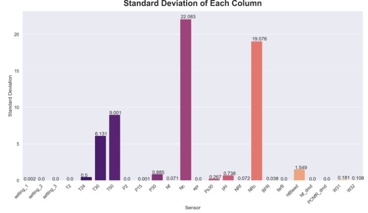
- Calculating STDEV of each column
plt.figure(figsize=(18, 9))
sns.set(font_scale=1.2)
subset_stats = data_train.agg(['mean', 'std']).T[2:]
ax = sns.barplot(x=subset_stats.index, y="std", data=subset_stats, palette='magma')
ax.set_xticklabels(ax.get_xticklabels(), rotation=45, ha="right")
ax.set_xlabel("Sensor")
ax.set_ylabel("Standard Deviation")
ax.set_title("Standard Deviation of Each Column", fontweight='bold', fontsize=24, pad=15)

for p in ax.patches:
    ax.annotate(str(round(p.get_height(),3)), (p.get_x() * 1.005, p.get_height() * 1.005))

plt.show()
- Let’s drop the unwanted columns
train.drop(columns=['Nf_dmd','PCNfR_dmd','P2','T2','setting_3','farB','epr'],inplace=True)
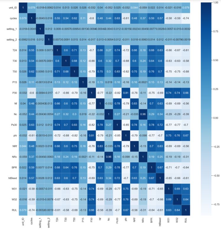
- Plotting the correlation heatmap
sns.heatmap(train.corr(),annot=True,cmap='Blues',linewidths=0.2)
fig=plt.gcf()
fig.set_size_inches(20,20)
plt.show()
- Preparing train/test data for LSTM
def process_targets(data_length, early_rul = None):
    if early_rul == None:
        return np.arange(data_length-1, -1, -1)
    else:
        early_rul_duration = data_length - early_rul
        if early_rul_duration <= 0:
            return np.arange(data_length-1, -1, -1)
        else:
            return np.append(early_rul*np.ones(shape = (early_rul_duration,)), np.arange(early_rul-1, -1, -1))

def process_input_data_with_targets(input_data, target_data = None, window_length = 1, shift = 1):
    num_batches = np.int(np.floor((len(input_data) - window_length)/shift)) + 1
    num_features = input_data.shape[1]
    output_data = np.repeat(np.nan, repeats = num_batches * window_length * num_features).reshape(num_batches, window_length,
                                                                                                  num_features)
    if target_data is None:
        for batch in range(num_batches):
            output_data[batch,:,:] = input_data[(0+shift*batch):(0+shift*batch+window_length),:]
        return output_data
    else:
        output_targets = np.repeat(np.nan, repeats = num_batches)
        for batch in range(num_batches):
            output_data[batch,:,:] = input_data[(0+shift*batch):(0+shift*batch+window_length),:]
            output_targets[batch] = target_data[(shift*batch + (window_length-1))]
        return output_data, output_targets

def process_test_data(test_data_for_an_engine, window_length, shift, num_test_windows = 1):

    max_num_test_batches = np.int(np.floor((len(test_data_for_an_engine) - window_length)/shift)) + 1
    if max_num_test_batches < num_test_windows:
        required_len = (max_num_test_batches -1)* shift + window_length
        batched_test_data_for_an_engine = process_input_data_with_targets(test_data_for_an_engine[-required_len:, :],
                                                                          target_data = None,
                                                                          window_length= window_length, shift = shift)
        return batched_test_data_for_an_engine, max_num_test_batches
    else:
        required_len = (num_test_windows - 1) * shift + window_length
        batched_test_data_for_an_engine = process_input_data_with_targets(test_data_for_an_engine[-required_len:, :],
                                                                          target_data = None,
                                                                          window_length= window_length, shift = shift)
        return batched_test_data_for_an_engine, num_test_windows

test_data = pd.read_csv("test_FD001.txt", sep = "\s+", header = None,names=columns_train )
true_rul = pd.read_csv("RUL_FD001.txt", sep = '\s+', header = None)

window_length = 30
shift = 1
early_rul = 125
processed_train_data = []
processed_train_targets = []
num_test_windows = 5
processed_test_data = []
num_test_windows_list = []

columns_to_be_dropped =['unit_ID','setting_1','setting_2','setting_3', 'T2', 'P2','P15','P30', 'epr',
                 'farB', 'Nf_dmd', 'PCNfR_dmd']

train_data_first_column = data_train ["unit_ID"]
test_data_first_column = test_data["unit_ID"]

scaler = StandardScaler()
train_data = scaler.fit_transform(data_train.drop(columns = columns_to_be_dropped))
test_data = scaler.transform(test_data.drop(columns = columns_to_be_dropped))

train_data = pd.DataFrame(data = np.c_[train_data_first_column, train_data])
test_data = pd.DataFrame(data = np.c_[test_data_first_column, test_data])

num_train_machines = len(train_data[0].unique())
num_test_machines = len(test_data[0].unique())

for i in np.arange(1, num_train_machines + 1):
    temp_train_data = train_data[train_data[0] == i].drop(columns = [0]).values

    # Determine whether it is possible to extract training data with the specified window length.
    if (len(temp_train_data) < window_length):
        print("Train engine {} doesn't have enough data for window_length of {}".format(i, window_length))
        raise AssertionError("Window length is larger than number of data points for some engines. "
                             "Try decreasing window length.")

    temp_train_targets = process_targets(data_length = temp_train_data.shape[0], early_rul = early_rul)
    data_for_a_machine, targets_for_a_machine = process_input_data_with_targets(temp_train_data, temp_train_targets,
                                                                                window_length= window_length, shift = shift)

    processed_train_data.append(data_for_a_machine)
    processed_train_targets.append(targets_for_a_machine)

processed_train_data = np.concatenate(processed_train_data)
processed_train_targets = np.concatenate(processed_train_targets)

for i in np.arange(1, num_test_machines + 1):
    temp_test_data = test_data[test_data[0] == i].drop(columns = [0]).values

    # Determine whether it is possible to extract test data with the specified window length.
    if (len(temp_test_data) < window_length):
        print("Test engine {} doesn't have enough data for window_length of {}".format(i, window_length))
        raise AssertionError("Window length is larger than number of data points for some engines. "
                             "Try decreasing window length.")

    # Prepare test data
    test_data_for_an_engine, num_windows = process_test_data(temp_test_data, window_length=window_length, shift = shift,
                                                             num_test_windows = num_test_windows)

    processed_test_data.append(test_data_for_an_engine)
    num_test_windows_list.append(num_windows)

processed_test_data = np.concatenate(processed_test_data)
true_rul = true_rul[0].values

# Shuffle training data
index = np.random.permutation(len(processed_train_targets))
processed_train_data, processed_train_targets = processed_train_data[index], processed_train_targets[index]
print("Processed training data shape: ", processed_train_data.shape)
print("Processed training RUL shape: ", processed_train_targets.shape)
print("Processed test data shape: ", processed_test_data.shape)
print("True RUL shape: ", true_rul.shape)

Processed training data shape:  (17731, 30, 14)
Processed training RUL shape:  (17731,)
Processed test data shape:  (497, 30, 14)
True RUL shape:  (100,)
- Training/validation data splitting with test_size = 0.2
processed_train_data, processed_val_data, processed_train_targets, processed_val_targets = train_test_split(processed_train_data,
                                                                                                            processed_train_targets,
                                                                                                            test_size = 0.2,
                                                                                                            random_state = 83)
print("Processed train data shape: ", processed_train_data.shape)
print("Processed validation data shape: ", processed_val_data.shape)
print("Processed train targets shape: ", processed_train_targets.shape)
print("Processed validation targets shape: ", processed_val_targets.shape)

Processed train data shape:  (14184, 30, 14)
Processed validation data shape:  (3547, 30, 14)
Processed train targets shape:  (14184,)
Processed validation targets shape:  (3547,)
- Training and validating the LSTM model
def create_compiled_model():
    model = Sequential([
        layers.LSTM(128, input_shape = (window_length, 14), return_sequences=True, activation = "tanh"),
        layers.LSTM(64, activation = "tanh", return_sequences = True),
        layers.LSTM(32, activation = "tanh"),
        layers.Dense(96, activation = "relu"),
        layers.Dense(128, activation = "relu"),
        layers.Dense(1)
    ])
    model.compile(loss = "mse", optimizer = tf.keras.optimizers.Adam(learning_rate=0.001))
    return model

def scheduler(epoch):
    if epoch < 5:
        return 0.001
    else:
        return 0.0001
callback = tf.keras.callbacks.LearningRateScheduler(scheduler, verbose = 1)
model = create_compiled_model()
history = model.fit(processed_train_data, processed_train_targets, epochs = 10,
                    validation_data = (processed_val_data, processed_val_targets),
                    callbacks = callback,
                    batch_size = 128, verbose = 2)

Epoch 1: LearningRateScheduler setting learning rate to 0.001.
Epoch 1/10
111/111 - 13s - loss: 3085.1455 - val_loss: 410.2751 - lr: 0.0010 - 13s/epoch - 119ms/step

Epoch 2: LearningRateScheduler setting learning rate to 0.001.
Epoch 2/10
111/111 - 10s - loss: 246.6438 - val_loss: 235.8336 - lr: 0.0010 - 10s/epoch - 90ms/step

Epoch 3: LearningRateScheduler setting learning rate to 0.001.
Epoch 3/10
111/111 - 11s - loss: 171.5130 - val_loss: 145.6538 - lr: 0.0010 - 11s/epoch - 95ms/step

Epoch 4: LearningRateScheduler setting learning rate to 0.001.
Epoch 4/10
111/111 - 12s - loss: 145.4168 - val_loss: 137.1005 - lr: 0.0010 - 12s/epoch - 111ms/step

Epoch 5: LearningRateScheduler setting learning rate to 0.001.
Epoch 5/10
111/111 - 13s - loss: 125.2865 - val_loss: 117.3468 - lr: 0.0010 - 13s/epoch - 113ms/step

Epoch 6: LearningRateScheduler setting learning rate to 0.0001.
Epoch 6/10
111/111 - 12s - loss: 101.7331 - val_loss: 100.6895 - lr: 1.0000e-04 - 12s/epoch - 111ms/step

Epoch 7: LearningRateScheduler setting learning rate to 0.0001.
Epoch 7/10
111/111 - 12s - loss: 97.5773 - val_loss: 97.9624 - lr: 1.0000e-04 - 12s/epoch - 110ms/step

Epoch 8: LearningRateScheduler setting learning rate to 0.0001.
Epoch 8/10
111/111 - 12s - loss: 95.0853 - val_loss: 95.2373 - lr: 1.0000e-04 - 12s/epoch - 107ms/step

Epoch 9: LearningRateScheduler setting learning rate to 0.0001.
Epoch 9/10
111/111 - 12s - loss: 92.5085 - val_loss: 93.2352 - lr: 1.0000e-04 - 12s/epoch - 112ms/step

Epoch 10: LearningRateScheduler setting learning rate to 0.0001.
Epoch 10/10
111/111 - 13s - loss: 89.6266 - val_loss: 95.0076 - lr: 1.0000e-04 - 13s/epoch - 115ms/step
- Computing RMSE and S-score
rul_pred = model.predict(processed_test_data).reshape(-1)
preds_for_each_engine = np.split(rul_pred, np.cumsum(num_test_windows_list)[:-1])
mean_pred_for_each_engine = [np.average(ruls_for_each_engine, weights = np.repeat(1/num_windows, num_windows))
                             for ruls_for_each_engine, num_windows in zip(preds_for_each_engine, num_test_windows_list)]
RMSE = np.sqrt(mean_squared_error(true_rul, mean_pred_for_each_engine))
print("RMSE: ", RMSE)
16/16 [==============================] - 1s 12ms/step
RMSE:  15.48950085023228

def compute_s_score(rul_true, rul_pred):
    diff = rul_pred - rul_true
    return np.sum(np.where(diff < 0, np.exp(-diff/13)-1, np.exp(diff/10)-1))
s_score = compute_s_score(true_rul, preds_for_last_example)
print("S-score: ", s_score)

S-score:  470.87409883085155
- Plotting RUL vs Engine Nr
plt.figure(figsize=(20, 5))
plt.plot(true_rul, label = "True RUL", color = "green")
plt.plot(preds_for_last_example, label = "Pred RUL", color = "red")
plt.rcParams.update({'font.size': 22})
plt.ylabel('RUL')
plt.xlabel('Engine nr')
plt.legend()
plt.show()

- Plotting train/test loss vs epoch
print(history.history.keys())
dict_keys(['loss', 'val_loss', 'lr'])

# summarize history for loss
plt.figure(figsize=(10, 6))
plt.rcParams.update({'font.size': 22})
plt.plot(history.history['loss'])
plt.plot(history.history['val_loss'])
plt.title('model loss')
plt.ylabel('loss')
plt.xlabel('epoch')
plt.legend(['train', 'test'], loc='upper left')
plt.show()

- Read more:
RUL prediction using LSTM for Aircraft Engine
Conclusions
- AI-powered prognostics and health management is an important topic in industry for predicting state of assets to avoid downtime and failures.
- In this study, we have used the Kaggle version of the public dataset for asset degradation modeling from NASA. The dataset consists of multiple multivariate time series. It includes Run-to-Failure simulated data from turbo fan jet engines.
- Each time series is from a different engine i.e., the data can be considered to be from a fleet of engines of the same type. Each engine starts with different degrees of initial wear and manufacturing variation which is unknown to the user. This wear and variation is considered normal, i.e., it is not considered a fault condition. There are three operational settings that have a substantial effect on engine performance. These settings are also included in the data. The data is contaminated with sensor noise.
- We have implemented statsmodels OLS, SciKit-Learn regression (viz. KNN, SVR, and Random Forest) and LSTM algorithms that predict the remaining useful life (RUL) of each engine in the test dataset. RUL is equivalent of number of flights remained for the engine after the last data point in the test dataset.
- Our main focus was on accurately recording low RUL values to prevent putting the engine at danger and forecasting the RUL of the turbofan engine while accounting for HPC failure.
- The high LSTM S-score of 470.87 indicates a good performance of the prediction model. This score is a measure of the difference between the actual and predicted RUL values normalized by the standard deviation of the RUL.
- The Random Forest regression of test data yields R-squared error of 81.09% and Root Mean Squared Error of 18.07. This model seems to be accurate and robust.
- We have done a thorough overview of the NASA turbofan regression problem and have provided detailed analysis of the dataset, feature selection, visualization and modeling considerations. Additionally, we highlighted our preferred ML/DL models.
- Our next step is to deploy the final Python code as a streamlit web app that provides an interactive GUI for maintenance teams to input engine data and generate accurate predictions of engine failures.
Explore More
- Responsible AI in Predictive Maintenance — Using NASA Turbofan Engine Degradation Dataset — Using sklearn
- Predictive Maintenance of NASA Turbofan Engines Using Traditional and Ensemble Machine Learning Techniques
- Machine Learning-Based Predictive Analytics for Aircraft Engine Conceptual Design
- LSTM for predictive maintenance of turbofan engines

Leave a comment