
- Recently, Time Series Forecasting (TSF) has gained a lot of attention as the go-to strategy across various industry sectors (sales, stock prices, meteorology, energy consumption, marketing, etc.). TSF is used to forecast trends, seasonality, and other patterns in time series data.
- In this post, we will compare several popular TSF methods in terms of their forecasting performance on a set of 4 real-world time series: Air Passengers, the U.S. Wholesale Price Index (WPI), BTC-USD price, and the Peyton Manning. Our evaluation will involve assessing the quality of the TSF and determining whether it is accurate and reliable. This may involve comparing the forecast to the actual values and using statistical performance measures, such as MAE, MAPE and RMSE, to evaluate its performance.
- Some advanced TSF models are ThymeBoost, Prophet, and AutoARIMA (pmdarima). These methods are based on historical data and build statistical models to identify patterns and trends in the data.
- In fact, several studies have shown that ThymeBoost outperforms traditional TSF models: Tyler Blume recently explored the ThymeBoost framework and compared its auto-forecasting performance to some of its peers.
- ThymeBoost is based on machine learning (ML) algorithms, including gradient boosting (GB) and deep learning. It combines time series decomposition with ML/GB to provide a balanced mix-and-match forecasting.
- At the most granular level are the trend, seasonal, and endogenous models. The key features of ThymeBoost include automation, multiple modeling options, performance evaluation, and tuning.
- Continue reading about the aforementioned TSF models and related feature engineering methods.
Table of Contents
Air Passengers
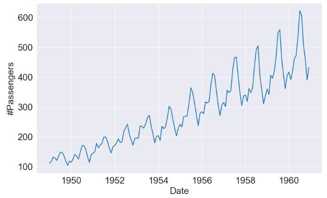
- Let’s begin with the most popular Airline Passenger dataset.
- Setting the working directory YOURPATH, importing the key libraries, and reading the input data
import os
os.chdir('YOURPATH')
os. getcwd()

!pip install ThymeBoost --upgrade

import numpy as np
import pandas as pd
from matplotlib import pyplot as plt
from ThymeBoost import ThymeBoost as tb
import seaborn as sns
sns.set_style("darkgrid")
plt.rcParams.update({'font.size': 18})
plt.figure(figsize=(10,6))
df = pd.read_csv('AirPassengers.csv')
df.index = pd.to_datetime(df['Month'])
y = df['#Passengers']
plt.xlabel('Date')
plt.ylabel('#Passengers')
plt.plot(y)
plt.show()
- Train/test data splitting as 70:30%
test_len = int(len(y) * 0.3)
al_train, al_test = y.iloc[:-test_len], y.iloc[-test_len:]
- Fitting a simple AutoARIMA model
import pmdarima as pm
arima = pm.auto_arima(al_train,
                      seasonal=True,
                      m=12,
                      trace=True,
                      error_action='warn',
                      n_fits=50)
pmd_predictions = arima.predict(n_periods=len(al_test))
arima_mae = np.mean(np.abs(al_test - pmd_predictions))
arima_rmse = (np.mean((al_test - pmd_predictions)**2))**.5
arima_mape = np.sum(np.abs(pmd_predictions - al_test)) / (np.sum((np.abs(al_test))))
Performing stepwise search to minimize aic
 ARIMA(2,1,2)(1,1,1)[12]             : AIC=654.029, Time=0.47 sec
 ARIMA(0,1,0)(0,1,0)[12]             : AIC=657.288, Time=0.01 sec
 ARIMA(1,1,0)(1,1,0)[12]             : AIC=650.553, Time=0.06 sec
 ARIMA(0,1,1)(0,1,1)[12]             : AIC=651.123, Time=0.12 sec
 ARIMA(1,1,0)(0,1,0)[12]             : AIC=652.376, Time=0.02 sec
 ARIMA(1,1,0)(2,1,0)[12]             : AIC=652.523, Time=0.18 sec
 ARIMA(1,1,0)(1,1,1)[12]             : AIC=652.538, Time=0.13 sec
 ARIMA(1,1,0)(0,1,1)[12]             : AIC=650.954, Time=0.10 sec
 ARIMA(1,1,0)(2,1,1)[12]             : AIC=inf, Time=1.26 sec
 ARIMA(0,1,0)(1,1,0)[12]             : AIC=653.919, Time=0.06 sec
 ARIMA(2,1,0)(1,1,0)[12]             : AIC=652.418, Time=0.10 sec
 ARIMA(1,1,1)(1,1,0)[12]             : AIC=651.963, Time=0.11 sec
 ARIMA(0,1,1)(1,1,0)[12]             : AIC=650.738, Time=0.07 sec
 ARIMA(2,1,1)(1,1,0)[12]             : AIC=653.897, Time=0.16 sec
 ARIMA(1,1,0)(1,1,0)[12] intercept   : AIC=652.271, Time=0.17 sec

Best model:  ARIMA(1,1,0)(1,1,0)[12]
Total fit time: 3.060 seconds
print (arima_mae)
print (arima_rmse)
print (arima_mape)

2.3930597256495694
2.8132108675986482
0.022076196808772784
- Fitting the multiplicative Prophet model
from prophet import Prophet
prophet_train_df = al_train.reset_index()
prophet_train_df.columns = ['ds', 'y']
prophet = Prophet(seasonality_mode='multiplicative')
prophet.fit(prophet_train_df)
future_df = prophet.make_future_dataframe(periods=len(al_test), freq='M')
prophet_forecast = prophet.predict(future_df)
prophet_predictions = prophet_forecast['yhat'].iloc[-len(al_test):]
prophet_mae = np.mean(np.abs(al_test - prophet_predictions.values))
prophet_rmse = (np.mean((al_test - prophet_predictions.values)**2))**.5
prophet_mape = np.sum(np.abs(prophet_predictions.values - al_test)) / (np.sum((np.abs(al_test))))
print (prophet_mae)
print (prophet_rmse)
print (prophet_mape)

8.315019543856259
9.230116817444786
0.07670682263023607
- Fitting the ThymeBoost model
boosted_model = tb.ThymeBoost(verbose=0)
output = boosted_model.autofit(al_train,
                               seasonal_period=12)
predicted_output = boosted_model.predict(output, len(al_test))
tb_mae = np.mean(np.abs(al_test - predicted_output['predictions']))
tb_rmse = (np.mean((al_test - predicted_output['predictions'])**2))**.5
tb_mape = np.sum(np.abs(predicted_output['predictions'] - al_test)) / (np.sum((np.abs(al_test))))

Optimal model configuration: {'trend_estimator': ['linear', 'ses'], 'fit_type': 'global', 'seasonal_period': [12], 'arima_order': None, 'seasonal_estimator': 'fourier', 'global_cost': 'mse', 'additive': False, 'seasonality_weights': array([ 2,  2,  2,  2,  2,  2,  2,  2,  2,  2,  2,  2,  3,  3,  3,  3,  3,
        3,  3,  3,  3,  3,  3,  3,  4,  4,  4,  4,  4,  4,  4,  4,  4,  4,
        4,  4,  5,  5,  5,  5,  5,  5,  5,  5,  5,  5,  5,  5,  6,  6,  6,
        6,  6,  6,  6,  6,  6,  6,  6,  6,  7,  7,  7,  7,  7,  7,  7,  7,
        7,  7,  7,  7,  8,  8,  8,  8,  8,  8,  8,  8,  8,  8,  8,  8,  9,
        9,  9,  9,  9,  9,  9,  9,  9,  9,  9,  9, 10, 10, 10, 10, 10]), 'exogenous': None}
Params ensembled: False
print (tb_mae)
print (tb_rmse)
print (tb_mape)

44.2778947853649
50.34661221952847
0.10477379901885817
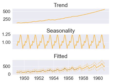
- Plotting model components
plt.rcParams.update({'font.size': 18})
plt.figure(figsize=(10,15))
boosted_model.plot_components(output, predicted_output)
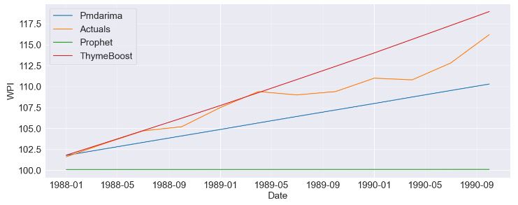
- Plotting actuals, pmdarima, prophet, and ThymeBoost (TB) for the test data
plt.rcParams.update({'font.size': 18})
plt.figure(figsize=(10,6))
plt.plot(pmd_predictions, label='Pmdarima')
plt.plot(pmd_predictions.index,al_test.values, label='Actuals')
plt.plot(pmd_predictions.index,prophet_predictions.values, label='Prophet')
plt.plot(pmd_predictions.index,predicted_output['predictions'].values, label='ThymeBoost')
plt.xlabel('Date')
plt.ylabel('#Passengers')
plt.legend()
plt.show()

U.S. WPI
- The 2nd dataset is the U.S. Wholesale Price Index (WPI) from 1960 to 1990 and the example is taken from the aforementioned article.
from  statsmodels.datasets import webuse
plt.rcParams.update({'font.size': 18})
plt.figure(figsize=(10,6))
dta = webuse('wpi1')
ts_wpi = dta['wpi']
ts_wpi.index = pd.to_datetime(dta['t'])
test_len = int(len(ts_wpi) * 0.1)
ts_wpi = ts_wpi.astype(float)
wpi_train, wpi_test = ts_wpi.iloc[:-test_len], ts_wpi.iloc[-test_len:]
plt.xlabel('Date')
plt.ylabel('WPI')
plt.plot(ts_wpi)
plt.show()

- Fitting the AutoARIMA model
import pmdarima as pm
# Fit a simple auto_arima model
arima = pm.auto_arima(wpi_train,
                      seasonal=False,
                      trace=True,
                      error_action='warn',
                      n_fits=50)
pmd_predictions = arima.predict(n_periods=len(wpi_test))
arima_mae = np.mean(np.abs(wpi_test - pmd_predictions))
arima_rmse = (np.mean((wpi_test - pmd_predictions)**2))**.5
arima_mape = np.sum(np.abs(pmd_predictions - wpi_test)) / (np.sum((np.abs(wpi_test))))

Performing stepwise search to minimize aic
 ARIMA(2,2,2)(0,0,0)[0] intercept   : AIC=233.402, Time=0.24 sec
 ARIMA(0,2,0)(0,0,0)[0] intercept   : AIC=245.760, Time=0.02 sec
 ARIMA(1,2,0)(0,0,0)[0] intercept   : AIC=233.922, Time=0.02 sec
 ARIMA(0,2,1)(0,0,0)[0] intercept   : AIC=229.373, Time=0.04 sec
 ARIMA(0,2,0)(0,0,0)[0]             : AIC=243.762, Time=0.01 sec
 ARIMA(1,2,1)(0,0,0)[0] intercept   : AIC=230.888, Time=0.04 sec
 ARIMA(0,2,2)(0,0,0)[0] intercept   : AIC=230.976, Time=0.04 sec
 ARIMA(1,2,2)(0,0,0)[0] intercept   : AIC=inf, Time=0.19 sec
 ARIMA(0,2,1)(0,0,0)[0]             : AIC=227.412, Time=0.02 sec
 ARIMA(1,2,1)(0,0,0)[0]             : AIC=228.930, Time=0.03 sec
 ARIMA(0,2,2)(0,0,0)[0]             : AIC=229.018, Time=0.03 sec
 ARIMA(1,2,0)(0,0,0)[0]             : AIC=231.935, Time=0.01 sec
 ARIMA(1,2,2)(0,0,0)[0]             : AIC=inf, Time=0.14 sec

Best model:  ARIMA(0,2,1)(0,0,0)[0]
Total fit time: 0.860 seconds
print (arima_mae)
print (arima_rmse)
print (arima_mape)

2.3930597256495694
2.8132108675986482
0.022076196808772784
- Fitting the Prophet model
from prophet import Prophet
prophet_train_df = wpi_train.reset_index()
prophet_train_df.columns = ['ds', 'y']
prophet = Prophet(yearly_seasonality=False)
prophet.fit(prophet_train_df)
future_df = prophet.make_future_dataframe(periods=len(wpi_test))
prophet_forecast = prophet.predict(future_df)
prophet_predictions = prophet_forecast['yhat'].iloc[-len(wpi_test):]
prophet_mae = np.mean(np.abs(wpi_test - prophet_predictions.values))
prophet_rmse = (np.mean((wpi_test - prophet_predictions.values)**2))**.5
prophet_mape = np.sum(np.abs(prophet_predictions.values - wpi_test)) / (np.sum((np.abs(wpi_test))))

print (prophet_mae)
print (prophet_rmse)
print (prophet_mape)

8.315019543856259
9.230116817444786
0.07670682263023607
- Fitting the ThymeBoost model
boosted_model = tb.ThymeBoost(verbose=0)
output = boosted_model.autofit(wpi_train,
                               seasonal_period=0)

predicted_output = boosted_model.predict(output, forecast_horizon=len(wpi_test))
tb_mae = np.mean(np.abs((wpi_test.values) - predicted_output['predictions']))
tb_rmse = (np.mean((wpi_test.values - predicted_output['predictions'].values)**2))**.5
tb_mape = np.sum(np.abs(predicted_output['predictions'].values - wpi_test.values)) / (np.sum((np.abs(wpi_test.values))))

Optimal model configuration: {'trend_estimator': ['linear', 'ses'], 'fit_type': 'global', 'seasonal_period': 0, 'arima_order': None, 'seasonal_estimator': 'fourier', 'global_cost': 'mse', 'additive': False, 'exogenous': None}
Params ensembled: False

print(boosted_model.optimized_params)

{'trend_estimator': ['linear', 'ses'], 'fit_type': 'global', 'seasonal_period': 0, 'arima_order': None, 'seasonal_estimator': 'fourier', 'global_cost': 'mse', 'additive': False, 'exogenous': None}

print (tb_mae)
print (tb_rmse)
print (tb_mape)

1.8009677718849417
2.4801489070703315
0.0166140938950435
- Comparing the TSF results vs actuals
plt.rcParams.update({'font.size': 18})
plt.figure(figsize=(16,6))
plt.plot(pmd_predictions.index,pmd_predictions, label='Pmdarima')
plt.plot(pmd_predictions.index,wpi_test.values, label='Actuals')
plt.plot(pmd_predictions.index,prophet_predictions.values, label='Prophet')
plt.plot(pmd_predictions.index,predicted_output['predictions'].values, label='ThymeBoost')
plt.xlabel('Date')
plt.ylabel('WPI')
plt.legend()
plt.show()
BTC-USD
- Let’s look at the BTC-USD TSF by modifying the ThymeBoost code with various QC options
from ThymeBoost import ThymeBoost as tb
import seaborn as sns
sns.set_style('darkgrid')
import yfinance as yf
msft = yf.Ticker("BTC-USD")

# get historical market data
hist = msft.history(period="max")

current_df = hist.iloc[-900:-50].reset_index()
future_df = hist.iloc[-50:].reset_index()

y_train = current_df['High']
X_train = current_df[['Volume', 'Stock Splits']]

y_test = future_df['High']
X_test = future_df[['Volume', 'Stock Splits']]
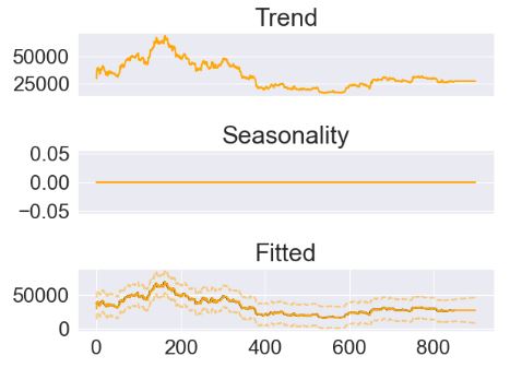
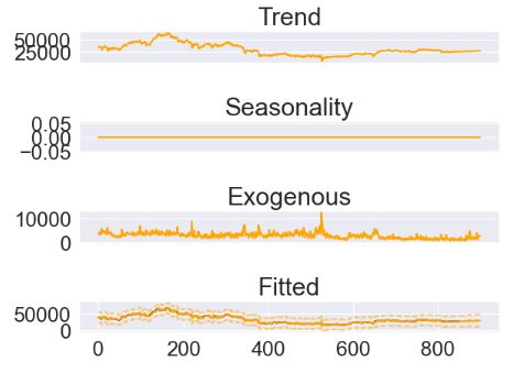
- Fitting the ThymeBoost model with the ARIMA trend
boosted_model = tb.ThymeBoost(verbose=0)
output = boosted_model.fit(y_train,
                           trend_estimator='arima',
                           arima_order=(2,1,2),
                           global_cost='mse',
                           fit_type='global',
                           )
predicted_output = boosted_model.predict(output, 50)
plt.rcParams.update({'font.size': 18})
plt.figure(figsize=(16,6))
boosted_model.plot_results(output, predicted_output)

plt.rcParams.update({'font.size': 18})
boosted_model.plot_components(output, predicted_output)
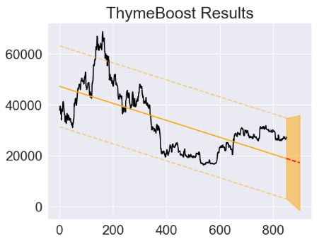
- Fitting the ThymeBoost model with the Linear + ARIMA trend
boosted_model = tb.ThymeBoost(verbose=0)
output = boosted_model.fit(y_train,
                           trend_estimator=['linear', 'arima'],
                           arima_order=(2,1,2),
                           global_cost='mse',
                           fit_type='global',
                           )
predicted_output = boosted_model.predict(output, 50)
plt.rcParams.update({'font.size': 18})
boosted_model.plot_results(output, predicted_output)
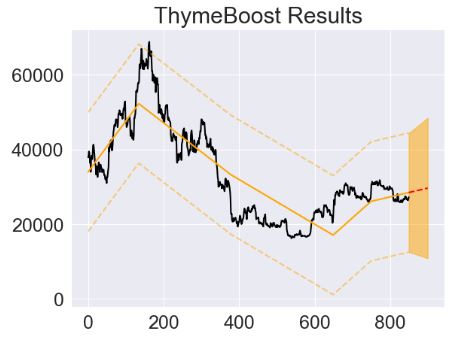
- Fitting the ThymeBoost model with the Linear + ARIMA trend and arima_order=’auto’
boosted_model = tb.ThymeBoost(verbose=1)
output = boosted_model.fit(y_train,
                           trend_estimator=['linear', 'arima'],
                           arima_order='auto',
                           global_cost='mse',
                           fit_type='global',
                           )
predicted_output = boosted_model.predict(output, 50)

********** Round 1 **********
Using Split: None
Fitting initial trend globally with trend model:
median()
seasonal model:
None
cost: 165160095.1694897
********** Round 2 **********
Using Split: None
Fitting global with trend model:
linear((1, None))
seasonal model:
None
cost: 86426761.83257383
********** Round 3 **********
Using Split: None
Fitting global with trend model:
arima(auto)
seasonal model:
None
cost: 1080981.535484013
==============================
Boosting Terminated
Using round 3
plt.rcParams.update({'font.size': 18})
boosted_model.plot_results(output, predicted_output)

- Revisiting the ThymeBoost model optimization based on the Exogeneous example code
from ThymeBoost import ThymeBoost as tb
import yfinance as yf
msft = yf.Ticker("BTC-USD")

# get historical market data
hist = msft.history(period="max")

current_df = hist.iloc[-900:-50].reset_index()
future_df = hist.iloc[-50:].reset_index()

y_train = current_df['High']
X_train = current_df[['Volume', 'Stock Splits']]

y_test = future_df['High']
X_test = future_df[['Volume', 'Stock Splits']]

boosted_model = tb.ThymeBoost(verbose=0)
output = boosted_model.fit(y_train,
                           trend_estimator=['linear','ses'],
                           seasonal_estimator='fourier',
                           global_cost='mse',
                           exogenous_estimator='ols',
                           fit_type=['local', 'global'],
                            exogenous=X_train,
                           )
predicted_output = boosted_model.predict(output, 50, future_exogenous=X_test)

plt.rcParams.update({'font.size': 18})
boosted_model.plot_results(output, predicted_output)

plt.rcParams.update({'font.size': 18})
boosted_model.plot_components(output, predicted_output)
- Fitting the ThymeBoost exogeneous model with rolling optimization
boosted_model = tb.ThymeBoost(verbose=0)
output = boosted_model.optimize(y_train,
                                trend_estimator=[['linear','ses'], 'linear'],
                                seasonal_estimator=['fourier'],
                                global_cost=['mse'],
                                exogenous_estimator=['ols', 'decision_tree'],
                                fit_type=[['local', 'global'], 'global'],
                                exogenous=[X_train, None],
                                optimization_strategy='rolling',
                                lag=32,
                                optimization_steps=8
                                )
Optimal model configuration: {'trend_estimator': ['linear', 'ses'], 'fit_type': ['local', 'global'], 'seasonal_period': None, 'seasonal_estimator': 'fourier', 'global_cost': 'mse', 'exogenous_estimator': 'ols', 'exogenous':           Volume  Stock Splits
0    34639423297             0
1    33070867190             0
2    35460750427             0
3    41831090187             0
4    35959473399             0
..           ...           ...
845   8192867686             0
846  11997833257             0
847   9985498161             0
848  11718380997             0
849  14079002707             0

[850 rows x 2 columns]}
Params ensembled: False
plt.rcParams.update({'font.size': 18})
boosted_model.plot_optimization(output)

predicted_output = boosted_model.predict(output, 50, future_exogenous=X_test)
plt.rcParams.update({'font.size': 18})
boosted_model.plot_results(output, predicted_output)

- Let’s optimize the ThymeBoost TSF using both linear and polynomial trends with multiple change points (cf. code)
from ThymeBoost import ThymeBoost as tb
import seaborn as sns
sns.set_style('darkgrid')
import yfinance as yf
msft = yf.Ticker("BTC-USD")

# get historical market data
hist = msft.history(period="max")

current_df = hist.iloc[-900:-50].reset_index()
future_df = hist.iloc[-50:].reset_index()

y_train = current_df['High']
X_train = current_df[['Volume', 'Stock Splits']]

y_test = future_df['High']
X_test = future_df[['Volume', 'Stock Splits']]

boosted_model = tb.ThymeBoost(verbose=0)
output = boosted_model.fit(y_train,
                           trend_estimator='linear',
                           global_cost='mse',
                           fit_type='global',
                           )
predicted_output = boosted_model.predict(output, 50)

plt.rcParams.update({'font.size': 18})
boosted_model.plot_results(output, predicted_output)
- Fitting the ThymeBoost model using the global parabolic regression
boosted_model = tb.ThymeBoost(verbose=0)
output = boosted_model.fit(y_train,
                           trend_estimator='linear',
                           poly=2,
                           global_cost='mse',
                           fit_type='global',
                           )
predicted_output = boosted_model.predict(output, 50)

plt.rcParams.update({'font.size': 18})
boosted_model.plot_results(output, predicted_output)

- Fitting the ThymeBoost model using the local 3rd order polynomial regression
boosted_model = tb.ThymeBoost(verbose=0)
output = boosted_model.fit(y_train,
                           trend_estimator='linear',
                           poly=3,
                           global_cost='mse',
                           fit_type='local',
                           )
predicted_output = boosted_model.predict(output, 50)

plt.rcParams.update({'font.size': 18})
boosted_model.plot_results(output, predicted_output)

- Fitting the ThymeBoost model using the local 2rd order polynomial regression
boosted_model = tb.ThymeBoost(verbose=0)
output = boosted_model.fit(y_train,
                           trend_estimator='linear',
                           poly=2,
                           global_cost='maicc',
                           fit_type='local',
                           )
predicted_output = boosted_model.predict(output, 50)

plt.rcParams.update({'font.size': 18})
boosted_model.plot_results(output, predicted_output)

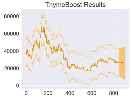
- Fitting the ThymeBoost model using the local linear regression with split_strategy=’gradient’
boosted_model = tb.ThymeBoost(verbose=0,
                             approximate_splits=True,
                              n_split_proposals=50,
                             split_strategy='gradient')
output = boosted_model.fit(y_train,
                           trend_estimator='linear',
                           poly=1,
                           global_cost='maicc',
                           fit_type='local',
                           )
predicted_output = boosted_model.predict(output, 50)

plt.rcParams.update({'font.size': 18})
boosted_model.plot_results(output, predicted_output)
- Fitting the ThymeBoost model using the local linear regression with approximate_splits=False
boosted_model = tb.ThymeBoost(verbose=0,
                             approximate_splits=False)
output = boosted_model.fit(y_train,
                           trend_estimator='linear',
                           poly=1,
                           global_cost='maicc',
                           fit_type='local',
                           )
predicted_output = boosted_model.predict(output, 50)

plt.rcParams.update({'font.size': 18})
boosted_model.plot_results(output, predicted_output)
Peyton Manning
import pandas as pd
import matplotlib.pyplot as plt
from prophet import Prophet
import numpy as np
import seaborn as sns
sns.set_style('darkgrid')
df = pd.read_csv('https://raw.githubusercontent.com/facebook/prophet/main/examples/example_wp_log_peyton_manning.csv')
plt.rcParams.update({'font.size': 14})
plt.figure(figsize=(14,10))
m = Prophet(weekly_seasonality=True)
m.fit(df)
future = m.make_future_dataframe(periods=2 * 365)
forecast = m.predict(future)
m.plot(forecast)
m.plot_components(forecast)
plt.show()


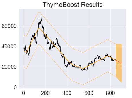
- Fitting the ThymeBoost model with 25 change points and trend_estimator=[‘lbf’]
from ThymeBoost import ThymeBoost as tb
boosted_model = tb.ThymeBoost(verbose=1,
                            n_rounds=None)

output = boosted_model.fit(df['y'].values,
                            seasonal_period=[365],
                            trend_estimator=['lbf'],
                            n_changepoints=25
                            )

predicted_output = boosted_model.predict(output,
                                          365 * 2)
********** Round 1 **********
Using Split: None
Fitting initial trend globally with trend model:
median()
seasonal model:
fourier(10, False)
cost: -2341.8470210049586
********** Round 2 **********
Using Split: None
Fitting global with trend model:
lbf(25)
seasonal model:
fourier(10, False)
cost: -3283.6285756724137
==============================
Boosting Terminated
Using round 2
plt.rcParams.update({'font.size': 14})
plt.figure(figsize=(14,10))
boosted_model.plot_results(output, predicted_output)
boosted_model.plot_components(output, predicted_output)
![Fitting the ThymeBoost model with 25 change points and trend_estimator=['lbf']](https://newdigitals.org/wp-content/uploads/2023/11/tb_forecast.jpg?w=481)
- Comparing trends predicted by Prophet and ThymeBoost
plt.rcParams.update({'font.size': 14})
plt.figure(figsize=(10,6))
plt.plot(np.append(output['trend'].values, predicted_output['predicted_trend'].values), label='ThymeBoost')
plt.plot(forecast['trend'], label='Prophet')
plt.legend()
plt.show()

- Comparing yearly seasonality predicted by ThymeBoost and Prophet
plt.rcParams.update({'font.size': 14})
plt.figure(figsize=(10,6))
plt.plot(np.append(output['seasonality'].values, predicted_output['predicted_seasonality'].values), label='ThymeBoost', alpha=.5)
plt.plot(forecast['additive_terms'], label='Prophet', alpha=.5)
plt.legend()
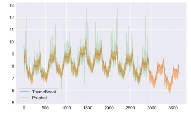
- Comparing time series predicted by ThymeBoost and Prophet
plt.rcParams.update({'font.size': 14})
plt.figure(figsize=(10,6))
plt.plot(np.append(output['yhat'].values, predicted_output['predictions'].values), label='ThymeBoost', alpha=.5)
plt.plot(forecast['yhat'], label='Prophet', alpha=.5)
plt.plot(df['y'].values, alpha=.2)
plt.legend()
Summary
- This study evaluates AutoARIMA, Facebook Prophet and ThymeBoost in terms of their forecasting performance on a set of 4 real-world time series: Air Passengers, the U.S. Wholesale Price Index (WPI), BTC-USD price, and the Peyton Manning.
- ThymeBoost is a Python library typically used in ML/AI applications. It combines the traditional decomposition process with gradient boosting to provide a flexible mix-and-match time series framework for trend/seasonality/endogenous decomposition and TSF. ThymeBoost supports a range of different modeling techniques, including gradient boosting, deep learning, and classical statistical models, allowing users to choose the most appropriate method for their data and forecasting needs.
- Prophet is a TSF library that can handle missing data, seasonality, and trends in the data. The TSF model can be tuned by adjusting trends, seasonality, and holidays.
- An ARIMA (autoregressive integrated moving average) model is a type of statistical model that is used to analyze and forecast time series data. It is a combination of three different models: an autoregressive (AR) model, an integrated (I) model, and a moving average (MA) model. The AR component models the relationship between the current and past values of the time series data. The I component models the data difference in order to satisfy the condition of stationarity. The MA models the remaining noise.
- Our next study will evaluate other statistical models such as TSMixer, DARTS (Detection of Anomalies in Time Series), Tsfresh, Ruptures, and LSTM.
Explore More
- Python Quant Trading Challenge: Can Dividend Stocks, NG and BTC Diversify Positively Correlated Big Tech Assets?
- Robust Anomaly Detection using the Isolation Forest Algorithm: Financial Transactions vs NYC Taxi Rides
- Time Series Forecasting of Hourly U.S.A. Energy Consumption – PJM East Electricity Grid
- Predicting the JPM Stock Price and Breakouts with Auto ARIMA, FFT, LSTM and Technical Trading Indicators
- SARIMAX X-Validation of EIA Crude Oil Prices Forecast in 2023 – 2. Brent
- Stock Forecasting with FBProphet


One-Time
Monthly
Yearly
Make a one-time donation
Make a monthly donation
Make a yearly donation
Choose an amount
€5.00
€15.00
€100.00
€5.00
€15.00
€100.00
€5.00
€15.00
€100.00
Or enter a custom amount
€
Your contribution is appreciated.
Your contribution is appreciated.
Your contribution is appreciated.
DonateDonate monthlyDonate yearly
Leave a comment