
SEO Title: Can Dividends, Natural Gas and Crypto Diversify Big Techs?
- The objective of this project is to implement several basic Quant Trading (QT) optimization ideas by analyzing tech growth, dividend stocks and highly volatile assets (commodities and crypto) in terms of risk/return optimization scenarios and (potential) diversification options.
- We will use the financial APIs to download real-time price charts of both individual stocks and stock portfolios.
- Several steps will be undertaken to validate the performance and reliability of our QT algorithms on historical data before going live with them in algorithmic trading.
- Project Scope and Specific Goals:
- Portfolio Optimization Scenario 1: MO + (AAPL, META, AMZN)
- Portfolio Optimization Scenario 2: (DIS, AMD) + (AAPL, TSLA)
- Portfolio 3: (a) [‘TATAMOTORS’,’DABUR’, ‘ICICIBANK’,’WIPRO’,’INFY’] and (b) [‘AXISBANK’, ‘HDFCBANK’, ‘ICICIBANK’, ‘KOTAKBANK’, ‘SBIN’] (Indian Stocks)
- In-Depth QT Analysis of Tech Growth Stocks: AAPL, META, and NVDA
- Backtesting of S&P 500 historical prices in terms of price anomalies
- Feasibility of short-term price prediction of the most volatile assets: commodities such as Natural Gas (NG) and crypto (BTC-USD).
Ultimately, we need to answer the following fundamental question: Can Dividend Kings, NGUSD and BTC-USD Diversify Growth Tech assets?
- Why Dividend Stocks:
Dividends are very popular among investors, especially those who want a steady stream of income from their investments. Some companies choose to share their profits with shareholders. These distributions are called dividends. First, they provide investors with regular income monthly, quarterly, or annually. Secondly, they offer a sense of safety. Stock prices are subject to volatility—whether that’s company-specific or industry-specific news or factors that affect the overall economy—so investors want to be sure they have some stability as well. Many companies that pay dividends already have an established track record of profits and profit-sharing.
- Why NGUSD:
Commodities are an alternative asset class that can provide a hedge against inflation and diversification away from the more mainstream asset classes.
Natural gas (NG) is one of the most traded commodities. NG prices have soared in 2022, reaching price levels not seen since 2008. From heating homes to powering industrial facilities, NG is a mainstay of the global energy mix. As the cleanest-burning fossil fuel, it’s a critical bridge fuel in the energy transition to lower-carbon alternatives. Read more here.
Alex Campbell, head of communications at Freetrade, comments: “Rather than backing some of these high-flying green energy companies that are still yet to ship a tried-and-tested product, companies in the natural gas supply sector tend to target efficient and hopefully predictable capital returns to shareholders through buybacks and dividends.”
Looking at demand and supply, the US is by far the largest consumer and exporter of NG.
- Is crypto mining a good idea?
While the cryptocurrency market appears to be more resilient now than it has been in the past, it’s still an extremely volatile, high risk and complex investment.
However, the stock correlation analysis indicates that BTC correlations with other assets are less than 0.2. In addition, most of its correlations with other assets are negative. This makes it ideal for inclusion in a portfolio to add diversification.
Table of Contents
- Portfolio 1: MO + (AAPL, META, AMZN)
- Portfolio 2: (DIS, AMD) + (AAPL, TSLA)
- AAPL Price LSTM Forecasting
- NVDA Entry/Exit Trading Signals
- NVDA Fundamental Analysis
- Indian Dividend Stock Portfolio 3
- BTC-USD Price Analysis and Forecasting
- Natural Gas Price Forecasting
- META Stock Isolation Forest Anomalies
- S&P 500 Historical Price Anomalies
- Summary
- References
- Explore More
- Prerequisites: Python, Jupyter with Anaconda IDE, Pandas, Numpy, Seaborn, Matplotlib, yfinance, pypfopt, OS, requests, Quantstats, sklearn, Plotly, and TensorFlow.
Portfolio 1: MO + (AAPL, META, AMZN)
- In this section, we will examine Portfolio 1 by implementing the stock market analysis and LSTM prediction pipeline.
- The stocks of interest are MO + (AAPL, META, AMZN).
- Why MO? Altria’s dividend yield is a huge 9.37%; the company’s main product has a loyal customer base; Altria walks a fine line between price and demand.
- Let’s set the working directory YOURPATH
import os
os.chdir('YOURPATH')
os. getcwd()
- Importing the key libraries and downloading stock prices
import pandas as pd
import numpy as np

import matplotlib.pyplot as plt
import seaborn as sns
sns.set_style('whitegrid')
plt.style.use("fivethirtyeight")
%matplotlib inline

# For reading stock data from yahoo
from pandas_datareader.data import DataReader
import yfinance as yf
from pandas_datareader import data as pdr

yf.pdr_override()

# For time stamps
from datetime import datetime


# The stocks we'll use for this analysis
tech_list = ['AAPL', 'META', 'MO', 'AMZN']

# Set up End and Start times for data grab

end = datetime.now()
start = datetime(end.year - 1, end.month, end.day)

for stock in tech_list:
    globals()[stock] = yf.download(stock, start, end)


company_list = [AAPL, META, MO, AMZN]
company_name = ["APPLE", "META", "ALTRIA", "AMAZON"]

for company, com_name in zip(company_list, company_name):
    company["company_name"] = com_name

df = pd.concat(company_list, axis=0)
df.tail(10)

[*********************100%***********************]  1 of 1 completed
[*********************100%***********************]  1 of 1 completed
[*********************100%***********************]  1 of 1 completed
[*********************100%***********************]  1 of 1 completed
![Input data table of portfolio 1 ['AAPL', 'META', 'MO', 'AMZN']](https://newdigitals.org/wp-content/uploads/2023/10/port1_inputab.jpg?w=609)
- Performing automated Exploratory Data Analysis (EDA) using Pandas Profiling and SweetViz
import pandas as pd
from pandas_profiling import ProfileReport
#Descriptive Statistics about the Data
profile = ProfileReport(df, title="Pandas Profiling Report")
profile.to_file("report.html")
# importing sweetviz
import sweetviz as sv
#analyzing the dataset
advert_report = sv.analyze(df)
#display the report
advert_report.show_html('report_sv.html')
- Example MO descriptive statistics
# MO Summary Stats
MO.describe()

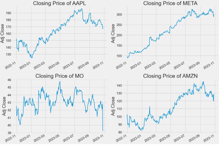
- Closing price charts of portfolio 1
# Let's see a historical view of the closing price
plt.figure(figsize=(15, 10))
plt.rcParams.update({'font.size': 18})
plt.subplots_adjust(top=1.25, bottom=1.2)

plt.rc('xtick', labelsize=16) #fontsize of the x tick labels
plt.rc('ytick', labelsize=16) #fontsize of the y tick labels

for i, company in enumerate(company_list, 1):
    plt.subplot(2, 2, i)
    company['Adj Close'].plot(linewidth=2)
    plt.ylabel('Adj Close')
    plt.xlabel(None)
    plt.title(f"Closing Price of {tech_list[i - 1]}")


plt.tight_layout()
- Sales volumes of portfolio 1
# Now let's plot the total volume of stock being traded each day
plt.figure(figsize=(15, 10))
plt.subplots_adjust(top=1.25, bottom=1.2)

for i, company in enumerate(company_list, 1):
    plt.subplot(2, 2, i)
    company['Volume'].plot(linewidth=2)
    plt.ylabel('Volume')
    plt.xlabel(None)
    plt.title(f"Sales Volume for {tech_list[i - 1]}")

plt.tight_layout()

- MAs of portfolio 1 for 10-20-50 days
ma_day = [10, 20, 50]

for ma in ma_day:
    for company in company_list:
        column_name = f"MA for {ma} days"
        company[column_name] = company['Adj Close'].rolling(ma).mean()


fig, axes = plt.subplots(nrows=2, ncols=2)
fig.set_figheight(10)
fig.set_figwidth(15)

AAPL[['Adj Close', 'MA for 10 days', 'MA for 20 days', 'MA for 50 days']].plot(ax=axes[0,0],linewidth=2)
axes[0,0].set_title('APPLE')

META[['Adj Close', 'MA for 10 days', 'MA for 20 days', 'MA for 50 days']].plot(ax=axes[0,1],linewidth=2)
axes[0,1].set_title('META')

MO[['Adj Close', 'MA for 10 days', 'MA for 20 days', 'MA for 50 days']].plot(ax=axes[1,0],linewidth=2)
axes[1,0].set_title('ALTRIA')

AMZN[['Adj Close', 'MA for 10 days', 'MA for 20 days', 'MA for 50 days']].plot(ax=axes[1,1],linewidth=2)
axes[1,1].set_title('AMAZON')

fig.tight_layout()

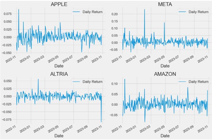
- Daily returns of portfolio 1 as line charts
#What was the daily return of the stock on average?
# We'll use pct_change to find the percent change for each day
for company in company_list:
    company['Daily Return'] = company['Adj Close'].pct_change()

# Then we'll plot the daily return percentage
fig, axes = plt.subplots(nrows=2, ncols=2)
fig.set_figheight(10)
fig.set_figwidth(15)

AAPL['Daily Return'].plot(ax=axes[0,0], legend=True, linestyle='-', linewidth=2)
axes[0,0].set_title('APPLE')

META['Daily Return'].plot(ax=axes[0,1], legend=True, linestyle='-', linewidth=2)
axes[0,1].set_title('META')

MO['Daily Return'].plot(ax=axes[1,0], legend=True, linestyle='-', linewidth=2)
axes[1,0].set_title('ALTRIA')

AMZN['Daily Return'].plot(ax=axes[1,1], legend=True, linestyle='-', linewidth=2)
axes[1,1].set_title('AMAZON')

fig.tight_layout()
- Daily returns of portfolio 1 as histograms
plt.figure(figsize=(12, 9))

for i, company in enumerate(company_list, 1):
    plt.subplot(2, 2, i)
    company['Daily Return'].hist(bins=50)
    plt.xlabel('Daily Return')
    plt.ylabel('Counts')
    plt.title(f'{company_name[i - 1]}')

plt.tight_layout()

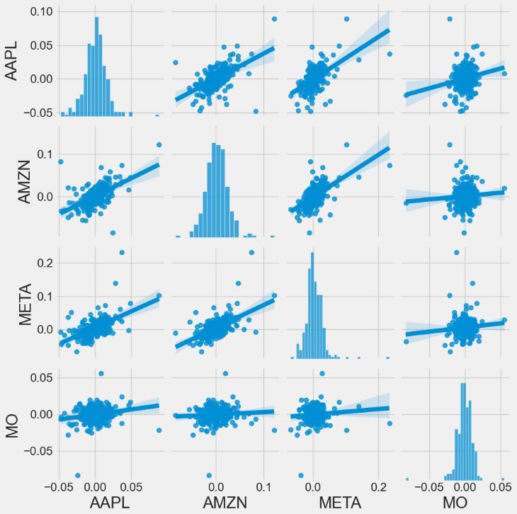
- Stock correlations of portfolio 1
#What was the correlation between different stocks closing prices?
# Grab all the closing prices for the tech stock list into one DataFrame

closing_df = pdr.get_data_yahoo(tech_list, start=start, end=end)['Adj Close']

# Make a new tech returns DataFrame
tech_rets = closing_df.pct_change()
tech_rets.head()
[*********************100%***********************]  4 of 4 completed

# We can simply call pairplot on our DataFrame for an automatic visual analysis
# of all the comparisons

sns.pairplot(tech_rets, kind='reg')
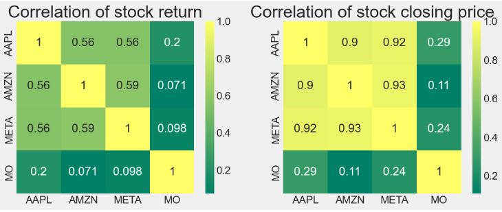
- Correlation matrix of portfolio 1: stock returns vs closing price
plt.figure(figsize=(12, 10))

plt.subplot(2, 2, 1)
sns.heatmap(tech_rets.corr(), annot=True, cmap='summer')
plt.title('Correlation of stock return')

plt.subplot(2, 2, 2)
sns.heatmap(closing_df.corr(), annot=True, cmap='summer')
plt.title('Correlation of stock closing price')
- Risk-return mapping of portfolio 1
#How much value do we put at risk by investing in a particular stock?
rets = tech_rets.dropna()

area = np.pi * 20

plt.figure(figsize=(10, 8))
plt.scatter(rets.mean(), rets.std(), s=area)
plt.xlabel('Expected return')
plt.ylabel('Risk')

for label, x, y in zip(rets.columns, rets.mean(), rets.std()):
    plt.annotate(label, xy=(x, y), xytext=(50, 50), textcoords='offset points', ha='right', va='bottom',
                 arrowprops=dict(arrowstyle='-', color='blue', connectionstyle='arc3,rad=-0.3'))
plt.grid(lw=3)

plt.show()

Portfolio 2: (DIS, AMD) + (AAPL, TSLA)
- In this section, we will invoke Quantstats to optimize portfolio 2 that consists of Apple, Tesla, The Walt Disney Company, and AMD stocks.
- Reading input stock data from yfinance
import yfinance as yf
startdate='2020-01-01'
enddate='2023-10-27'
# Getting dataframes info for Stocks using yfinance
aapl_df = yf.download('AAPL', start = startdate, end = enddate)
tsla_df = yf.download('TSLA', start = startdate, end = enddate)
dis_df = yf.download('NVDA', start = startdate, end = enddate)
amd_df = yf.download('META', start = startdate, end = enddate)

[*********************100%***********************]  1 of 1 completed
[*********************100%***********************]  1 of 1 completed
[*********************100%***********************]  1 of 1 completed
[*********************100%***********************]  1 of 1 completed
# Extracting Adjusted Close for each stock
aapl_df = aapl_df['Adj Close']
tsla_df = tsla_df['Adj Close']
dis_df = dis_df['Adj Close']
amd_df = amd_df['Adj Close']
# Merging and creating an Adj Close dataframe for stocks
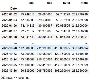
df = pd.concat([aapl_df, tsla_df, dis_df, amd_df], join = 'outer', axis = 1)
df.columns = ['aapl', 'tsla', 'nvda', 'meta']
df # Visualizing dataframe for input
- Optimizing portfolio 2 in terms of max Sharpe ratio and Efficient Frontier
# Importing libraries for portfolio optimization
from pypfopt.efficient_frontier import EfficientFrontier
from pypfopt import risk_models
from pypfopt import expected_returns
# Calculating the annualized expected returns and the annualized sample covariance matrix
mu = expected_returns.mean_historical_return(df) #expected returns
S = risk_models.sample_cov(df) #Covariance matrix
# Visualizing the annualized expected returns
mu

aapl    0.241023
tsla    0.676460
nvda    0.649880
meta    0.086997
dtype: float64
# Visualizing the covariance matrix
S

          aapl	      tsla	    nvda	     meta
aapl	0.116819	0.121311	0.126178	0.098940
tsla	0.121311	0.477221	0.200507	0.120923
nvda	0.126178	0.200507	0.303958	0.148242
meta	0.098940	0.120923	0.148242	0.226365
# Optimizing for maximal Sharpe ratio
ef = EfficientFrontier(mu, S) # Providing expected returns and covariance matrix as input
weights = ef.max_sharpe() # Optimizing weights for Sharpe ratio maximization

clean_weights = ef.clean_weights() # clean_weights rounds the weights and clips near-zeros

# Printing optimized weights and expected performance for portfolio
clean_weights

OrderedDict([('aapl', 0.0),
             ('tsla', 0.30239),
             ('nvda', 0.69761),
             ('meta', 0.0)])
#Original portfolio (benchmark)
portfolio = tsla_df*0.25 + dis_df*0.25+aapl_df*0.25+amd_df*0.25
# Creating new portfolio with optimized weights
new_weights = [0.65871, 0.34129]
optimized_portfolio = tsla_df*new_weights[0] + aapl_df*new_weights[1]
optimized_portfolio # Visualizing daily returns

Date
2020-01-02     43.893594
2020-01-03     44.210453
2020-01-06     44.782306
2020-01-07     45.434324
2020-01-08     46.847374
                 ...
2023-10-20    198.642153
2023-10-23    198.742388
2023-10-24    201.817230
2023-10-25    198.317898
2023-10-26    192.494054
Name: Adj Close, Length: 962, dtype: float64
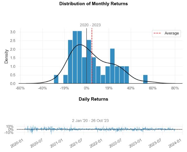
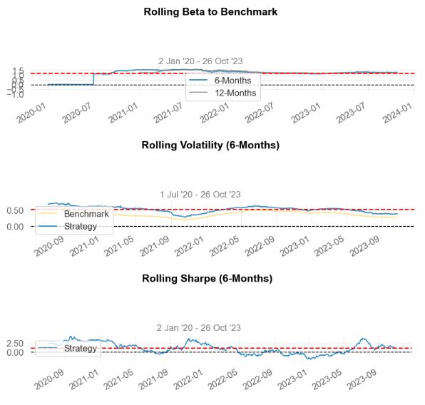
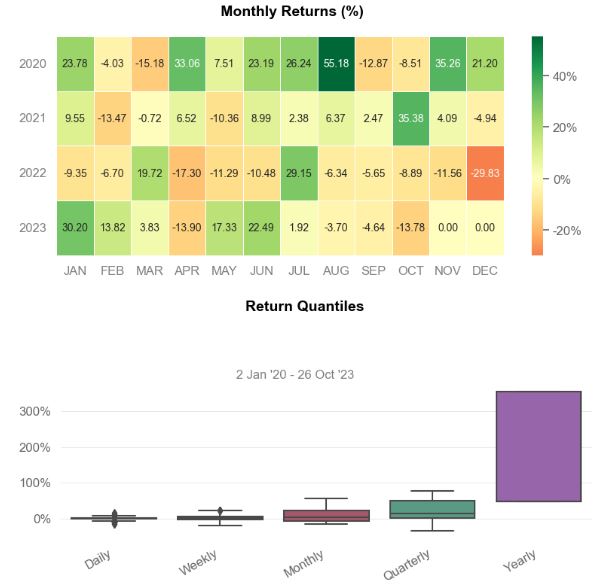
# Displaying new reports comparing the optimized portfolio to the first portfolio constructed
from IPython.core.display import display, HTML
display(HTML("<style>div.output_scroll { height: 144em; }</style>"))
import quantstats as qs
qs.reports.full(optimized_portfolio, benchmark = portfolio)
Performance Metrics
                           Strategy    Benchmark
-------------------------  ----------  -----------
Start Period               2020-01-02  2020-01-02
End Period                 2023-10-26  2023-10-26
Risk-Free Rate             0.0%        0.0%
Time in Market             100.0%      100.0%

Cumulative Return          338.55%     82.5%
CAGR﹪                     47.31%      17.07%

Sharpe                     0.99        0.6
Prob. Sharpe Ratio         97.28%      87.8%
Smart Sharpe               0.94        0.57
Sortino                    1.45        0.85
Smart Sortino              1.38        0.81
Sortino/√2                 1.02        0.6
Smart Sortino/√2           0.98        0.57
Omega                      1.19        1.19

Max Drawdown               -65.0%      -56.61%
Longest DD Days            660         660
Volatility (ann.)          53.88%      39.1%
R^2                        0.86        0.86
Information Ratio          0.08        0.08
Calmar                     0.73        0.3
Skew                       -0.13       -0.24
Kurtosis                   2.21        2.38

Expected Daily %           0.15%       0.06%
Expected Monthly %         3.27%       1.32%
Expected Yearly %          44.71%      16.23%
Kelly Criterion            7.65%       4.69%
Risk of Ruin               0.0%        0.0%
Daily Value-at-Risk        -5.37%      -3.96%
Expected Shortfall (cVaR)  -5.37%      -3.96%

Max Consecutive Wins       13          11
Max Consecutive Losses     8           8
Gain/Pain Ratio            0.19        0.11
Gain/Pain (1M)             0.97        0.53

Payoff Ratio               1.01        0.93
Profit Factor              1.19        1.11
Common Sense Ratio         1.25        1.08
CPC Index                  0.64        0.56
Tail Ratio                 1.05        0.97
Outlier Win Ratio          3.0         4.24
Outlier Loss Ratio         3.15        4.11

MTD                        -13.78%     -9.78%
3M                         -20.04%     -16.91%
6M                         19.14%      7.97%
YTD                        53.63%      35.1%
1Y                         -2.88%      1.19%
3Y (ann.)                  5.44%       0.3%
5Y (ann.)                  47.31%      17.07%
10Y (ann.)                 47.31%      17.07%
All-time (ann.)            47.31%      17.07%

Best Day                   15.9%       12.86%
Worst Day                  -16.67%     -12.25%
Best Month                 55.18%      30.87%
Worst Month                -29.83%     -21.91%
Best Year                  354.51%     113.44%
Worst Year                 -57.1%      -51.11%

Avg. Drawdown              -10.07%     -7.7%
Avg. Drawdown Days         50          51
Recovery Factor            5.21        1.46
Ulcer Index                0.28        0.25
Serenity Index             0.85        0.18

Avg. Up Month              19.01%      11.77%
Avg. Down Month            -10.16%     -7.98%
Win Days %                 53.69%      54.01%
Win Month %                52.17%      50.0%
Win Quarter %              68.75%      56.25%
Win Year %                 75.0%       75.0%

Beta                       1.27        -
Alpha                      0.23        -
Correlation                92.49%      -
Treynor Ratio              265.64%     -
None
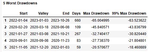
5 Worst Drawdowns
       Start	Valley	     End	   Days	Max Drawdown  99% Max Drawdown
1	2022-01-04	2023-01-03	2023-10-26	660	-65.004995	-63.523622
2	2020-02-20	2020-03-18	2020-06-08	109	-45.840571	-43.836799
3	2021-01-27	2021-03-08	2021-10-21	267	-32.740417	-30.820440
4	2020-09-01	2020-09-08	2020-11-23	83	-27.738370	-21.804801
5	2021-11-05	2021-12-20	2022-01-03	59	-20.570677	-18.460889


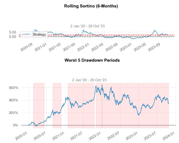

- Let’s build the entire portfolio optimization (PO) pipeline
# Importing libraries
import pandas as pd
import numpy as np
import quantstats as qs
import matplotlib.pyplot as plt
import seaborn as sns
from sklearn.linear_model import LinearRegression
import plotly.express as px
import yfinance as yf
# Getting daily returns for 4 different US stocks in the same time window
aapl = qs.utils.download_returns('AAPL')
aapl = aapl.loc[startdate:enddate]

tsla = qs.utils.download_returns('TSLA')
tsla = tsla.loc[startdate:enddate]

dis = qs.utils.download_returns('DIS')
dis = dis.loc[startdate:enddate]

amd = qs.utils.download_returns('AMD')
amd = amd.loc[startdate:enddate]
# Plotting Daily Returns for each stock
print('\nApple Daily Returns Plot:\n')
qs.plots.daily_returns(aapl)
print('\nTesla Inc. Daily Returns Plot:\n')
qs.plots.daily_returns(tsla)
print('\nThe Walt Disney Company Daily Returns Plot:\n')
qs.plots.daily_returns(dis)
print('\nAdvances Micro Devices, Inc. Daily Returns Plot:\n')
qs.plots.daily_returns(amd)


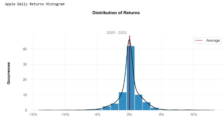
- Plotting histograms of the above daily returns
# Plotting histograms
from IPython.core.display import display, HTML
display(HTML("<style>div.output_scroll { height: 144em; }</style>"))
print('\nApple Daily Returns Histogram')
qs.plots.histogram(aapl, resample = 'D')
print('\nTesla Inc. Daily Returns Histogram')
qs.plots.histogram(tsla, resample = 'D')
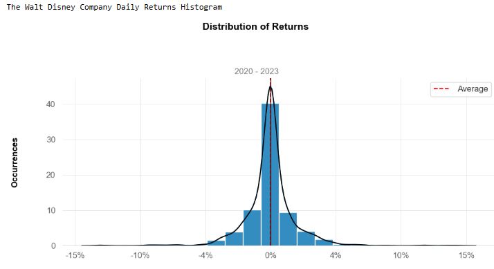
print('\nThe Walt Disney Company Daily Returns Histogram')
qs.plots.histogram(dis, resample = 'D')
print('\nAdvances Micro Devices, Inc. Daily Returns Histogram')
qs.plots.histogram(amd, resample = 'D')


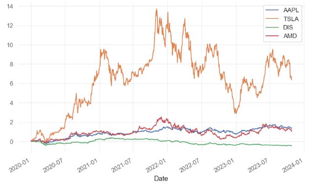
- Comparing cumulative returns of these 4 stocks in a single line plot
fig, ax = plt.subplots()
((aapl + 1).cumprod() - 1).plot(ax=ax)
((tsla + 1).cumprod() - 1).plot(ax=ax)
((dis + 1).cumprod() - 1).plot(ax=ax)
((amd + 1).cumprod() - 1).plot(ax=ax)
ax.legend(["AAPL","TSLA","DIS","AMD"]);
- Comparing STD, kurtosis, and skewness of these 4 stocks
# Using quantstats to measure kurtosis
print("Apple's kurtosis: ", qs.stats.kurtosis(aapl).round(2))
print("Tesla's kurtosis: ", qs.stats.kurtosis(tsla).round(2))
print("Walt Disney's kurtosis: ", qs.stats.kurtosis(dis).round(3))
print("Advances Micro Devices' kurtosis: ", qs.stats.kurtosis(amd).round(3))

Apple's kurtosis:  4.67
Tesla's kurtosis:  2.78
Walt Disney's kurtosis:  7.357
Advances Micro Devices' kurtosis:  2.1
# Measuring skewness with quantstats
print("Apple's skewness: ", qs.stats.skew(aapl).round(2))
print("Tesla's skewness: ", qs.stats.skew(tsla).round(2))
print("Walt Disney's skewness: ", qs.stats.skew(dis).round(3))
print("Advances Micro Devices' skewness: ", qs.stats.skew(amd).round(3))

Apple's skewness:  0.08
Tesla's skewness:  0.08
Walt Disney's skewness:  0.28
Advances Micro Devices' skewness:  0.202
# Calculating Standard Deviations
print("Apple's Standard Deviation: ", aapl.std())
print("\nTesla's Standard Deviation: ", tsla.std())
print("\nDisney's Standard Deviation: ", dis.std())
print("\nAMD's Standard Deviation: ", amd.std())

Apple's Standard Deviation:  0.021520708530783472
Tesla's Standard Deviation:  0.043479817357367966
Disney's Standard Deviation:  0.02271810742856512
AMD's Standard Deviation:  0.03403554120470168
- Let’s compare portfolio 2 against the most popular S&P 500 benchmark
# Loading data from the SP500, the American benchmark
sp500 = qs.utils.download_returns('^GSPC')
sp500 = sp500.loc[startdate:enddate]
sp500.index = sp500.index.tz_convert(None)
aapl_no_index=aapl.reset_index(drop=True)
sp500_no_index=sp500.reset_index(drop=True)
# Fitting linear relation among Apple's returns and Benchmark
X = sp500_no_index.values.reshape(-1,1)
y = aapl_no_index.values.reshape(-1,1)

linreg = LinearRegression().fit(X, y)

beta = linreg.coef_[0]
alpha = linreg.intercept_

print('AAPL beta: ', beta.round(3))
print('\nAAPL alpha: ', alpha.round(3))
AAPL beta:  [1.194]

AAPL alpha:  [0.001]
tsla_no_index=tsla.reset_index(drop=True)
dis_no_index=dis.reset_index(drop=True)
amd_no_index=amd.reset_index(drop=True)
X = sp500_no_index.values.reshape(-1,1)
y = tsla_no_index.values.reshape(-1,1)

linreg = LinearRegression().fit(X, y)

beta = linreg.coef_[0]
alpha = linreg.intercept_

print('TSLA beta: ', beta.round(3))
print('\nTSLA alpha: ', alpha.round(3))
TSLA beta:  [1.516]

TSLA alpha:  [0.002]
X = sp500_no_index.values.reshape(-1,1)
y = dis_no_index.values.reshape(-1,1)

linreg = LinearRegression().fit(X, y)

beta = linreg.coef_[0]
alpha = linreg.intercept_

print('DIS beta: ', beta.round(3))
print('\nDIS alpha: ', alpha.round(3))
DIS beta:  [1.075]

DIS alpha:  [-0.001]
X = sp500_no_index.values.reshape(-1,1)
y = amd_no_index.values.reshape(-1,1)

linreg = LinearRegression().fit(X, y)

beta = linreg.coef_[0]
alpha = linreg.intercept_

print('AMD beta: ', beta.round(3))
print('\nAMD alpha: ', alpha.round(3))
AMD beta:  [1.508]

AMD alpha:  [0.001]
- Calculating the Sharpe Ratio
# Calculating the Sharpe ratio
print("Sharpe Ratio for AAPL: ", qs.stats.sharpe(aapl).round(2))
print("Sharpe Ratio for TSLA: ", qs.stats.sharpe(tsla).round(2))
print("Sharpe Ratio for DIS: ", qs.stats.sharpe(dis).round(2))
print("Sharpe Ratio for AMD: ", qs.stats.sharpe(amd).round(2))
Sharpe Ratio for AAPL:  0.82
Sharpe Ratio for TSLA:  1.11
Sharpe Ratio for DIS:  -0.26
Sharpe Ratio for AMD:  0.63

- Summary of the Portfolio Optimization (PO) workflow applied to portfolio 2
# Getting dataframes info for Stocks using yfinance
aapl_df = yf.download('AAPL', start = startdate, end = enddate)
tsla_df = yf.download('TSLA', start = startdate, end = enddate)
dis_df = yf.download('DIS', start = startdate, end = enddate)
amd_df = yf.download('AMD', start = startdate, end = enddate)

# Extracting Adjusted Close for each stock
aapl_df = aapl_df['Adj Close']
tsla_df = tsla_df['Adj Close']
dis_df = dis_df['Adj Close']
amd_df = amd_df['Adj Close']

# Merging and creating an Adj Close dataframe for stocks
df = pd.concat([aapl_df, tsla_df, dis_df, amd_df], join = 'outer', axis = 1)
df.columns = ['aapl', 'tsla', 'dis', 'amd']

# Importing libraries for portfolio optimization
from pypfopt.efficient_frontier import EfficientFrontier
from pypfopt import risk_models
from pypfopt import expected_returns

# Calculating the annualized expected returns and the annualized sample covariance matrix
mu = expected_returns.mean_historical_return(df) #expected returns
S = risk_models.sample_cov(df) #Covariance matrix

# Visualizing the annualized expected returns
mu
aapl    0.241023
tsla    0.676460
dis    -0.149894
amd     0.184567
dtype: float64

# Visualizing the covariance matrix
S
           aapl	    tsla	         dis	amd
aapl	0.116818	0.121311	0.060739	0.112920
tsla	0.121311	0.477221	0.088326	0.180042
dis	0.060739	0.088326	0.130159	0.077896
amd	0.112920	0.180042	0.077896	0.291059

# Optimizing for maximal Sharpe ratio
ef = EfficientFrontier(mu, S) # Providing expected returns and covariance matrix as input
weights = ef.max_sharpe() # Optimizing weights for Sharpe ratio maximization

clean_weights = ef.clean_weights() # clean_weights rounds the weights and clips near-zeros

# Printing optimized weights and expected performance for portfolio
clean_weights

rderedDict([('aapl', 0.34129), ('tsla', 0.65871), ('dis', 0.0), ('amd', 0.0)])

#Benchmark portfolio
portfolio = aapl*0.25 + tsla*0.25+dis*0.25+amd*0.25
# Creating new portfolio with optimized weights
new_weights = [0.34129, 0.65871]
optimized_portfolio = aapl*new_weights[0] + tsla*new_weights[1]
optimized_portfolio # Visualizing daily returns
- Comparing portfolio 2 cumulative returns % before and after portfolio optimization (PO)
# Displaying new reports comparing the optimized portfolio to the first portfolio constructed
#https://stackoverflow.com/questions/40204396/plot-cumulative-returns-of-a-pandas-dataframe
fig, ax = plt.subplots()
((optimized_portfolio  + 1).cumprod() - 1).plot(ax=ax)
((portfolio  + 1).cumprod() - 1).plot(ax=ax)
ax.legend(["After PO","Before PO"]);
plt.title('Portfolio Cumulative Return')

AAPL Price LSTM Forecasting
- It appears that AAPL is the most appealing asset of portfolio 1 in terms of risk/return balance.
- Let’s predict the AAPL price using Keras LSTM
#Predicting the closing price stock price of APPLE inc:
# Get the stock quote
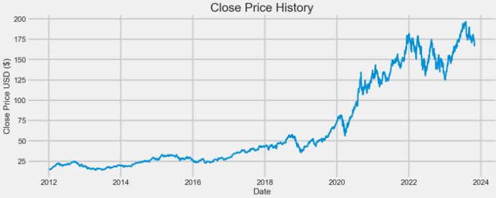
df = pdr.get_data_yahoo('AAPL', start='2012-01-01', end=datetime.now())
[*********************100%***********************] 1 of 1 completed
plt.figure(figsize=(16,6))
plt.title('Close Price History')
plt.plot(df['Close'],linewidth=3)
plt.xlabel('Date', fontsize=18)
plt.ylabel('Close Price USD ($)', fontsize=18)
plt.grid(lw=3)
plt.show()
- Train/test data preparation
# Create a new dataframe with only the 'Close column
data = df.filter(['Close'])
# Convert the dataframe to a numpy array
dataset = data.values
# Get the number of rows to train the model on
training_data_len = int(np.ceil( len(dataset) * .95 ))

training_data_len
2828
# Scale the data
from sklearn.preprocessing import StandardScaler

#scaler = MinMaxScaler(feature_range=(0,1))
scaler = StandardScaler()
scaled_data = scaler.fit_transform(dataset)
# Create the training data set
# Create the scaled training data set
train_data = scaled_data[0:int(training_data_len), :]
# Split the data into x_train and y_train data sets
x_train = []
y_train = []

for i in range(60, len(train_data)):
    x_train.append(train_data[i-60:i, 0])
    y_train.append(train_data[i, 0])
    if i<= 61:
        print(x_train)
        print(y_train)
        print()

# Convert the x_train and y_train to numpy arrays
x_train, y_train = np.array(x_train), np.array(y_train)

# Reshape the data
x_train = np.reshape(x_train, (x_train.shape[0], x_train.shape[1], 1))
# Create the testing data set
# Create a new array containing scaled values from index 1543 to 2002
test_data = scaled_data[training_data_len - 60: , :]
# Create the data sets x_test and y_test
x_test = []
y_test = dataset[training_data_len:, :]
for i in range(60, len(test_data)):
    x_test.append(test_data[i-60:i, 0])

# Convert the data to a numpy array
x_test = np.array(x_test)

# Reshape the data
x_test = np.reshape(x_test, (x_test.shape[0], x_test.shape[1], 1 ))
- Train the model and get test predictions
from keras.models import Sequential
from keras.layers import Dense, LSTM

# Build the LSTM model
model = Sequential()
model.add(LSTM(128, return_sequences=True, input_shape= (x_train.shape[1], 1)))
model.add(LSTM(64, return_sequences=False))
model.add(Dense(25))
model.add(Dense(1))

# Compile the model
model.compile(optimizer='adam', loss='mean_squared_error')

# Train the model
model.fit(x_train, y_train, batch_size=1, epochs=1)

2768/2768 [==============================] - 38s 13ms/step - loss: 0.0081
# Get the models predicted price values
predictions = model.predict(x_test)
predictions = scaler.inverse_transform(predictions)

# Get the root mean squared error (RMSE)
rmse = np.sqrt(np.mean(((predictions - y_test) ** 2)))
rmse

5.9636350262044076
# Plot the data
train = data[:training_data_len]
valid = data[training_data_len:]
valid['Predictions'] = predictions
# Visualize the data
plt.figure(figsize=(16,6))
plt.title('Model')
plt.xlabel('Date', fontsize=18)
plt.ylabel('Close Price USD ($)', fontsize=18)
plt.plot(train['Close'],linewidth=3)
plt.plot(valid[['Close', 'Predictions']],linewidth=3)
plt.legend(['Train', 'Val', 'Predictions'], loc='lower right')
plt.grid(lw=3)
plt.show()

NVDA Entry/Exit Trading Signals
- In this section, we will implement the NVIDIA trading dashboard with Yfinance & Python
# Import libraries and dependencies
import numpy as np
import pandas as pd
import hvplot.pandas
from pathlib import Path
import yfinance as yf
#Define ticker
net = yf.Ticker("NVDA")
net
# Set the timeframe you are interested in viewing.
net_historical = net.history(start="2020-01-1", end="2023-10-30", interval="1d")
# Create a new DataFrame called signals, keeping only the 'Date' & 'Close' columns.
signals_df = net_historical.drop(columns=['Open', 'High', 'Low', 'Volume','Dividends', 'Stock Splits'])
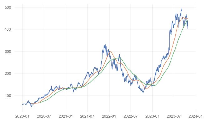
- Calculating the short/long window smooth moving averages (SMAs) for 50 and 100 days
# Set the short window and long windows
short_window = 50
long_window = 100
# Generate the short and long moving averages (50 and 100 days, respectively)
signals_df['SMA50'] = signals_df['Close'].rolling(window=short_window).mean()
signals_df['SMA100'] = signals_df['Close'].rolling(window=long_window).mean()
signals_df['Signal'] = 0.0
# Generate the trading signal 0 or 1,
# where 0 is when the SMA50 is under the SMA100, and
# where 1 is when the SMA50 is higher (or crosses over) the SMA100
signals_df['Signal'][short_window:] = np.where(
    signals_df['SMA50'][short_window:] > signals_df['SMA100'][short_window:], 1.0, 0.0
)
# Calculate the points in time at which a position should be taken, 1 or -1
signals_df['Entry/Exit'] = signals_df['Signal'].diff()
# Print the DataFrame
signals_df.tail(10)

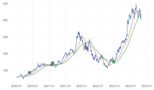
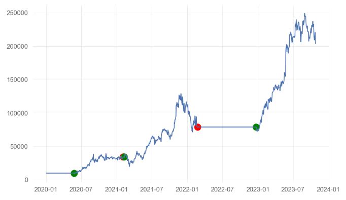
- Plotting the Entry/Exit trading signals
signals_df1=signals_df.reset_index()
# Visualize exit position relative to close price
sigx=signals_df1[signals_df1['Entry/Exit'] == -1.0]['Date']
sigy=signals_df1[signals_df1['Entry/Exit'] == -1.0]['Close']
plt.scatter(sigx,sigy,s=170,c='r')

sigx=signals_df1[signals_df1['Entry/Exit'] == 1.0]['Date']
sigy=signals_df1[signals_df1['Entry/Exit'] == 1.0]['Close']
plt.scatter(sigx,sigy,s=170,c='g')

sigx=signals_df1['Date']
sigy=signals_df1['Close']
plt.plot(sigx,sigy)

sigx=signals_df1['Date']
sigy=signals_df1['SMA50']
plt.plot(sigx,sigy)

sigx=signals_df1['Date']
sigy=signals_df1['SMA100']
plt.plot(sigx,sigy)
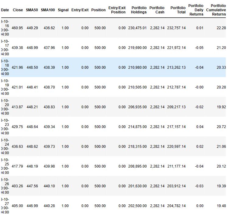
- Calculating the portfolio returns by setting initial_capital = float(10000)
# Set initial capital
initial_capital = float(10000)
# Set the share size
share_size = 500
# Take a 500 share position where the dual moving average crossover is 1 (SMA50 is greater than SMA100)
signals_df1['Position'] = share_size * signals_df1['Signal']
# Find the points in time where a 500 share position is bought or sold
signals_df1['Entry/Exit Position'] = signals_df1['Position'].diff()
# Multiply share price by entry/exit positions and get the cumulatively sum
signals_df1['Portfolio Holdings'] = signals_df1['Close'] * signals_df1['Entry/Exit Position'].cumsum()
# Subtract the initial capital by the portfolio holdings to get the amount of liquid cash in the portfolio
signals_df1['Portfolio Cash'] = initial_capital - (signals_df1['Close'] * signals_df1['Entry/Exit Position']).cumsum()
# Get the total portfolio value by adding the cash amount by the portfolio holdings (or investments)
signals_df1['Portfolio Total'] = signals_df1['Portfolio Cash'] + signals_df1['Portfolio Holdings']
# Calculate the portfolio daily returns
signals_df1['Portfolio Daily Returns'] = signals_df1['Portfolio Total'].pct_change()
# Calculate the cumulative returns
signals_df1['Portfolio Cumulative Returns'] = (1 + signals_df1['Portfolio Daily Returns']).cumprod() - 1
# Print the DataFrame
signals_df1.tail(10)
- Plotting portfolio cumulative returns vs trading signals
sigx=signals_df1[signals_df1['Entry/Exit'] == -1.0]['Date']
sigy=signals_df1[signals_df1['Entry/Exit'] == -1.0]['Portfolio Total']
plt.scatter(sigx,sigy,s=150,c='red')
sigx=signals_df1[signals_df1['Entry/Exit'] == 1.0]['Date']
sigy=signals_df1[signals_df1['Entry/Exit'] == 1.0]['Portfolio Total']
plt.scatter(sigx,sigy,s=150,c='green')
sigx=signals_df1['Date']
sigy=signals_df1['Portfolio Total']
plt.plot(sigx,sigy)
- Initiating the NVDA portfolio evaluation process based on signals_df1
# Prepare DataFrame for metrics
metrics = [
    'Annual Return',
    'Cumulative Returns',
    'Annual Volatility',
    'Sharpe Ratio',
    'Sortino Ratio']
columns = ['Backtest']
# Initialize the DataFrame with index set to evaluation metrics and column as `Backtest` (just like PyFolio)
portfolio_evaluation_df = pd.DataFrame(index=metrics, columns=columns)
# Calculate cumulative return
portfolio_evaluation_df.loc['Cumulative Returns'] = signals_df1['Portfolio Cumulative Returns'].iloc[-1]
# Calculate annualized return
portfolio_evaluation_df.loc['Annual Return'] = (
    signals_df1['Portfolio Daily Returns'].mean() * 252
)
# Calculate annual volatility
portfolio_evaluation_df.loc['Annual Volatility'] = (
    signals_df1['Portfolio Daily Returns'].std() * np.sqrt(252)
)
# Calculate Sharpe Ratio
portfolio_evaluation_df.loc['Sharpe Ratio'] = (
    signals_df1['Portfolio Daily Returns'].mean() * 252) / (
    signals_df1['Portfolio Daily Returns'].std() * np.sqrt(252)
)
# Calculate Downside Return
sortino_ratio_df = signals_df1[['Portfolio Daily Returns']].copy()
sortino_ratio_df.loc[:,'Downside Returns'] = 0
target = 0
mask = sortino_ratio_df['Portfolio Daily Returns'] < target
sortino_ratio_df.loc[mask, 'Downside Returns'] = sortino_ratio_df['Portfolio Daily Returns']**2
portfolio_evaluation_df
# Calculate Sortino Ratio
down_stdev = np.sqrt(sortino_ratio_df['Downside Returns'].mean()) * np.sqrt(252)
expected_return = sortino_ratio_df['Portfolio Daily Returns'].mean() * 252
sortino_ratio = expected_return/down_stdev
portfolio_evaluation_df.loc['Sortino Ratio'] = sortino_ratio
portfolio_evaluation_df.head()


	              Backtest
--------------------------
Annual Return	    1.01
Cumulative Returns	19.48
Annual Volatility	0.66
Sharpe Ratio	    1.53
Sortino Ratio	    2.47
# Initialize trade evaluation DataFrame with columns.
trade_evaluation_df = pd.DataFrame(
    columns=[
        'Stock',
        'Entry Date',
        'Exit Date',
        'Shares',
        'Entry Share Price',
        'Exit Share Price',
        'Entry Portfolio Holding',
        'Exit Portfolio Holding',
        'Profit/Loss']
)

print (row)

Close        403.26
SMA50        447.56
SMA100       440.10
Signal         1.00
Entry/Exit     0.00
Name: 2023-10-26 00:00:00-04:00, dtype: float64
# Initialize iterative variables
entry_date = ''
exit_date = ''
entry_portfolio_holding = 0
exit_portfolio_holding = 0
share_size = 0
entry_share_price = 0
exit_share_price = 0

for index, row in signals_df.iterrows():
    if row['Entry/Exit'] == 1:
        entry_date = index
        entry_portfolio_holding = abs(row['Close'] * row['Entry/Exit'])
        share_size = row['Entry/Exit']
        entry_share_price = row['Close']
    elif row['Entry/Exit'] == -1:
        exit_date = index
        exit_portfolio_holding = abs(row['Close'] * row['Entry/Exit'])
        exit_share_price = row['Close']
        profit_loss =  entry_portfolio_holding - exit_portfolio_holding
        trade_evaluation_df = trade_evaluation_df.append(
            {
                'Stock': 'NVDA',
                'Entry Date': entry_date,
                'Exit Date': exit_date,
                'Shares': share_size,
                'Entry Share Price': entry_share_price,
                'Exit Share Price': exit_share_price,
                'Entry Portfolio Holding': entry_portfolio_holding,
                'Exit Portfolio Holding': exit_portfolio_holding,
                'Profit/Loss': profit_loss
            },
            ignore_index=True)
price_df = signals_df[['Close', 'SMA50', 'SMA100']]
print(price_df)
                          Close  SMA50  SMA100
Date
2020-01-02 00:00:00-05:00  59.75    NaN     NaN
2020-01-03 00:00:00-05:00  58.79    NaN     NaN
2020-01-06 00:00:00-05:00  59.04    NaN     NaN
2020-01-07 00:00:00-05:00  59.75    NaN     NaN
2020-01-08 00:00:00-05:00  59.87    NaN     NaN
...                          ...    ...     ...
2023-10-23 00:00:00-04:00 429.75 448.64  439.34
2023-10-24 00:00:00-04:00 436.63 448.62  439.73
2023-10-25 00:00:00-04:00 417.79 448.19  439.98
2023-10-26 00:00:00-04:00 403.26 447.56  440.10
2023-10-27 00:00:00-04:00 405.00 446.99  440.28

[963 rows x 3 columns]
plt.plot(signals_df['Close'])
plt.plot(signals_df['SMA50'])
plt.plot(signals_df['SMA100']
portfolio_evaluation_df.reset_index(inplace=True)
print(portfolio_evaluation_df)

            index       Backtest
-------------------------------
0       Annual Return     1.01
1  Cumulative Returns    19.48
2   Annual Volatility     0.66
3        Sharpe Ratio     1.53
4       Sortino Ratio     2.47
NVDA Fundamental Analysis
- Based upon the highly encouraging outcome of the aforementioned NVDA portfolio evaluation procedure, let’s dive deeper into the stock’s fundamentals using the Financial Modeling Prep API:
#Retrieve Company Fundamentals with Python
import pandas as pd
import requests

pd.options.display.float_format = '{:,.2f}'.format

#pass ticker of the company

company = 'NVDA'

api = 'YOUR FMP API KEY'
# Request Financial Data from API and load to variables

IS = requests.get(f'https://financialmodelingprep.com/api/v3/income-statement/{company}?apikey={api}').json()

BS = requests.get(f'https://financialmodelingprep.com/api/v3/balance-sheet-statement/{company}?apikey={api}').json()

CF = requests.get(f'https://financialmodelingprep.com/api/v3/cash-flow-statement/{company}?apikey={api}').json()

Ratios = requests.get(f'https://financialmodelingprep.com/api/v3/ratios/{company}?apikey={api}').json()

key_Metrics = requests.get(f'https://financialmodelingprep.com/api/v3/key-metrics/{company}?apikey={api}').json()

profile = requests.get(f'https://financialmodelingprep.com/api/v3/profile/{company}?apikey={api}').json()

millions = 1000000
#Create empty dictionary and add the financials to it

financials = {}

dates = [2023,2022,2021,2020,2019]

for item in range(5):

    financials[dates[item]] ={}

#Key Metrics

    financials[dates[item]]['Mkt Cap'] = key_Metrics[item]['marketCap'] /millions

    financials[dates[item]]['Debt to Equity'] = key_Metrics[item]['debtToEquity']

    financials[dates[item]]['Debt to Assets'] = key_Metrics[item]['debtToAssets']

    financials[dates[item]]['Revenue per Share'] = key_Metrics[item]['revenuePerShare']

    financials[dates[item]]['NI per Share'] = key_Metrics[item]['netIncomePerShare']

    financials[dates[item]]['Revenue'] = IS[item]['revenue'] / millions

    financials[dates[item]]['Gross Profit'] = IS[item]['grossProfit'] / millions

    financials[dates[item]]['R&D Expenses'] = IS[item]['researchAndDevelopmentExpenses']/ millions

    financials[dates[item]]['Op Expenses'] = IS[item]['operatingExpenses'] / millions

    financials[dates[item]]['Op Income'] = IS[item]['operatingIncome'] / millions

    financials[dates[item]]['Net Income'] = IS[item]['netIncome'] / millions

    financials[dates[item]]['Cash'] = BS[item]['cashAndCashEquivalents'] / millions

    financials[dates[item]]['Inventory'] = BS[item]['inventory'] / millions

    financials[dates[item]]['Cur Assets'] = BS[item]['totalCurrentAssets'] / millions

    financials[dates[item]]['LT Assets'] = BS[item]['totalNonCurrentAssets'] / millions

    financials[dates[item]]['Int Assets'] = BS[item]['intangibleAssets'] / millions

    financials[dates[item]]['Total Assets'] = BS[item]['totalAssets'] / millions

    financials[dates[item]]['Cur Liab'] = BS[item]['totalCurrentLiabilities'] / millions

    financials[dates[item]]['LT Debt'] = BS[item]['longTermDebt'] / millions

    financials[dates[item]]['LT Liab'] = BS[item]['totalNonCurrentLiabilities'] / millions

    financials[dates[item]]['Total Liab'] = BS[item]['totalLiabilities'] / millions

    financials[dates[item]]['SH Equity'] = BS[item]['totalStockholdersEquity'] / millions

    financials[dates[item]]['CF Operations'] = CF[item]['netCashProvidedByOperatingActivities'] / millions

    financials[dates[item]]['CF Investing'] = CF[item]['netCashUsedForInvestingActivites'] / millions

    financials[dates[item]]['CF Financing'] = CF[item]['netCashUsedProvidedByFinancingActivities'] / millions

    financials[dates[item]]['CAPEX'] = CF[item]['capitalExpenditure'] / millions

    financials[dates[item]]['FCF'] = CF[item]['freeCashFlow'] / millions

    financials[dates[item]]['Dividends Paid'] = CF[item]['dividendsPaid'] / millions

#Income Statement Ratios

    financials[dates[item]]['Gross Profit Margin'] = Ratios[item]['grossProfitMargin']

    financials[dates[item]]['Op Margin'] = Ratios[item]['operatingProfitMargin']

    financials[dates[item]]['Int Coverage'] = Ratios[item]['interestCoverage']

    financials[dates[item]]['Net Profit Margin'] = Ratios[item]['netProfitMargin']

    financials[dates[item]]['Dividend Yield'] = Ratios[item]['dividendYield']

#BS Ratios

    financials[dates[item]]['Current Ratio'] = Ratios[item]['currentRatio']

    financials[dates[item]]['Operating Cycle'] = Ratios[item]['operatingCycle']

    financials[dates[item]]['Days of AP Outstanding'] = Ratios[item]['daysOfPayablesOutstanding']

    financials[dates[item]]['Cash Conversion Cycle'] = Ratios[item]['cashConversionCycle']

#Return Ratios

    financials[dates[item]]['ROA'] = Ratios[item]['returnOnAssets']

    financials[dates[item]]['ROE'] = Ratios[item]['returnOnEquity']

    financials[dates[item]]['ROCE'] = Ratios[item]['returnOnCapitalEmployed']

    financials[dates[item]]['Dividend Yield'] = Ratios[item]['dividendYield']

#Price Ratios

    financials[dates[item]]['PE'] = Ratios[item]['priceEarningsRatio']

    financials[dates[item]]['PS'] = Ratios[item]['priceToSalesRatio']

    financials[dates[item]]['PB'] = Ratios[item]['priceToBookRatio']

    financials[dates[item]]['Price To FCF'] = Ratios[item]['priceToFreeCashFlowsRatio']

    financials[dates[item]]['PEG'] = Ratios[item]['priceEarningsToGrowthRatio']

    financials[dates[item]]['EPS'] = IS[item]['eps']

    financials[dates[item]]['EPS'] = IS[item]['eps']

#Transform the dictionary into a Pandas

fundamentals = pd.DataFrame.from_dict(financials,orient='columns')
#Calculate Growth measures

fundamentals['CAGR'] = (fundamentals[2023]/fundamentals[2019])**(1/5) - 1

fundamentals['2023 growth'] = (fundamentals[2023] - fundamentals[2022] )/ fundamentals[2022]

fundamentals['2022 growth'] = (fundamentals[2022] - fundamentals[2021] )/ fundamentals[2021]

fundamentals['2021 growth'] = (fundamentals[2021] - fundamentals[2020] )/ fundamentals[2020]
fundamentals['2020 growth'] = (fundamentals[2020] - fundamentals[2019] )/ fundamentals[2019]

#Export to Excel

fundamentals.to_excel('fundamentalsnvda.xlsx')

print(fundamentals)
                             2023       2022       2021       2020      2019  \
Mkt Cap                476,558.94 611,170.56 326,689.16 146,281.80 83,904.00
Debt to Equity               0.54       0.44       0.45       0.22      0.22
Debt to Assets               0.29       0.26       0.26       0.15      0.16
Revenue per Share           10.85      10.78       6.76       4.48      4.82
NI per Share                 1.76       3.91       1.76       1.15      1.70
Revenue                 26,974.00  26,914.00  16,675.00  10,918.00 11,716.00
Gross Profit            15,356.00  17,475.00  10,396.00   6,768.00  7,171.00
R&D Expenses             7,339.00   5,268.00   3,924.00   2,829.00  2,376.00
Op Expenses              9,779.00   7,434.00   5,864.00   3,922.00  3,367.00
Op Income                4,224.00  10,041.00   4,532.00   2,846.00  3,804.00
Net Income               4,368.00   9,752.00   4,332.00   2,796.00  4,141.00
Cash                     3,389.00   1,990.00     847.00  10,896.00    782.00
Inventory                5,159.00   2,605.00   1,826.00     979.00  1,575.00
Cur Assets              23,073.00  28,829.00  16,055.00  13,690.00 10,557.00
LT Assets               18,109.00  15,358.00  12,736.00   3,625.00  2,735.00
Int Assets               1,676.00   2,339.00   2,737.00      49.00     45.00
Total Assets            41,182.00  44,187.00  28,791.00  17,315.00 13,292.00
Cur Liab                 6,563.00   4,335.00   3,925.00   1,784.00  1,329.00
LT Debt                 10,605.00  11,687.00   6,598.00   2,552.00  1,988.00
LT Liab                 12,518.00  13,240.00   7,973.00   3,327.00  2,621.00
Total Liab              19,081.00  17,575.00  11,898.00   5,111.00  3,950.00
SH Equity               22,101.00  26,612.00  16,893.00  12,204.00  9,342.00
CF Operations            5,641.00   9,108.00   5,822.00   4,761.00  3,743.00
CF Investing             7,375.00  -9,830.00 -19,675.00   6,145.00 -4,097.00
CF Financing           -11,617.00   1,865.00   3,804.00    -792.00 -2,866.00
CAPEX                   -1,833.00    -976.00  -1,128.00    -489.00   -600.00
FCF                      3,808.00   8,132.00   4,694.00   4,272.00  3,143.00
Dividends Paid            -398.00    -399.00    -395.00    -390.00   -371.00
Gross Profit Margin          0.57       0.65       0.62       0.62      0.61
Op Margin                    0.16       0.37       0.27       0.26      0.32
Int Coverage                16.12      42.55      24.63      54.73     65.59
Net Profit Margin            0.16       0.36       0.26       0.26      0.35
Dividend Yield               0.00       0.00       0.00       0.00      0.00
Current Ratio                3.52       6.65       4.09       7.67      7.94
Operating Cycle            213.86     163.80     159.31     141.50    170.85
Days of AP Outstanding      37.48      68.95      69.81      60.42     41.04
Cash Conversion Cycle      176.38      94.85      89.50      81.08    129.81
ROA                          0.11       0.22       0.15       0.16      0.31
ROE                          0.20       0.37       0.26       0.23      0.44
ROCE                         0.12       0.25       0.18       0.18      0.32
PE                         109.10      62.67      75.41      52.32     20.26
PS                          17.67      22.71      19.59      13.40      7.16
PB                          21.56      22.97      19.34      11.99      8.98
Price To FCF               125.15      75.16      69.60      34.24     26.70
PEG                         -1.98       0.51       1.42      -1.62      0.60
EPS                          1.76       3.91       1.76       1.15      1.70

                        CAGR  2023 growth  2022 growth  2021 growth  \
Mkt Cap                 0.42        -0.22         0.87         1.23
Debt to Equity          0.19         0.22        -0.02         1.08
Debt to Assets          0.13         0.09         0.00         0.73
Revenue per Share       0.18         0.01         0.60         0.51
NI per Share            0.01        -0.55         1.23         0.53
Revenue                 0.18         0.00         0.61         0.53
Gross Profit            0.16        -0.12         0.68         0.54
R&D Expenses            0.25         0.39         0.34         0.39
Op Expenses             0.24         0.32         0.27         0.50
Op Income               0.02        -0.58         1.22         0.59
Net Income              0.01        -0.55         1.25         0.55
Cash                    0.34         0.70         1.35        -0.92
Inventory               0.27         0.98         0.43         0.87
Cur Assets              0.17        -0.20         0.80         0.17
LT Assets               0.46         0.18         0.21         2.51
Int Assets              1.06        -0.28        -0.15        54.86
Total Assets            0.25        -0.07         0.53         0.66
Cur Liab                0.38         0.51         0.10         1.20
LT Debt                 0.40        -0.09         0.77         1.59
LT Liab                 0.37        -0.05         0.66         1.40
Total Liab              0.37         0.09         0.48         1.33
SH Equity               0.19        -0.17         0.58         0.38
CF Operations           0.09        -0.38         0.56         0.22
CF Investing             NaN        -1.75        -0.50        -4.20
CF Financing            0.32        -7.23        -0.51        -5.80
CAPEX                   0.25         0.88        -0.13         1.31
FCF                     0.04        -0.53         0.73         0.10
Dividends Paid          0.01        -0.00         0.01         0.01
Gross Profit Margin    -0.01        -0.12         0.04         0.01
Op Margin              -0.14        -0.58         0.37         0.04
Int Coverage           -0.24        -0.62         0.73        -0.55
Net Profit Margin      -0.14        -0.55         0.39         0.01
Dividend Yield         -0.28         0.28        -0.46        -0.55
Current Ratio          -0.15        -0.47         0.63        -0.47
Operating Cycle         0.05         0.31         0.03         0.13
Days of AP Outstanding -0.02        -0.46        -0.01         0.16
Cash Conversion Cycle   0.06         0.86         0.06         0.10
ROA                    -0.19        -0.52         0.47        -0.07
ROE                    -0.15        -0.46         0.43         0.12
ROCE                   -0.17        -0.52         0.38        -0.01
PE                      0.40         0.74        -0.17         0.44
PS                      0.20        -0.22         0.16         0.46
PB                      0.19        -0.06         0.19         0.61
Price To FCF            0.36         0.67         0.08         1.03
PEG                      NaN        -4.87        -0.64        -1.88
EPS                     0.01        -0.55         1.22         0.53

                        2020 growth
Mkt Cap                        0.74
Debt to Equity                -0.03
Debt to Assets                -0.02
Revenue per Share             -0.07
NI per Share                  -0.33
Revenue                       -0.07
Gross Profit                  -0.06
R&D Expenses                   0.19
Op Expenses                    0.16
Op Income                     -0.25
Net Income                    -0.32
Cash                          12.93
Inventory                     -0.38
Cur Assets                     0.30
LT Assets                      0.33
Int Assets                     0.09
Total Assets                   0.30
Cur Liab                       0.34
LT Debt                        0.28
LT Liab                        0.27
Total Liab                     0.29
SH Equity                      0.31
CF Operations                  0.27
CF Investing                  -2.50
CF Financing                  -0.72
CAPEX                         -0.18
FCF                            0.36
Dividends Paid                 0.05
Gross Profit Margin            0.01
Op Margin                     -0.20
Int Coverage                  -0.17
Net Profit Margin             -0.28
Dividend Yield                -0.40
Current Ratio                 -0.03
Operating Cycle               -0.17
Days of AP Outstanding         0.47
Cash Conversion Cycle         -0.38
ROA                           -0.48
ROE                           -0.48
ROCE                          -0.42
PE                             1.58
PS                             0.87
PB                             0.33
Price To FCF                   0.28
PEG                           -3.70
EPS                           -0.32
#Building an Investing Model with Fundamentals in Python
import requests
import pandas as pd
companies = []
demo = 'YOUR FMP API KEY'
marketcap = str(100000000000)
url = (f'https://financialmodelingprep.com/api/v3/stock-screener?marketCapMoreThan={marketcap}&betaMoreThan=1&volumeMoreThan=10000§or=Technology&exchange=NASDAQ÷ndMoreThan=0&limit=1000&apikey={demo}')
#get companies based on criteria defined about
screener = requests.get(url).json()
print(screener)
[{'symbol': 'AAPL', 'companyName': 'Apple Inc.', 'marketCap': 2622011606866, 'sector': 'Technology', 'industry': 'Consumer Electronics', 'beta': 1.286802, 'price': 167.71, 'lastAnnualDividend': 0.96, 'volume': 15417567, 'exchange': 'NASDAQ Global Select', 'exchangeShortName': 'NASDAQ', 'country': 'US', 'isEtf': False, 'isActivelyTrading': True}, {'symbol': 'NVDA', 'companyName': 'NVIDIA Corporation', 'marketCap': 999628811803, 'sector': 'Technology', 'industry': 'Semiconductors', 'beta': 1.753377, 'price': 404.708, 'lastAnnualDividend': 0.16, 'volume': 13475410, 'exchange': 'NASDAQ Global Select', 'exchangeShortName': 'NASDAQ', 'country': 'US', 'isEtf': False, 'isActivelyTrading': True}, {'symbol': 'AVGO', 'companyName': 'Broadcom Inc.', 'marketCap': 342260505384, 'sector': 'Technology', 'industry': 'Semiconductors', 'beta': 1.129, 'price': 829.25, 'lastAnnualDividend': 18.4, 'volume': 327481, 'exchange': 'NASDAQ Global Select', 'exchangeShortName': 'NASDAQ', 'country': 'US', 'isEtf': False, 'isActivelyTrading': True}, {'symbol': 'ADBE', 'companyName': 'Adobe Inc.', 'marketCap': 232403332000, 'sector': 'Technology', 'industry': 'Software—Infrastructure', 'beta': 1.336, 'price': 510.44, 'lastAnnualDividend': 0, 'volume': 683006, 'exchange': 'NASDAQ Global Select', 'exchangeShortName': 'NASDAQ', 'country': 'US', 'isEtf': False, 'isActivelyTrading': True}, {'symbol': 'ASML', 'companyName': 'ASML Holding N.V.', 'marketCap': 231610316000, 'sector': 'Technology', 'industry': 'Semiconductor Equipment & Materials', 'beta': 1.168, 'price': 588.74, 'lastAnnualDividend': 6.49, 'volume': 280741, 'exchange': 'NASDAQ Global Select', 'exchangeShortName': 'NASDAQ', 'country': 'NL', 'isEtf': False, 'isActivelyTrading': True}, {'symbol': 'AMD', 'companyName': 'Advanced Micro Devices, Inc.', 'marketCap': 154441896829, 'sector': 'Technology', 'industry': 'Semiconductors', 'beta': 1.648, 'price': 95.59, 'lastAnnualDividend': 0, 'volume': 16278383, 'exchange': 'NASDAQ Global Select', 'exchangeShortName': 'NASDAQ', 'country': 'US', 'isEtf': False, 'isActivelyTrading': True}, {'symbol': 'INTU', 'companyName': 'Intuit Inc.', 'marketCap': 133868517761, 'sector': 'Technology', 'industry': 'Software—Application', 'beta': 1.189, 'price': 477.66, 'lastAnnualDividend': 3.6, 'volume': 357351, 'exchange': 'NASDAQ Global Select', 'exchangeShortName': 'NASDAQ', 'country': 'US', 'isEtf': False, 'isActivelyTrading': True}, {'symbol': 'TXN', 'companyName': 'Texas Instruments Incorporated', 'marketCap': 130815203755, 'sector': 'Technology', 'industry': 'Semiconductors', 'beta': 1.004849, 'price': 144.075, 'lastAnnualDividend': 4.96, 'volume': 971438, 'exchange': 'NASDAQ Global Select', 'exchangeShortName': 'NASDAQ', 'country': 'US', 'isEtf': False, 'isActivelyTrading': True}, {'symbol': 'QCOM', 'companyName': 'QUALCOMM Incorporated', 'marketCap': 119317140000, 'sector': 'Technology', 'industry': 'Semiconductors', 'beta': 1.224, 'price': 106.915, 'lastAnnualDividend': 3.2, 'volume': 1818900, 'exchange': 'NASDAQ Global Select', 'exchangeShortName': 'NASDAQ', 'country': 'US', 'isEtf': False, 'isActivelyTrading': True}, {'symbol': 'AMAT', 'companyName': 'Applied Materials, Inc.', 'marketCap': 109615234787, 'sector': 'Technology', 'industry': 'Semiconductor Equipment & Materials', 'beta': 1.581, 'price': 131.035, 'lastAnnualDividend': 1.28, 'volume': 1107537, 'exchange': 'NASDAQ Global Select', 'exchangeShortName': 'NASDAQ', 'country': 'US', 'isEtf': False, 'isActivelyTrading': True}]
for item in screener:
 companies.append(item['symbol'])

#print(companies)
value_ratios ={}
#get the financial ratios
count = 0
for company in companies:
 try:
  if count <30:
   count = count + 1
   fin_ratios = requests.get(f'https://financialmodelingprep.com/api/v3/ratios/{company}?apikey={demo}').json()
   value_ratios[company] = {}
   value_ratios[company]['ROE'] = fin_ratios[0]['returnOnEquity']
   value_ratios[company]['ROA'] = fin_ratios[0]['returnOnAssets']
   value_ratios[company]['Debt_Ratio'] = fin_ratios[0]['debtRatio']
   value_ratios[company]['Interest_Coverage'] = fin_ratios[0]['interestCoverage']
   value_ratios[company]['Payout_Ratio'] = fin_ratios[0]['payoutRatio']
   value_ratios[company]['Dividend_Payout_Ratio'] = fin_ratios[0]['dividendPayoutRatio']
   value_ratios[company]['PB'] = fin_ratios[0]['priceToBookRatio']
   value_ratios[company]['PS'] = fin_ratios[0]['priceToSalesRatio']
   value_ratios[company]['PE'] = fin_ratios[0]['priceEarningsRatio']
   value_ratios[company]['Dividend_Yield'] = fin_ratios[0]['dividendYield']
   value_ratios[company]['Gross_Profit_Margin'] = fin_ratios[0]['grossProfitMargin']
   #more financials on growth:https://financialmodelingprep.com/api/v3/financial-growth/AAPL?apikey=demo
   growth_ratios = requests.get(f'https://financialmodelingprep.com/api/v3/financial-growth/{company}?apikey={demo}').json()
   value_ratios[company]['Revenue_Growth'] = growth_ratios[0]['revenueGrowth']
   value_ratios[company]['NetIncome_Growth'] = growth_ratios[0]['netIncomeGrowth']
   value_ratios[company]['EPS_Growth'] = growth_ratios[0]['epsgrowth']
   value_ratios[company]['RD_Growth'] = growth_ratios[0]['rdexpenseGrowth']

 except:
  pass
print(value_ratios)
{'AAPL': {'ROE': 1.9695887275023682, 'ROA': 0.2829244092925685, 'Debt_Ratio': 0.3403750478377344, 'Interest_Coverage': 40.74957352439441, 'Payout_Ratio': 0.14870294480125848, 'Dividend_Payout_Ratio': 0.14870294480125848, 'PB': 48.14034011071204, 'PS': 6.186137718067193, 'PE': 24.441823533260525, 'Dividend_Yield': 0.006083954603424043, 'Gross_Profit_Margin': 0.43309630561360085, 'Revenue_Growth': 0.07793787604184606, 'NetIncome_Growth': 0.05410857625686523, 'EPS_Growth': 0.08465608465608473, 'RD_Growth': 0.19791001186456147}, 'NVDA': {'ROE': 0.19763811592235644, 'ROA': 0.10606575688407557, 'Debt_Ratio': 0.28786848623184885, 'Interest_Coverage': 16.12213740458015, 'Payout_Ratio': 0.09111721611721611, 'Dividend_Payout_Ratio': 0.09111721611721613, 'PB': 21.562777249898193, 'PS': 17.667344109142135, 'PE': 109.10232142857144, 'Dividend_Yield': 0.0008351537797192516, 'Gross_Profit_Margin': 0.5692889449099132, 'Revenue_Growth': 0.0022293230289068887, 'NetIncome_Growth': -0.5520918785890074, 'EPS_Growth': -0.5498721227621484, 'RD_Growth': 0.3931283219438117}, 'AVGO': {'ROE': 0.5061869743273592, 'ROA': 0.15693047004054664, 'Debt_Ratio': 0.5394612895739191, 'Interest_Coverage': 8.189407023603914, 'Payout_Ratio': 0.6117442366246194, 'Dividend_Payout_Ratio': 0.6117442366246194, 'PB': 8.488307648354397, 'PS': 5.805528969866579, 'PE': 16.769115127140495, 'Dividend_Yield': 0.0364804124717662, 'Gross_Profit_Margin': 0.6654519169954523, 'Revenue_Growth': 0.20958105646630237, 'NetIncome_Growth': 0.7065023752969121, 'EPS_Growth': 0.7477650063856961, 'RD_Growth': 0.013391017717346519}, 'ADBE': {'ROE': 0.3384812468863426, 'ROA': 0.17507822565801584, 'Debt_Ratio': 0.17055034051168783, 'Interest_Coverage': 54.44642857142857, 'Payout_Ratio': 0, 'Dividend_Payout_Ratio': 0, 'PB': 11.424033876592413, 'PS': 9.117295240259002, 'PE': 33.75086206896552, 'Dividend_Yield': 0, 'Gross_Profit_Margin': 0.8770305577643985, 'Revenue_Growth': 0.11536268609439342, 'NetIncome_Growth': -0.013687266694317711, 'EPS_Growth': 0.002970297029703083, 'RD_Growth': 0.17598425196850392}, 'ASML': {'ROE': 0.5667021088073719, 'ROA': 0.16472982022356153, 'Debt_Ratio': 0.10973059290166383, 'Interest_Coverage': 120.41118421052632, 'Payout_Ratio': 0.40023140185746897, 'Dividend_Payout_Ratio': 0.40023140185746897, 'PB': 18.033130071096934, 'PS': 9.612150433203926, 'PE': 31.821180459426497, 'Dividend_Yield': 0.012577515858275053, 'Gross_Profit_Margin': 0.49650504878762974, 'Revenue_Growth': 0.1376820160120359, 'NetIncome_Growth': 0.08712945335871634, 'EPS_Growth': -0.015320334261838361, 'RD_Growth': -0.10400471142520612}, 'AMD': {'ROE': 0.02410958904109589, 'ROA': 0.01953240603728914, 'Debt_Ratio': 0.04698135543060077, 'Interest_Coverage': 14.363636363636363, 'Payout_Ratio': 0, 'Dividend_Payout_Ratio': 0, 'PB': 1.8466843835616435, 'PS': 4.283969747044617, 'PE': 76.59543181818181, 'Dividend_Yield': 0, 'Gross_Profit_Margin': 0.4492606245498072, 'Revenue_Growth': 0.43610806863818913, 'NetIncome_Growth': -0.5825426944971537, 'EPS_Growth': -0.6743295019157087, 'RD_Growth': 0.7592267135325131}, 'INTU': {'ROE': 0.13805084255023453, 'ROA': 0.08581713462922966, 'Debt_Ratio': 0.2866450683945284, 'Interest_Coverage': 12.665322580645162, 'Payout_Ratio': 0.3729026845637584, 'Dividend_Payout_Ratio': 0.3729026845637584, 'PB': 8.326347790839076, 'PS': 10.007495824053452, 'PE': 60.313632550335576, 'Dividend_Yield': 0.006182726338901033, 'Gross_Profit_Margin': 0.78125, 'Revenue_Growth': 0.12902718843312902, 'NetIncome_Growth': 0.15392061955469508, 'EPS_Growth': 0.1490514905149052, 'RD_Growth': 0.0818065615679591}, 'TXN': {'ROE': 0.6001920834190848, 'ROA': 0.321571654353659, 'Debt_Ratio': 0.3210570808982982, 'Interest_Coverage': 47.38317757009346, 'Payout_Ratio': 0.4911418447822608, 'Dividend_Payout_Ratio': 0.49114184478226086, 'PB': 10.461553131645744, 'PS': 7.614243059716397, 'PE': 17.43034175334324, 'Dividend_Yield': 0.02817740763390695, 'Gross_Profit_Margin': 0.6875873776712602, 'Revenue_Growth': 0.09180113388573921, 'NetIncome_Growth': 0.12614236066417814, 'EPS_Growth': 0.1258907363420428, 'RD_Growth': 0.07464607464607464}, 'QCOM': {'ROE': 0.718148004219175, 'ROA': 0.2639245929734362, 'Debt_Ratio': 0.31586893540621047, 'Interest_Coverage': 32.36734693877551, 'Payout_Ratio': 0.24829931972789115, 'Dividend_Payout_Ratio': 0.24829931972789115, 'PB': 7.46505412757453, 'PS': 3.042262895927602, 'PE': 10.394868583797154, 'Dividend_Yield': 0.02388672042616527, 'Gross_Profit_Margin': 0.5783936651583711, 'Revenue_Growth': 0.31680867544539115, 'NetIncome_Growth': 0.43049872829813113, 'EPS_Growth': 0.4418022528160199, 'RD_Growth': 0.14186176142697882}, 'AMAT': {'ROE': 0.5350992291290799, 'ROA': 0.24414427897927113, 'Debt_Ratio': 0.20736361595450123, 'Interest_Coverage': 34.1578947368421, 'Payout_Ratio': 0.13379310344827586, 'Dividend_Payout_Ratio': 0.13379310344827586, 'PB': 6.3064285714285715, 'PS': 2.9823769633507853, 'PE': 11.78553103448276, 'Dividend_Yield': 0.011352318623303149, 'Gross_Profit_Margin': 0.465115377157262, 'Revenue_Growth': 0.11802454147335559, 'NetIncome_Growth': 0.10818614130434782, 'EPS_Growth': 0.15765069551777441, 'RD_Growth': 0.11509054325955734}}
- Let’s look at top 4 stocks in the aforementioned list
DF = pd.DataFrame.from_dict(value_ratios,orient='index')
print(DF.head(4))
 ROE  ROA  Debt_Ratio  Interest_Coverage  Payout_Ratio  \
AAPL 1.97 0.28        0.34              40.75          0.15
NVDA 0.20 0.11        0.29              16.12          0.09
AVGO 0.51 0.16        0.54               8.19          0.61
ADBE 0.34 0.18        0.17              54.45          0.00

      Dividend_Payout_Ratio    PB    PS     PE  Dividend_Yield  \
AAPL                   0.15 48.14  6.19  24.44            0.01
NVDA                   0.09 21.56 17.67 109.10            0.00
AVGO                   0.61  8.49  5.81  16.77            0.04
ADBE                   0.00 11.42  9.12  33.75            0.00

      Gross_Profit_Margin  Revenue_Growth  NetIncome_Growth  EPS_Growth  \
AAPL                 0.43            0.08              0.05        0.08
NVDA                 0.57            0.00             -0.55       -0.55
AVGO                 0.67            0.21              0.71        0.75
ADBE                 0.88            0.12             -0.01        0.00

      RD_Growth
AAPL       0.20
NVDA       0.39
AVGO       0.01
ADBE       0.18
#criteria ranking
ROE = 1.2
ROA = 1.1
Debt_Ratio = -1.1
Interest_Coverage = 1.05
Dividend_Payout_Ratio = 1.01
PB = -1.10
PS = -1.05
Revenue_Growth = 1.25
Net_Income_Growth = 1.10
#mean to enable comparison across ratios
ratios_mean = []
for item in DF.columns:
 ratios_mean.append(DF[item].mean())
#divide each value in dataframe by mean to normalize values
DF = DF / ratios_mean
DF['ranking'] = DF['NetIncome_Growth']*Net_Income_Growth + DF['Revenue_Growth']*Revenue_Growth + DF['ROE']*ROE + DF['ROA']*ROA + DF['Debt_Ratio'] * Debt_Ratio + DF['Interest_Coverage'] * Interest_Coverage + DF['Dividend_Payout_Ratio'] * Dividend_Payout_Ratio + DF['PB']*PB + DF['PS']*PS
print(DF.sort_values(by=['ranking'],ascending=False))
      ROE  ROA  Debt_Ratio  Interest_Coverage  Payout_Ratio  \
AVGO 0.90 0.86        2.05               0.22          2.45
QCOM 1.28 1.45        1.20               0.85          0.99
ASML 1.01 0.90        0.42               3.16          1.60
TXN  1.07 1.77        1.22               1.24          1.97
AMAT 0.96 1.34        0.79               0.90          0.54
INTU 0.25 0.47        1.09               0.33          1.49
AAPL 3.52 1.55        1.30               1.07          0.60
ADBE 0.61 0.96        0.65               1.43          0.00
AMD  0.04 0.11        0.18               0.38          0.00
NVDA 0.35 0.58        1.10               0.42          0.36

      Dividend_Payout_Ratio   PB   PS   PE  Dividend_Yield  \
AVGO                   2.45 0.60 0.76 0.43            2.91
QCOM                   0.99 0.53 0.40 0.26            1.90
ASML                   1.60 1.27 1.26 0.81            1.00
TXN                    1.97 0.74 1.00 0.44            2.24
AMAT                   0.54 0.44 0.39 0.30            0.90
INTU                   1.49 0.59 1.31 1.54            0.49
AAPL                   0.60 3.39 0.81 0.62            0.48
ADBE                   0.00 0.80 1.19 0.86            0.00
AMD                    0.00 0.13 0.56 1.95            0.00
NVDA                   0.36 1.52 2.31 2.78            0.07

      Gross_Profit_Margin  Revenue_Growth  NetIncome_Growth  EPS_Growth  \
AVGO                 1.11            1.28             13.63       15.90
QCOM                 0.96            1.94              8.31        9.39
ASML                 0.83            0.84              1.68       -0.33
TXN                  1.15            0.56              2.43        2.68
AMAT                 0.77            0.72              2.09        3.35
INTU                 1.30            0.79              2.97        3.17
AAPL                 0.72            0.48              1.04        1.80
ADBE                 1.46            0.71             -0.26        0.06
AMD                  0.75            2.67            -11.24      -14.34
NVDA                 0.95            0.01            -10.65      -11.69

      RD_Growth  ranking
AVGO       0.07    17.62
QCOM       0.77    14.27
ASML      -0.56     6.87
TXN        0.40     6.70
AMAT       0.62     5.54
INTU       0.44     3.70
AAPL       1.07     3.40
ADBE       0.95     1.02
AMD        4.11    -9.40
NVDA       2.13   -15.13
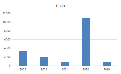
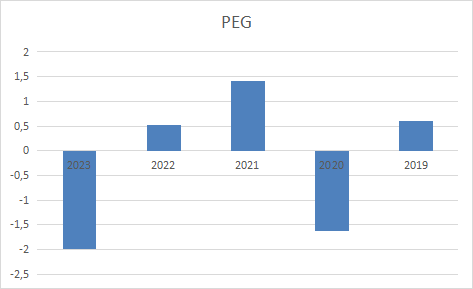
- NVDA bar chart visuals of the Excel spreadsheet fundamentalsnvda.xlsx
       Rows:

Mkt Cap
Debt to Equity
Debt to Assets
Revenue per Share
NI per Share
Revenue
Gross Profit
R&D Expenses
Op Expenses
Op Income
Net Income
Cash
Inventory
Cur Assets
LT Assets
Int Assets
Total Assets
Cur Liab
LT Debt
LT Liab
Total Liab
SH Equity
CF Operations
CF Investing
CF Financing
CAPEX
FCF
Dividends Paid
Gross Profit Margin
Op Margin
Int Coverage
Net Profit Margin
Dividend Yield
Current Ratio
Operating Cycle
Days of AP Outstanding
Cash Conversion Cycle
ROA
ROE
ROCE
PE
PS
PB
Price To FCF
PEG
EPS
         Columns:
2023	2022	2021	2020	2019	CAGR	2023 growth	2022 growth	2021 growth

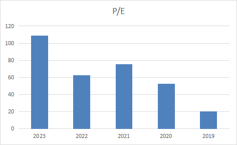


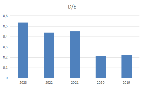
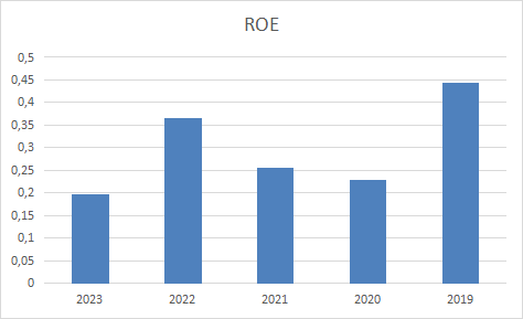

- Overall NVDA gets a fundamental rating of 7 out of 10.
- The Altman-Z score of NVDA (29.91) is better than 95.24% of its industry peers.
- NVDA has a better Debt to FCF ratio (0.94) than 77.14% of its industry peers.
- NVDA‘s Current ratio of 2.79 is in line compared to the rest of the industry. NVDA outperforms 41.90% of its industry peers.
- In the last year, the EPS has been growing by 20.41%, which is quite impressive.
- The EPS will grow by 54.68% on average per year.
- NVDA is valuated quite expensively with a Price/Earnings ratio of 77.68.
- The average S&P500 Price/Earnings ratio is at 22.86. NVDA is valued rather expensively when compared to this.
- 68.57% of the companies in the same industry are cheaper than NVDA, based on the Enterprise Value to EBITDA ratio.
- The excellent profitability rating of NVDA may justify a higher PE ratio.
- NVDA has a yearly dividend return of 0.04%, which is pretty low.
- The dividend of NVDA has a limited annual growth rate of 2.26%.
Indian Dividend Stock Portfolio 3
- In this section, we will use the CAPM model to examine the risk/return ratio of Indian dividend stocks listed in NIFTY 50 (a benchmark Indian stock market index).
- Let’s set the working directory YOURPATH
import os
os.chdir('YOURPATH')
os. getcwd()
- Importing the key libraries
import numpy as np
import pandas as pd
import matplotlib.pyplot as plt
from nsepy import get_history as gh
from datetime import date
- Defining the time interval and tickers (initial configuration)
start_date = date(2018,2,2)
end_date = date(2023,2,2)
tickers = ['TATAMOTORS','DABUR', 'ICICIBANK','WIPRO','INFY']
- Loading the stock data, creating portfolio 3 and calculating the daily returns
def load_stock_data(start_date, end_date, ticker):
    df = pd.DataFrame()
    for i in range(len(ticker)):
        data = gh(symbol=ticker[i],start= start_date, end=end_date)[['Symbol','Close']]
        data.rename(columns={'Close':data['Symbol'][0]},inplace=True)
        data.drop(['Symbol'], axis=1,inplace=True)
        if i == 0:
            df = data
        if i != 0:
            df = df.join(data)

    return df
# Loading the stock data in the tickers from NSEPY data for specified period
df_stock = load_stock_data(start_date, end_date, tickers)

# Loading the NIFTY data for specified period
df_nifty = gh(symbol = 'NIFTY',start = date(2018,2,2), end = date(2023,2,2), index= True)[['Close']]
df_nifty.rename(columns = {'Close':'NIFTY'}, inplace = True)
df_port = pd.concat([df_stock, df_nifty], axis = 1)

# Calculating daily returns
df_returns = df_port.pct_change().dropna().reset_index()
df_port 5 selected rows:

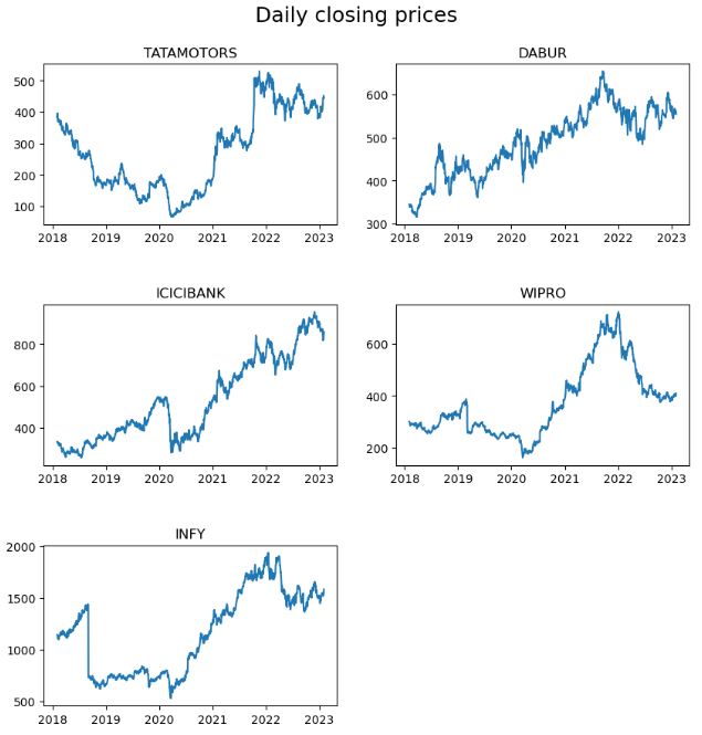
- Plotting the stock daily closing prices
plt.figure(figsize=(10, 10))
plt.subplots_adjust(hspace=0.5)
plt.suptitle("Daily closing prices", fontsize=18, y=0.95)
for n, ticker in enumerate(tickers):
    ax = plt.subplot(3, 2, n + 1)
    df_stock[ticker].plot(ax= ax)
    ax.set_title(ticker.upper())
    ax.set_xlabel("")
plt.savefig('capmprice.png', transparent=True)
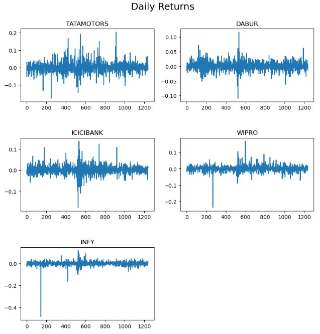
- Plotting daily returns
plt.figure(figsize=(10, 10))
plt.subplots_adjust(hspace=0.5)
plt.suptitle("Daily Returns", fontsize=18, y=0.95)
for n, ticker in enumerate(tickers):
    ax = plt.subplot(3, 2, n + 1)
    df_returns[ticker].plot(ax= ax)
    ax.set_title(ticker.upper())
    ax.set_xlabel("")
plt.savefig('capmreturns.png', transparent=True)
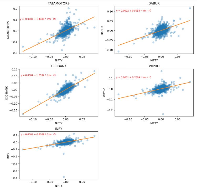
- Fitting a regression line stock vs NIFTY to estimate beta and alpha
beta = []
alpha = []

for i in df_returns.columns:
  if i != 'Date' and i != 'NIFTY':
    df_returns.plot(kind = 'scatter', x = 'NIFTY', y = i)
    b, a = np.polyfit(df_returns['NIFTY'], df_returns[i], 1)
    plt.plot(df_returns['NIFTY'], b * df_returns['NIFTY'] + a, '-', color = 'r')
    beta.append(b)
    alpha.append(a)
- Plotting the linear regression lines
plt.figure(figsize=(10, 10))
plt.subplots_adjust(hspace=0.5)
plt.suptitle("", fontsize=18, y=0.95)
for n, ticker  in enumerate(tickers):
    ax = plt.subplot(3, 2, n + 1)
    plt.plot(df_returns['NIFTY'], df_returns[ticker], 'o', alpha = 0.3)
    b, a = np.polyfit(df_returns['NIFTY'], df_returns[ticker], 1)
    plt.plot(df_returns['NIFTY'], b * df_returns['NIFTY'] + a, '-')
    ax.set_title(ticker.upper())
    ax.set_xlabel('NIFTY')
    ax.set_ylabel(ticker)
    plt.tight_layout()
    plt.text(-0.03, 0.1, f'y = {round(a, 4)} + {round(b, 4)} * (rm - rf)',
         horizontalalignment='right',
         size='small', color='red')
plt.savefig('capmreg.png', transparent=True)
- Calculating CAPM-based expected returns
ER = []
rf = 0
rm = df_returns['NIFTY'].mean() * 252
print(f'Market return is {rm}%')
for i, b in enumerate(beta):
    ER_tmp = rf + (b * (rf - rm)) * 100
    ER.append(ER_tmp)
    print(f'Expected return based on CAPM for {tickers[i]} is  {round(ER_tmp,2)} %')

Market return is 0.11933857013790888%
Expected return based on CAPM for TATAMOTORS is  -17.29 %
Expected return based on CAPM for DABUR is  -7.1 %
Expected return based on CAPM for ICICIBANK is  -16.22 %
Expected return based on CAPM for WIPRO is  -8.36 %
Expected return based on CAPM for INFY is  -9.8 %
- Assigning portfolio weights and calculating the expected portfolio return
portfolio_weights = 1/len(tickers) * np.ones(len(tickers))
ER_portfolio = sum(ER * portfolio_weights)
print(f'Portfolio expected return is {round(ER_portfolio,2)} %')

Portfolio expected return is -11.76 %

print(portfolio_weights)

[0.2 0.2 0.2 0.2 0.2]

print(alpha)

[-8.918248566266388e-05, 0.00022239414251699533, 0.00035961301093695073, 0.0001049024358274514, 0.0001856998089880721]

print(beta)

[1.4488042079008974, 0.5953470049512081, 1.3592314779510428, 0.7008874168511913, 0.8208594560575715]
- Computing the Security market Line (SML)
sml_beta = pd.DataFrame(beta,columns =['beta'])
sml_returns = pd.DataFrame(ER,columns =['ER'])
sml = pd.concat([sml_beta, sml_returns], axis = 1)

fig, ax = plt.subplots(figsize=(8, 5))
plt.plot(sml['beta'], sml['ER'])


ax.set_title('Security Market Line')
ax.set_xlabel('Beta')
ax.set_ylabel('Expected Returns')

- Let’s optimize portfolio 3 in terms of stock VAR
# Import libraries

import numpy as np
import pandas as pd
import warnings
import matplotlib.pyplot as plt
import matplotlib.patches as mpatches
from statistics import NormalDist
import statistics
import seaborn as sns
from datetime import date
from tabulate import tabulate
from nsepy import get_history as gh
from mplcursors import cursor
plt.style.use('fivethirtyeight')
warnings.filterwarnings('ignore')
pd.set_option('display.max_rows', None)
# Define configurations
initial_investment: int = 100000
start_date = date(2022,2,2)
# end_date = date.today()
end_date = date(2023,2,2)
stocksymbols = ['TATAMOTORS','DABUR', 'ICICIBANK','WIPRO','INFY']
weights = np.array([0.4, 0.2, 0.1, 0.1, 0.2])
# Data loading and computing Return-VAR

def load_stock_data(start_date, end_date, investment: int, ticker: str):
    df = pd.DataFrame()
    for i in range(len(ticker)):
        data = gh(symbol=ticker[i],start= start_date, end=end_date)[['Symbol','Close']]
        data.rename(columns={'Close':data['Symbol'][0]},inplace=True)
        data.drop(['Symbol'], axis=1,inplace=True)
        if i == 0:
            df = data
        if i != 0:
            df = df.join(data)

    return df


df_stockPrice = load_stock_data(start_date, end_date, initial_investment, stocksymbols)
df_returns = df_stockPrice.pct_change().dropna()


portfolio = (weights * df_returns.values).sum(axis=1)
port_var = np.percentile(portfolio, 5, interpolation = 'lower')
port_var

-0.022599923823150847
- Bootstrap (basic) simulation
def sim_portfolio(weights):
    # port_stdev = np.sqrt(weights.T.dot(cov_matrix).dot(weights))
    # return port_stdev
    tmp_pp = (weights * df_returns.values).sum(axis=1)
    var_sim_port = np.percentile(tmp_pp, 5, interpolation = 'lower')
    return var_sim_port


port_returns = []
port_volatility = []
port_weights = []

num_assets = len(stocksymbols)
num_portfolios = 10000
np.random.seed(1357)
for port in range(num_portfolios):
    weights = np.random.random(num_assets)
    weights = weights/sum(weights)
    port_weights.append(weights)

    df_wts_returns = df_returns.mean().dot(weights)
    port_returns.append(df_wts_returns*100)

    var_port_95 = sim_portfolio(weights)
    port_volatility.append(var_port_95)
port_weights = [[round(wt[0],5), round(wt[1],5), round(wt[2],5),round(wt[3],5),round(wt[4],5)] for wt  in port_weights]
dff = {'Returns': port_returns, 'Risk': port_volatility, 'Weights': port_weights}
df_risk = pd.DataFrame(dff)
df_risk.info()
<class 'pandas.core.frame.DataFrame'>
RangeIndex: 10000 entries, 0 to 9999
Data columns (total 3 columns):
 #   Column   Non-Null Count  Dtype
---  ------   --------------  -----
 0   Returns  10000 non-null  float64
 1   Risk     10000 non-null  float64
 2   Weights  10000 non-null  object
dtypes: float64(2), object(1)
memory usage: 234.5+ KB
df_risk[(df_risk['Risk'] > -0.02) & (df_risk['Returns'] > 0.01)]
        Returns	       Risk	    Weights
997	    0.010809	-0.019637	[0.15549, 0.30334, 0.48221, 0.01111, 0.04785]
1095	0.011785	-0.018679	[0.02925, 0.11915, 0.65296, 0.02588, 0.17276]
4526	0.010994	-0.019101	[0.08346, 0.13514, 0.6049, 0.01273, 0.16377]
5457	0.011373	-0.019397	[0.12779, 0.31885, 0.47465, 0.00504, 0.07367]
6658	0.010704	-0.019479	[0.12018, 0.32579, 0.50025, 0.0314, 0.02238]
8159	0.012759	-0.019898	[0.08113, 0.2709, 0.54323, 0.01251, 0.09222]
9963	0.010442	-0.019877	[0.0012, 0.42383, 0.44869, 0.03354, 0.09274]
df_risk['Risk'].max()
-0.016895038141191226

df_risk['Risk'].min()
-0.03263339159510597

df_risk['Returns'].max()
0.017049520522481834

df_risk['Returns'].min()
-0.09880198482191363
- Selecting new weights for min/max returns and risk
max_risk = df_risk.iloc[df_risk['Risk'].idxmin()]
max_risk[0]
max_risk[1]
max_risk[2]

[0.82771, 0.00729, 0.14223, 0.0197, 0.00307]

min_risk = df_risk.iloc[df_risk['Risk'].idxmax()]
min_risk[0]
min_risk[1]
min_risk[2]

[0.05294, 0.34003, 0.30989, 0.18632, 0.11082]

max_returns = df_risk.iloc[df_risk['Returns'].idxmax()]
max_returns[0]
max_returns[1]
max_returns[2]

[0.03087, 0.3918, 0.52679, 0.00689, 0.04365]

min_returns = df_risk.iloc[df_risk['Returns'].idxmin()]
min_returns[0]
min_returns[1]
min_returns[2]

[0.00399, 0.04691, 0.09405, 0.74185, 0.1132]

# Portfolio VAR for the basic simulation
port_var_basic_sim = sim_portfolio(min_risk[2])
port_var_basic_sim

-0.01689496173724531
- Selecting new weights using the decay factor
def var_weighted_decay_factor(weights):

    returns = df_returns.copy()
    returns['Stock'] = (weights * returns.values).sum(axis=1)
    # returns = returns['Stock']
    decay_factor = 0.5 #we’re picking this arbitrarily
    n = len(returns)
    wts = [(decay_factor**(i-1) * (1-decay_factor))/(1-decay_factor**n) for i in range(1, n+1)]

    #Need to reverse the PnL to put recent returns on top
    returns_recent_first = returns[::-1]
    weights_dict = {'Returns':returns_recent_first, 'Weights':wts}

    wts_returns = pd.DataFrame(returns_recent_first['Stock'])
    wts_returns['wts'] = wts

    sort_wts = wts_returns.sort_values(by='Stock')
    sort_wts['Cumulative'] = sort_wts.wts.cumsum()
    sort_wts

    #Find where cumulative (percentile) hits 0.05
    sort_wts = sort_wts.reset_index()
    idx = sort_wts[sort_wts.Cumulative <= 0.05].Stock.idxmax()
    sort_wts.filter(items = [idx], axis = 0)


    xp = sort_wts.loc[idx:idx+1, 'Cumulative'].values
    fp = sort_wts.loc[idx:idx+1, 'Stock'].values
    var_decay = np.interp(0.05, xp, fp)

    print(f'The VAR of stock using decay factor is {var_decay} ')
    return var_decay


port_var_decay = var_weighted_decay_factor(weights)

The VAR of stock using decay factor is 0.002261753934614717
- Plotting the financial portfolio in Excel

Others: DABUR, WIPRO, INFY
- Plotting price trends
def plot_price_trends():
    fig, ax = plt.subplots(figsize=(15,8))
    for i in df_stockPrice.columns.values :
        ax.plot(df_stockPrice[i], label = i)
    ax.set_title("Portfolio Close Price History")
    ax.set_xlabel('Date', fontsize=18)
    ax.set_ylabel('Close Price INR (₨)' , fontsize=18)
    ax.legend(df_stockPrice.columns.values , loc = 'upper right')
    plt.show(fig)


plot_price_trends()

- Plotting daily simple returns
def plot_daily_return_trends():

    print('Daily simple returns')
    fig, ax = plt.subplots(figsize=(15,8))
    for i in df_returns.columns.values :
        ax.plot(df_returns[i], lw =2 ,label = i)

    ax.legend( loc = 'upper right' , fontsize =10)
    ax.set_title('Volatility in Daily simple returns ')
    ax.set_xlabel('Date')
    ax.set_ylabel('Daily simple returns')
    plt.show(fig)

    print('Average Daily returns(%) of stocks in your portfolio')
    Avg_daily = df_returns.mean()
    print(Avg_daily*100)

    print('Annualized Standard Deviation (Volatality(%), 252 trading days) of individual stocks in your portfolio on the basis of daily simple returns.')
    print(df_returns.std() * np.sqrt(252) * 100)

    print('Return per unit of risk')
    Avg_daily / (df_returns.std() * np.sqrt(252)) *100


plot_daily_return_trends()
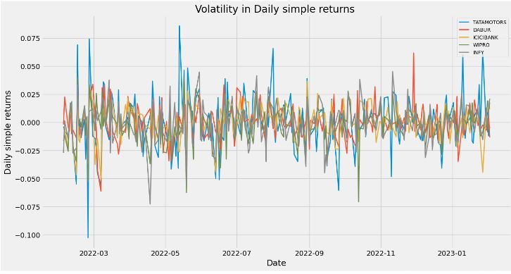
Average Daily returns(%) of stocks in your portfolio
TATAMOTORS   -0.026735
DABUR         0.008902
ICICIBANK     0.031856
WIPRO        -0.132460
INFY         -0.033956
dtype: float64
Annualized Standard Deviation (Volatility(%), 252 trading days) of individual stocks in your portfolio on the basis of daily simple returns.
TATAMOTORS    35.808329
DABUR         23.661057
ICICIBANK     23.140343
WIPRO         25.312352
INFY          27.060286
dtype: float64
Return per unit of risk
- Plotting daily cumulative simple returns
def plot_daily_cumulative_returns():

    daily_cummulative_simple_return =(df_returns+1).cumprod()
    daily_cummulative_simple_return
    #visualize the daily cummulative simple return
    print('Cummulative Returns')
    fig, ax = plt.subplots(figsize=(18,8))

    for i in daily_cummulative_simple_return.columns.values :
        ax.plot(daily_cummulative_simple_return[i], lw =2 ,label = i)

    ax.legend( loc = 'upper left' , fontsize =10)
    ax.set_title('Daily Cumulative Simple returns/growth of investment')
    ax.set_xlabel('Date')
    ax.set_ylabel('Growth of ₨ 1 investment')
    cursor(hover=True)
    plt.show()


plot_daily_cumulative_returns()
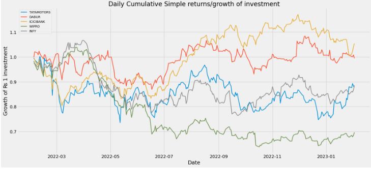
- Plotting the histogram of weighted simulated returns
weights = [0.05294, 0.34003, 0.30989, 0.18632, 0.11082]
ddf = df_returns.copy()
ddf['Stock'] = (weights * ddf.values).sum(axis=1)

fig, ax = plt.subplots(figsize=(10, 5))
ax.grid(False)
sns.histplot(ddf['Stock'],color = 'blue',alpha = .2,bins = 50,
                edgecolor = "black", kde = True)
plt.text(port_var_basic_sim, 17, f'VAR {round(port_var_basic_sim, 4)} @ 5%',
         horizontalalignment='right',
         size='small', color='navy')
left, bottom, width, height = (port_var_basic_sim, 0, -5, 550)
rect=mpatches.Rectangle((left,bottom),width,height,
                        fill=True,
                        color="red",
                        alpha=0.2,
                        facecolor="red",
                       linewidth=2)

ax.set_title('Distribution of simulated returns')
ax.set_xlabel('Weighed stock returns')
ax.set_ylabel('Frequency')

plt.gca().add_patch(rect)
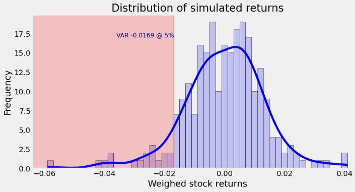
- Let’s examine portfolio optimization using max Sharpe Ratio
import numpy as np
import pandas as pd
import warnings
import matplotlib.pyplot as plt
import matplotlib.patches as mpatches
from statistics import NormalDist
import statistics
import seaborn as sns
from datetime import date
from tabulate import tabulate
from nsepy import get_history as gh
from mplcursors import cursor
plt.style.use('fivethirtyeight') #setting matplotlib style
warnings.filterwarnings('ignore')
pd.set_option('display.max_rows', None)


##################################################################
# Define configurations
##################################################################
initial_investment: int = 100000
start_date = date(2022,2,2)
# end_date = date.today()
end_date = date(2023,2,2)
# stocksymbols = ['TATAMOTORS','DABUR', 'ICICIBANK','WIPRO','INFY']
# weights = np.array([0.4, 0.2, 0.1, 0.1, 0.2])

stocksymbols = ['AXISBANK', 'HDFCBANK', 'ICICIBANK', 'KOTAKBANK', 'SBIN']
weights = np.array([0.2, 0.2, 0.2, 0.2, 0.2])


##################################################################
# Data loading for given time period
##################################################################

def load_stock_data(start_date, end_date, investment: int, ticker: str):
    df = pd.DataFrame()
    for i in range(len(ticker)):
        data = gh(symbol=ticker[i],start= start_date, end=end_date)[['Symbol','Close']]
        data.rename(columns={'Close':data['Symbol'][0]},inplace=True)
        data.drop(['Symbol'], axis=1,inplace=True)
        if i == 0:
            df = data
        if i != 0:
            df = df.join(data)

    return df


df_stockPrice = load_stock_data(start_date, end_date, initial_investment, stocksymbols)
df_returns = df_stockPrice.pct_change().dropna()


df_returns['Portfolio'] = (weights * df_returns.values).sum(axis=1)
df_returns.head(3)

# Average daily return
df_returns['Portfolio'].mean()

# Standard deviation of the portfolio
df_returns['Portfolio'].std()
df_returns['Portfolio'].plot(kind='kde')


# Sharpe ratio
sharpe_ratio = df_returns['Portfolio'].mean() / df_returns['Portfolio'].std()
Distribution of portfolio average daily return STD:

- Histograms of stock returns
df_returns.hist(bins=100,figsize=(12,6))
plt.tight_layout()
plt.savefig('hist_banks.png', transparent=True)

- Stock price trends
fig, ax = plt.subplots(figsize=(15,8))
for i in df_stockPrice.columns.values :
    ax.plot(df_stockPrice[i], label = i)
ax.set_title("Portfolio Close Price History")
ax.set_xlabel('Date', fontsize=18)
ax.set_ylabel('Close Price INR (₨)' , fontsize=18)
ax.legend(df_stockPrice.columns.values , loc = 'upper right')
plt.show(fig)

- Stock price daily cumulative simple return trends
daily_cummulative_simple_return =(df_returns+1).cumprod()
fig, ax = plt.subplots(figsize=(18,8))
for i in daily_cummulative_simple_return.columns.values :
    ax.plot(daily_cummulative_simple_return[i], lw =2 ,label = i)

ax.legend( loc = 'upper left' , fontsize =10)
ax.set_title('Daily Cumulative Simple returns/growth of investment')
ax.set_xlabel('Date')
ax.set_ylabel('Growth of ₨ 1 investment')
cursor(hover=True)

- Sharpe-based simple portfolio simulation
def sim_portfolio(weights):
    # port_stdev = np.sqrt(weights.T.dot(cov_matrix).dot(weights))
    # return port_stdev
    port_mean = (weights * df_returns.values).sum(axis=1)
    # Annualized mean
    port_mean = port_mean * 252
    port_sd = np.sqrt(weights.T.dot(df_returns.cov() * 252 ).dot(weights))


    port_var = np.percentile(port_mean/252, 5, interpolation = 'lower')
    port_var_95.append(port_var)

    port_volatility.append(port_sd)
    mc_sim_sr = (port_mean.mean() / port_sd)

    return mc_sim_sr


port_var_95 = []
port_returns = []
port_volatility = []
port_weights = []
sharpe_ratio = []

num_assets = len(stocksymbols)+1
num_portfolios = 25000
np.random.seed(1357)

for port in range(num_portfolios):
    weights = np.random.random(num_assets)
    weights = weights/sum(weights)
    port_weights.append(weights)
    df_wts_returns = df_returns.mean().dot(weights)
    port_returns.append(df_wts_returns*100)
mc_sim_sr = sim_portfolio(weights)
sharpe_ratio.append(mc_sim_sr)
print (df_returns.mean())

AXISBANK     0.000463
HDFCBANK     0.000314
ICICIBANK    0.000319
KOTAKBANK   -0.000279
SBIN         0.000052
Portfolio    0.000174
dtype: float64
print(sharpe_ratio)

[0.31098709022009735]
port_weights = [[round(wt[0],5), round(wt[1],5), round(wt[2],5),round(wt[3],5),round(wt[4],5)] for wt in port_weights]
dff = {'Returns': port_returns, 'Risk': port_volatility, 'Sharpe Ratio': sharpe_ratio, 'Weights': port_weights, 'Port_var_95':port_var_95}
dff1 = {'Returns': port_returns, 'Weights': port_weights}
df_risk = pd.DataFrame(dff1)
df_risk.tail(5)

        Returns	              Weights
24995	0.032083	[0.34585, 0.16636, 0.21691, 0.00384, 0.04906]
24996	0.016130	[0.1135, 0.24677, 0.1266, 0.15215, 0.24069]
24997	0.011851	[0.17142, 0.05479, 0.1281, 0.22531, 0.23796]
24998	0.017672	[0.2083, 0.22489, 0.15547, 0.21647, 0.10923]
24999	0.025926	[0.18055, 0.20231, 0.25359, 0.00945, 0.2262]
# Sharpe ratio
sharpe_ratio = df_returns['Portfolio'].mean() / df_returns['Portfolio'].std()

print(sharpe_ratio)
0.013485073404367168
- Calculate and plot portfolio risk using VAR
ddf_risk = df_returns.copy()
ddf_risk['Stock'] = (weights * ddf_risk.values).sum(axis=1)
ddf_risk.head(5)
ddf_risk['Stock'].max()

port_var_mean_95 = statistics.mean(port_var_95)

fig, ax = plt.subplots(figsize=(10, 5))
sns.histplot(ddf_risk['Stock'],color = 'blue',alpha = .2,bins = 50,
                edgecolor = "black", kde = True)
plt.xlabel('Volatility')
plt.ylabel('Stock Return')
plt.text(port_var_mean_95, 23, f'VAR {round(port_var_mean_95, 4)} @ 5%',
         horizontalalignment='right',
         size='small', color='navy')
left, bottom, width, height = (port_var_mean_95, 0, -5, 1750)
rect=mpatches.Rectangle((left,bottom),width,height,
                        fill=True,
                        color="red",
                        alpha=0.2,
                        facecolor="red",
                       linewidth=2)
plt.gca().add_patch(rect)
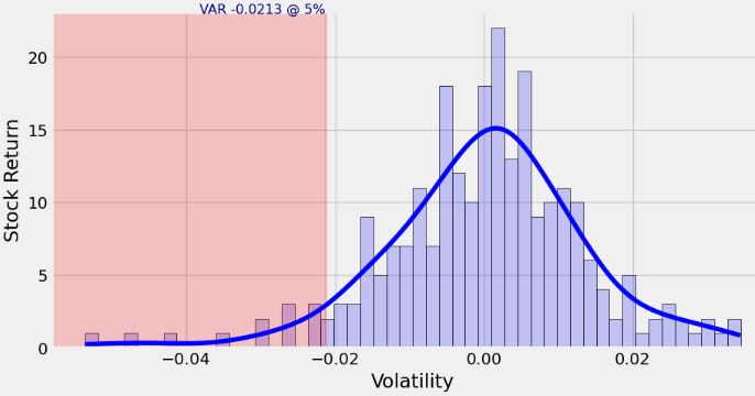
- Stochastic Portfolio Optimization using the Stock Risk Class in Appendix A
obj_var = StockRisk(startdate, end_date, initial_investment, stocksymbols, iterations)
obj_var.var_historical()
╒════════════════╤═════════╤══════════════════════╤═════════╕
│                │  Mean   │  Standard Deviation  │  VaR %  │
╞════════════════╪═════════╪══════════════════════╪═════════╡
│ ['TATAMOTORS'] │ -0.0003 │        0.0226        │ -0.0393 │
╘════════════════╧═════════╧══════════════════════╧═════════╛
-0.039306077884265433
-0.039306077884265433
obj_var.var_bootstrap()

The Bootstrap VaR measure is -0.03692893950287173
-0.03692893950287173
obj_var.var_weighted_decay_factor()

The VAR of stock using decay factor is -0.012218757045694294
-0.012218757045694294
obj_var.var_monte_carlo()

The mean Monte Carlo VaR is -0.03721525740992629
-0.03721525740992629
obj_var.show_summary()

╒════════════════╤═════════╤══════════════════════╤═════════╕
│                │  Mean   │  Standard Deviation  │  VaR %  │
╞════════════════╪═════════╪══════════════════════╪═════════╡
│ ['TATAMOTORS'] │ -0.0003 │        0.0226        │ -0.0393 │
╘════════════════╧═════════╧══════════════════════╧═════════╛
-0.039306077884265433
The Bootstrap VaR measure is -0.03677416902540935
The VAR of stock using decay factor is -0.012218757045694294
The mean Monte Carlo VaR is -0.037324210445353556

╒════════════════╤══════════════╤═════════════╤═════════╤═══════════════╕
│                │  Historical  │  Bootstrap  │  Decay  │  Monte Carlo  │
╞════════════════╪══════════════╪═════════════╪═════════╪═══════════════╡
│ ['TATAMOTORS'] │   -0.0393    │   -0.0368   │ -0.0122 │    -0.0373    │
╘════════════════╧══════════════╧═════════════╧═════════╧═══════════════╛
obj_var.plot_stock_returns_shaded('historical')

╒════════════════╤═════════╤══════════════════════╤═════════╕
│                │  Mean   │  Standard Deviation  │  VaR %  │
╞════════════════╪═════════╪══════════════════════╪═════════╡
│ ['TATAMOTORS'] │ -0.0003 │        0.0226        │ -0.0393 │
╘════════════════╧═════════╧══════════════════════╧═════════╛
-0.039306077884265433

obj_var.plot_stock_returns_shaded('bootstrap')
The Bootstrap VaR measure is -0.03675094394004405
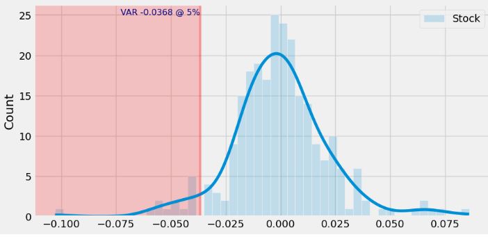
obj_var.plot_stock_returns_shaded('decay')
The VAR of stock using decay factor is -0.012218757045694294

obj_var.plot_stock_returns_shaded('monte_carlo')
The mean Monte Carlo VaR is -0.03722746593892233
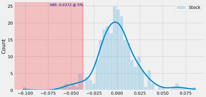
BTC-USD Price Analysis and Forecasting
- Let’s discuss the BTC-USD price prediction using FB Prophet
- Setting the working directory YOURPATH
import os
os.chdir('YOURPATH')
os. getcwd()
- Importing the key libraries
import pandas as pd
import plotly.express as px
import requests
import numpy as np
import matplotlib.pyplot as plt
from math import floor
from termcolor import colored as cl

plt.rcParams['figure.figsize'] = (20, 10)
plt.style.use('fivethirtyeight')
- Reading input BTC-USD data with start_date = ‘2021-01-01’
def get_crypto_price(symbol, exchange, start_date = None):
    api_key = 'YOUR API KEY'
    api_url = f'https://www.alphavantage.co/query?function=DIGITAL_CURRENCY_DAILY&symbol={symbol}&market={exchange}&apikey={api_key}'
    raw_df = requests.get(api_url).json()
    df = pd.DataFrame(raw_df['Time Series (Digital Currency Daily)']).T
    df = df.rename(columns = {'1a. open (USD)': 'Open', '2a. high (USD)': 'High', '3a. low (USD)': 'Low', '4a. close (USD)': 'Close', '5. volume': 'Volume'})
    for i in df.columns:
        df[i] = df[i].astype(float)
    df.index = pd.to_datetime(df.index)
    df = df.iloc[::-1].drop(['1b. open (USD)', '2b. high (USD)', '3b. low (USD)', '4b. close (USD)', '6. market cap (USD)'], axis = 1)
    if start_date:
        df = df[df.index >= start_date]
    return df

btc = get_crypto_price(symbol = 'BTC', exchange = 'USD', start_date = '2021-01-01')
df=btc.copy()
df.tail()

print(df.info())
print(df.describe())
<class 'pandas.core.frame.DataFrame'>
DatetimeIndex: 1000 entries, 2021-02-04 to 2023-10-31
Data columns (total 5 columns):
 #   Column  Non-Null Count  Dtype
---  ------  --------------  -----
 0   Open    1000 non-null   float64
 1   High    1000 non-null   float64
 2   Low     1000 non-null   float64
 3   Close   1000 non-null   float64
 4   Volume  1000 non-null   float64
dtypes: float64(5)
memory usage: 46.9 KB
None
               Open         High           Low         Close         Volume
count   1000.000000   1000.00000   1000.000000   1000.000000    1000.000000
mean   34522.491010  35369.12544  33583.302750  34519.529780  109613.282187
std    13032.574677  13435.22670  12543.179668  13032.368197  112947.462568
min    15781.290000  16315.00000  15476.000000  15781.290000     740.906180
25%    23545.567500  24219.43000  23109.972500  23545.567500   39087.027808
50%    30287.075000  30743.66000  29713.680000  30287.075000   61984.789660
75%    44405.345000  45804.71750  43017.272500  44404.550000  141226.111672
max    67525.820000  69000.00000  66222.400000  67525.830000  760705.362783
df.reset_index(inplace=True)
df.rename(columns={'index': 'Date'}, inplace=True)
px.area(df, x='Date', y='Close')
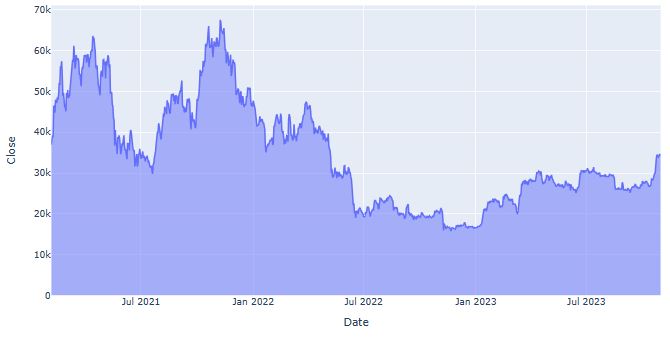
px.box(df, y='Close')
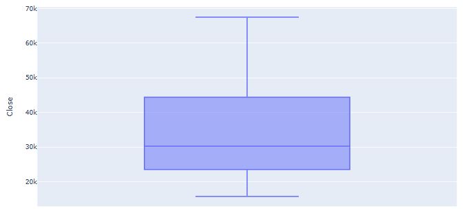
### Boxcox transformation
from statsmodels.base.transform import BoxCox

bc= BoxCox()
df["Close"], lmbda =bc.transform_boxcox(df["Close"])
## Making data Prophet compliant
data= df[["Date", "Close"]]
data.columns=["ds", "y"]
## Creating model parameters
model_param ={
    "daily_seasonality": False,
    "weekly_seasonality":False,
    "yearly_seasonality":True,
    "seasonality_mode": "multiplicative",
    "growth": "logistic"
}
# Import Prophet
from prophet import Prophet
model = Prophet(**model_param)
data['cap']= data["y"].max() + data["y"].std() * 0.05
# Setting a cap or upper limit for the forecast as we are using logistics growth
# The cap will be maximum value of target variable plus 5% of std.

model.fit(data)

# Create future dataframe
future= model.make_future_dataframe(periods=365)
#future= model.make_future_dataframe(periods=60)
future['cap'] = data['cap'].max()

forecast= model.predict(future)
model.plot_components(forecast);

model.plot(forecast);# block dots are actual values and blue dots are forecast

## Adding parameters and seasonality and events

from IPython.core.display import display, HTML
display(HTML("<style>div.output_scroll { height: 144em; }</style>"))

model = Prophet(**model_param)

model= model.add_seasonality(name="monthly", period=30, fourier_order=10)
model= model.add_seasonality(name="quarterly", period=92.25, fourier_order=10)

model.add_country_holidays("US")

model.fit(data)

# Create future dataframe
future= model.make_future_dataframe(periods=365)
future['cap'] = data['cap'].max()

forecast= model.predict(future)
model.plot_components(forecast);
model.plot(forecast);


## Hyper parameter Tuning
import itertools
import numpy as np
from prophet.diagnostics import cross_validation, performance_metrics


param_grid={
    "daily_seasonality": [False],
    "weekly_seasonality":[False],
    "yearly_seasonality":[True],
    "growth": ["logistic"],
    'changepoint_prior_scale': [0.001, 0.01, 0.1, 0.5], # to give higher value to prior trend
    'seasonality_prior_scale': [0.01, 0.1, 1.0, 10.0] # to control the flexibility of seasonality components
}

# Generate all combination of parameters
all_params= [
            dict(zip(param_grid.keys(), v))
            for v in itertools.product(*param_grid.values())
]

#print(all_params)
rmses= list ()

# go through each combinations
for params in all_params:
    m= Prophet(**params)

#    m= m.add_seasonality(name= 'monthly', period=30, fourier_order=5)
#    m= m.add_seasonality(name= "quarterly", period= 92.25, fourier_order= 10)

    m= m.add_seasonality(name= 'monthly', period=15, fourier_order=5)
    m= m.add_seasonality(name= "quarterly", period= 30, fourier_order= 10)
    m.add_country_holidays(country_name="US")

    m.fit(data)

#    df_cv= cross_validation(m, initial="730 days", period="365 days", horizon="365 days")

    df_cv= cross_validation(m, initial="365 days", period="30 days", horizon="365 days")

    df_p= performance_metrics(df_cv, rolling_window=1)

    rmses.append(df_p['rmse'].values[0])

# find teh best parameters
best_params = all_params[np.argmin(rmses)]

print("\n The best parameters are:", best_params)
The best parameters are: {'daily_seasonality': False, 'weekly_seasonality': False, 'yearly_seasonality': True, 'growth': 'logistic', 'changepoint_prior_scale': 0.001, 'seasonality_prior_scale': 0.1}
#forecast.head()
forecast["yhat"]=bc.untransform_boxcox(x=forecast["yhat"], lmbda=lmbda)
forecast["yhat_lower"]=bc.untransform_boxcox(x=forecast["yhat_lower"], lmbda=lmbda)
forecast["yhat_upper"]=bc.untransform_boxcox(x=forecast["yhat_upper"], lmbda=lmbda)
forecast.plot(x="ds", y=["yhat_lower", "yhat", "yhat_upper"])

- Referring to the earlier studies, let’s consider BTC-USD Price forecasting with deep learning algorithms, viz. LSTM and GRU.
- Importing the key libraries
import warnings
warnings.filterwarnings("ignore")

import numpy as np
import pandas as pd
import statsmodels.api as sm
from scipy import stats
from sklearn.metrics import mean_squared_error
from math import sqrt
from random import randint
from keras.models import Sequential
from keras.layers import Dense
from keras.layers import LSTM
from keras.layers import GRU
from keras.callbacks import EarlyStopping
from keras import initializers
from matplotlib import pyplot
from datetime import datetime
from matplotlib import pyplot as plt
import plotly.offline as py
import plotly.graph_objs as go
py.init_notebook_mode(connected=True)
%matplotlib inline
- Reading the input BTC-USD time series data
import pandas as pd
import yfinance as yf
import datetime
from datetime import date, timedelta
today = date.today()

d1 = today.strftime("%Y-%m-%d")
end_date = d1
d2 = date.today() - timedelta(days=730)
d2 = d2.strftime("%Y-%m-%d")
start_date = d2

data = yf.download('BTC-USD',
                      start=start_date,
                      end=end_date,
                      progress=False)
data["Date"] = data.index
data = data[["Date", "Open", "High", "Low", "Close", "Adj Close", "Volume"]]
data.reset_index(drop=True, inplace=True)
print(data.tail())
         Date          Open          High           Low         Close  \
725 2023-10-26  34504.289062  34832.910156  33762.324219  34156.648438
726 2023-10-27  34156.500000  34238.210938  33416.886719  33909.800781
727 2023-10-28  33907.722656  34399.390625  33874.804688  34089.574219
728 2023-10-29  34089.371094  34743.261719  33947.566406  34538.480469
729 2023-10-30  34531.742188  34843.933594  34110.972656  34502.363281

        Adj Close       Volume
725  34156.648438  19427195376
726  33909.800781  16418032871
727  34089.574219  10160330825
728  34538.480469  11160323986
729  34502.363281  17184860315
- Train/test data preparation
data.isnull().values.any()
False
group = data.groupby('Date')
Daily_Price = group['Close'].mean()

Daily_Price.tail()

Date
2023-10-26    34156.648438
2023-10-27    33909.800781
2023-10-28    34089.574219
2023-10-29    34538.480469
2023-10-30    34502.363281
Name: Close, dtype: float64
from datetime import date
d0 = date(2022, 1, 15)
d1 = date(2023, 10, 30)
delta = d1 - d0
days_look = delta.days + 1
print(days_look)

654
d0 = date(2022, 12, 15)
d1 = date(2023, 10, 30)
delta = d1 - d0
days_from_train = delta.days + 1
print(days_from_train)

320
d0 = date(2023, 2, 5)
d1 = date(2023, 10, 30)
delta = d1 - d0
days_from_end = delta.days + 1
print(days_from_end)

268
df_train= Daily_Price[len(Daily_Price)-days_look-days_from_end:len(Daily_Price)-days_from_train]
df_test= Daily_Price[len(Daily_Price)-days_from_train:]
working_data = [df_train, df_test]
working_data = pd.concat(working_data)

working_data = working_data.reset_index()
working_data['Date'] = pd.to_datetime(working_data['Date'])
working_data = working_data.set_index('Date')
- Seasonal decomposition
s = sm.tsa.seasonal_decompose(working_data.Close.values,period=61)
trace1 = go.Scatter(x = np.arange(0, len(s.trend), 1),y = s.trend,mode = 'lines',name = 'Trend',
    line = dict(color = ('rgb(244, 146, 65)'), width = 4))
trace2 = go.Scatter(x = np.arange(0, len(s.seasonal), 1),y = s.seasonal,mode = 'lines',name = 'Seasonal',
    line = dict(color = ('rgb(66, 244, 155)'), width = 2))

trace3 = go.Scatter(x = np.arange(0, len(s.resid), 1),y = s.resid,mode = 'lines',name = 'Residual',
    line = dict(color = ('rgb(209, 244, 66)'), width = 2))

trace4 = go.Scatter(x = np.arange(0, len(s.observed), 1),y = s.observed,mode = 'lines',name = 'Observed',
    line = dict(color = ('rgb(66, 134, 244)'), width = 2))

data = [trace1, trace2, trace3, trace4]
layout = dict(title = 'Seasonal decomposition', xaxis = dict(title = 'Time'), yaxis = dict(title = 'Price, USD'))
fig = dict(data=data, layout=layout)
py.iplot(fig, filename='seasonal_decomposition')

- Plotting ACF/PACF
plt.figure(figsize=(15,7))
ax = plt.subplot(211)
sm.graphics.tsa.plot_acf(working_data.Close.values.squeeze(), lags=48, ax=ax)
ax = plt.subplot(212)
sm.graphics.tsa.plot_pacf(working_data.Close.values.squeeze(), lags=48, ax=ax)
plt.tight_layout()
plt.show()
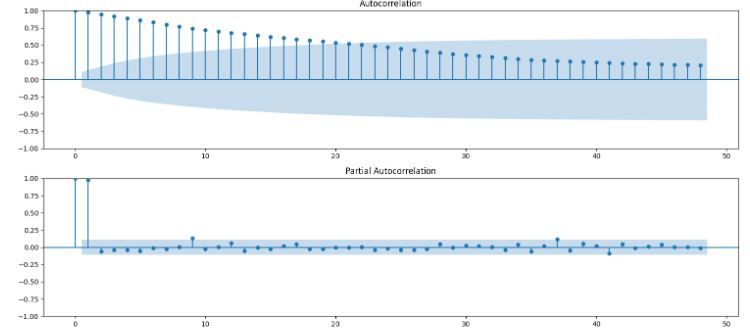
- Training and testing the LSTM Sequential model
df_train = working_data[:-62]
df_test = working_data[-62:]
len(df_train)
258
def create_lookback(dataset, look_back=1):
    X, Y = [], []
    for i in range(len(dataset) - look_back):
        a = dataset[i:(i + look_back), 0]
        X.append(a)
        Y.append(dataset[i + look_back, 0])
    return np.array(X), np.array(Y)
#from sklearn.preprocessing import MinMaxScaler
#from sklearn.preprocessing import minmax_scale
#from sklearn.preprocessing import MaxAbsScaler
#from sklearn.preprocessing import StandardScaler
from sklearn.preprocessing import RobustScaler
#from sklearn.preprocessing import Normalizer
#from sklearn.preprocessing import QuantileTransformer
#from sklearn.preprocessing import PowerTransformer

training_set = df_train.values
training_set = np.reshape(training_set, (len(training_set), 1))
test_set = df_test.values
test_set = np.reshape(test_set, (len(test_set), 1))

#scale datasets
scaler = RobustScaler()
training_set = scaler.fit_transform(training_set)
test_set = scaler.transform(test_set)

# create datasets which are suitable for time series forecasting
look_back = 1
X_train, Y_train = create_lookback(training_set, look_back)
X_test, Y_test = create_lookback(test_set, look_back)

 # reshape datasets so that they will be ok for the requirements of the LSTM model in Keras
X_train = np.reshape(X_train, (len(X_train), 1, X_train.shape[1]))
X_test = np.reshape(X_test, (len(X_test), 1, X_test.shape[1]))
# initialize sequential model, add 2 stacked LSTM layers and densely connected output neuron
model = Sequential()
model.add(LSTM(256, return_sequences=True, input_shape=(X_train.shape[1], X_train.shape[2])))
model.add(LSTM(256))
model.add(Dense(1))

# compile and fit the model
#model.compile(loss='mean_squared_error', optimizer='adam')
#model.compile(loss='mean_squared_error', optimizer='Adamax')
#model.compile(loss='mean_squared_error', optimizer='RMSprop')
model.compile(loss='mean_squared_error', optimizer='Nadam')
history = model.fit(X_train, Y_train, epochs=26, batch_size=16, shuffle=False,
                    validation_data=(X_test, Y_test),
                    callbacks = [EarlyStopping(monitor='val_loss', min_delta=5e-5, patience=20, verbose=2)])
model.summary()
Model: "sequential"
_________________________________________________________________
 Layer (type)                Output Shape              Param #
=================================================================
 lstm (LSTM)                 (None, 1, 256)            264192

 lstm_1 (LSTM)               (None, 256)               525312

 dense (Dense)               (None, 1)                 257

=================================================================
Total params: 789,761
Trainable params: 789,761
Non-trainable params: 0
trace1 = go.Scatter(
    x = np.arange(0, len(history.history['loss']), 1),
    y = history.history['loss'],
    mode = 'lines',
    name = 'Train loss',
    line = dict(color=('rgb(66, 244, 155)'), width=2, dash='dash')
)
trace2 = go.Scatter(
    x = np.arange(0, len(history.history['val_loss']), 1),
    y = history.history['val_loss'],
    mode = 'lines',
    name = 'Test loss',
    line = dict(color=('rgb(244, 146, 65)'), width=2)
)

data = [trace1, trace2]
layout = dict(title = 'Train and Test Loss during training',
              xaxis = dict(title = 'Epoch number'), yaxis = dict(title = 'Loss'))
fig = dict(data=data, layout=layout)
py.iplot(fig, filename='training_process')
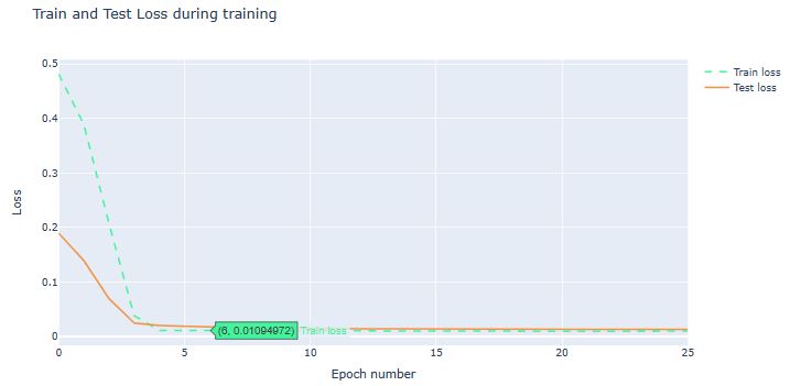
# add one additional data point to align shapes of the predictions and true labels
#X_test = np.append(X_test, scaler.transform(working_data.iloc[-1][0]))
#X_test = np.reshape(X_test, (len(X_test), 1, 1))

# get predictions and then make some transformations to be able to calculate RMSE properly in USD
prediction = model.predict(X_test)
prediction_inverse = scaler.inverse_transform(prediction.reshape(-1, 1))
Y_test_inverse = scaler.inverse_transform(Y_test.reshape(-1, 1))
prediction2_inverse = np.array(prediction_inverse[:,0][1:])
Y_test2_inverse = np.array(Y_test_inverse[:,0])
trace1 = go.Scatter(
    x = np.arange(0, len(prediction2_inverse), 1),
    y = prediction2_inverse,
    mode = 'lines',
    name = 'Predicted price',
    hoverlabel= dict(namelength=-1),
    line = dict(color=('rgb(244, 146, 65)'), width=2)
)
trace2 = go.Scatter(
    x = np.arange(0, len(Y_test2_inverse), 1),
    y = Y_test2_inverse,
    mode = 'lines',
    name = 'True price',
    line = dict(color=('rgb(66, 244, 155)'), width=2)
)

data = [trace1, trace2]
layout = dict(title = 'Comparison of true prices (on the test dataset) with prices our model predicted',
             xaxis = dict(title = 'Day number'), yaxis = dict(title = 'Price, USD'))
fig = dict(data=data, layout=layout)
py.iplot(fig, filename='results_demonstrating0')
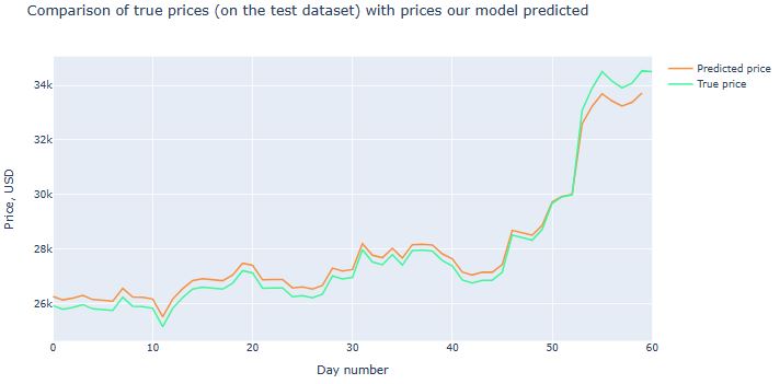
- Let’s look at the BTC-USD time series data within the interval 2020-01-1 and 2023-11-2
import os
os.chdir('YOURPATH')    # Set working directory
os. getcwd()
import datetime
import pandas_datareader.data as web
import datetime
import pandas as pd
pd.set_option('display.max_columns', None)
pd.set_option('display.max_rows', None)
from pandas_datareader import data as pdr
import yfinance as yfin

yfin.pdr_override()

start_date = "2020-01-1"
end_date = "2023-11-2"

btc = pdr.get_data_yahoo("BTC-USD", start_date, end_date)['Close']

print(btc.tail())
[*********************100%***********************]  1 of 1 completed
Date
2023-10-28    34089.574219
2023-10-29    34538.480469
2023-10-30    34502.363281
2023-10-31    34667.781250
2023-11-01    34258.570312
Name: Close, dtype: float64
btc.to_csv("btc.csv")
btc = pd.read_csv("btc.csv")
btc.index = pd.to_datetime(btc['Date'], format='%Y-%m-%d')
del btc['Date']
import matplotlib.pyplot as plt
import seaborn as sns
sns.set()
plt.figure(figsize=(10,6))
plt.plot(btc.index, btc['Close'],linewidth=3)
plt.ylabel('BTC-USD Price')
plt.xlabel('Date')
plt.xticks(rotation=45)
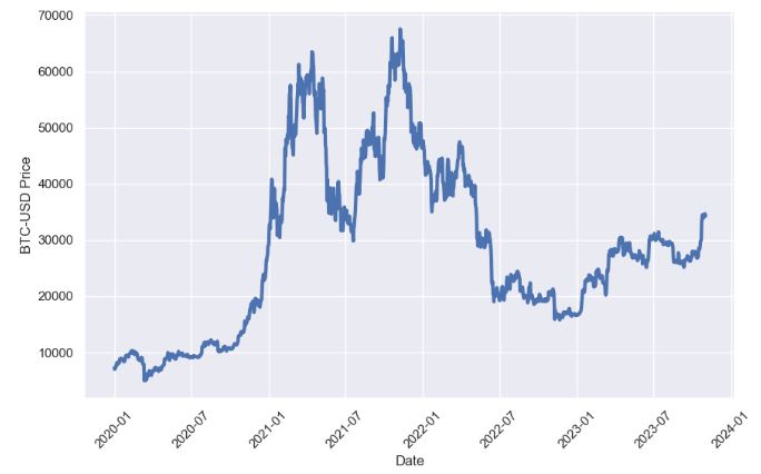
- Train/test splitting the above data with test_date = “2023-07-15”
test_date = "2023-07-15"
train = btc[btc.index < pd.to_datetime(test_date, format='%Y-%m-%d')]
test = btc[btc.index > pd.to_datetime(test_date, format='%Y-%m-%d')]
plt.figure(figsize=(10,6))
plt.plot(train, color = "black",linewidth=3)
plt.plot(test, color = "red",linewidth=3)
plt.ylabel('BTC-USD Price')
plt.xlabel('Date')
plt.xticks(rotation=45)
plt.title("Train/Test split for BTC-USD Data")
plt.show()
- SARIMAX forecast
from statsmodels.tsa.statespace.sarimax import SARIMAX
y = train['Close']
ARMAmodel = SARIMAX(y, order = (1, 0, 1))
# Construct the model
ARMAmodelmod = SARIMAX(y, order=(1, 0, 0), trend='c')
# Estimate the parameters
res = ARMAmodel.fit()

print(res.summary())
                          SARIMAX Results
==============================================================================
Dep. Variable:                  Close   No. Observations:                 1291
Model:               SARIMAX(1, 0, 1)   Log Likelihood              -10981.559
Date:                Wed, 01 Nov 2023   AIC                          21969.118
Time:                        16:15:41   BIC                          21984.607
Sample:                    01-01-2020   HQIC                         21974.931
                         - 07-14-2023
Covariance Type:                  opg
==============================================================================
                 coef    std err          z      P>|z|      [0.025      0.975]
------------------------------------------------------------------------------
ar.L1          0.9997      0.000   2082.623      0.000       0.999       1.001
ma.L1         -0.0305      0.022     -1.410      0.159      -0.073       0.012
sigma2      1.428e+06   2.68e-10   5.32e+15      0.000    1.43e+06    1.43e+06
===================================================================================
Ljung-Box (L1) (Q):                   0.00   Jarque-Bera (JB):              2029.60
Prob(Q):                              0.99   Prob(JB):                         0.00
Heteroskedasticity (H):               0.57   Skew:                            -0.19
Prob(H) (two-sided):                  0.00   Kurtosis:                         9.13
===================================================================================
# The default is to get a one-step-ahead forecast:
print(res.forecast())

2023-07-15    30357.985191
Freq: D, dtype: float64
True value: 30295.81
Difference: 62 or 0.2%

print(res.forecast(steps=2))

2023-07-15    30357.985191
2023-07-16    30348.430872     True value: 30249.13	Difference: 99 or 0.3%
Freq: D, Name: predicted_mean, dtype: float64

fcast_res2 = res.get_forecast(steps=2)
# Note: since we did not specify the alpha parameter, the
# confidence level is at the default, 95%
print(fcast_res2.summary_frame())

Close               mean      mean_se  mean_ci_lower  mean_ci_upper
2023-07-15  30357.985191  1195.074397   28015.682414   32700.287968
2023-07-16  30348.430872  1664.295684   27086.471273   33610.390471

# Here we construct a more complete results object.
fcast_res1 = res.get_forecast()

# Most results are collected in the `summary_frame` attribute.
# Here we specify that we want a confidence level of 90%
print(fcast_res1.summary_frame(alpha=0.10))

Close               mean      mean_se  mean_ci_lower  mean_ci_upper
2023-07-15  30357.985191  1195.074397   28392.262734   32323.707647

print(res.forecast(end_date))

2023-11-02    29324.834244
Freq: D, Name: predicted_mean, dtype: float64
True value: 35388.54  Difference: 6063 or 17%
#y_pred = res.get_forecast(len(train.index))

#Autoregressive Moving Average (ARMA)
y_pred_df = y_pred.conf_int(alpha = 0.05)
y_pred_df["Predictions"] = res.predict(start = y_pred_df.index[0], end = y_pred_df.index[-1])
y_pred_df.index = train.index
y_pred_out = y_pred_df["Predictions"]

y_pred = res.get_forecast(len(test.index))

y_pred_df = y_pred.conf_int(alpha = 0.05)
y_pred_df["Predictions"] = res.predict(start = y_pred_df.index[0], end = y_pred_df.index[-1])
y_pred_df.index = test.index
y_pred_out = y_pred_df["Predictions"]

plt.figure(figsize=(10,6))
plt.plot(train, color = "black",linewidth=3,label = 'Train')
plt.plot(test, color = "red",linewidth=3,label = 'Test')
plt.ylabel('BTC-USD Price')
plt.xlabel('Date')
plt.xticks(rotation=45)
plt.title("Train/Test split for BTC-USD Data")

plt.plot(y_pred_out, color='green', label = 'Predictions')
plt.legend()
plt.show()

import numpy as np
from sklearn.metrics import mean_squared_error

arma_rmse = np.sqrt(mean_squared_error(test["Close"].values, y_pred_df["Predictions"]))
print("RMSE: ",arma_rmse)
RMSE:  3974.586373353312
- SARIMA prediction
#Seasonal ARIMA (SARIMA)
SARIMAXmodel = SARIMAX(y, order = (1, 0, 1), seasonal_order=(2,2,2,2))
SARIMAXmodel = SARIMAXmodel.fit()

y_pred = SARIMAXmodel.get_forecast(len(test.index))
y_pred_df = y_pred.conf_int(alpha = 0.05)
y_pred_df["Predictions"] = SARIMAXmodel.predict(start = y_pred_df.index[0], end = y_pred_df.index[-1])
y_pred_df.index = test.index
y_pred_out = y_pred_df["Predictions"]


plt.figure(figsize=(10,6))
plt.plot(train, color = "black",linewidth=3,label = 'Train')
plt.plot(test, color = "red",linewidth=3,label = 'Test')
plt.ylabel('BTC-USD Price')
plt.xlabel('Date')
plt.xticks(rotation=45)
plt.title("Train/Test split for BTC-USD Data")


plt.plot(y_pred_out, color='Blue', label = 'SARIMA Predictions')
plt.legend()

- Test for stationarity
import os
import warnings
warnings.filterwarnings('ignore')
import numpy as np
import pandas as pd
import matplotlib.pyplot as plt
plt.style.use('fivethirtyeight')
from pylab import rcParams
rcParams['figure.figsize'] = 10, 6
from statsmodels.tsa.stattools import adfuller
from statsmodels.tsa.seasonal import seasonal_decompose
from statsmodels.tsa.arima_model import ARIMA
from pmdarima.arima import auto_arima
from sklearn.metrics import mean_squared_error, mean_absolute_error
import math
import numpy as np

def test_stationarity(timeseries):
    #Determing rolling statistics
    rolmean = timeseries.rolling(12).mean()
    rolstd = timeseries.rolling(12).std()
    #Plot rolling statistics:
    plt.plot(timeseries, color='blue',label='Original')
    plt.plot(rolmean, color='red', label='Rolling Mean')
    plt.plot(rolstd, color='black', label = 'Rolling Std')
    plt.legend(loc='best')
    plt.title('Rolling Mean and Standard Deviation')
    plt.show(block=False)

    print("Results of dickey fuller test")
    adft = adfuller(timeseries,autolag='AIC')
    # output for dft will give us without defining what the values are.
    #hence we manually write what values does it explains using a for loop
    output = pd.Series(adft[0:4],index=['Test Statistics','p-value','No. of lags used','Number of observations used'])
    for key,values in adft[4].items():
        output['critical value (%s)'%key] =  values
    print(output)

test_stationarity(btc)

Results of dickey fuller test
Test Statistics                  -1.795708
p-value                           0.382595
No. of lags used                 24.000000
Number of observations used    1376.000000
critical value (1%)              -3.435111
critical value (5%)              -2.863643
critical value (10%)             -2.567890
dtype: float64
from pylab import rcParams
rcParams['figure.figsize'] = 10, 6
df_log = np.log(btc)
moving_avg = df_log.rolling(12).mean()
std_dev = df_log.rolling(12).std()
plt.legend(loc='best')
plt.title('Moving Average')
plt.plot(std_dev, color ="black", label = "Standard Deviation")
plt.plot(moving_avg, color="red", label = "Mean")
plt.legend()
plt.show()
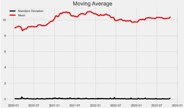
- AutoARIMA training model
#split data into train and training set
train_data, test_data = df_log[3:int(len(df_log)*0.9)], df_log[int(len(df_log)*0.9):]
plt.figure(figsize=(10,6))
plt.grid(True)
plt.xlabel('Dates')
plt.ylabel('Closing Prices')
plt.plot(df_log, 'green', label='Train data')
plt.plot(test_data, 'blue', label='Test data')
plt.legend()

model_autoARIMA = auto_arima(train_data, start_p=0, start_q=0,
                      test='adf',       # use adftest to find             optimal 'd'
                      max_p=3, max_q=3, # maximum p and q
                      m=1,              # frequency of series
                      d=None,           # let model determine 'd'
                      seasonal=False,   # No Seasonality
                      start_P=0,
                      D=0,
                      trace=True,
                      error_action='ignore',
                      suppress_warnings=True,
                      stepwise=True)
print(model_autoARIMA.summary())
 ARIMA(0,1,0)(0,0,0)[0] intercept   : AIC=-4690.298, Time=0.10 sec
 ARIMA(1,1,0)(0,0,0)[0] intercept   : AIC=-4692.481, Time=0.10 sec
 ARIMA(0,1,1)(0,0,0)[0] intercept   : AIC=-4692.115, Time=0.20 sec
 ARIMA(0,1,0)(0,0,0)[0]             : AIC=-4691.403, Time=0.06 sec
 ARIMA(2,1,0)(0,0,0)[0] intercept   : AIC=-4693.266, Time=0.09 sec
 ARIMA(3,1,0)(0,0,0)[0] intercept   : AIC=-4691.517, Time=0.19 sec
 ARIMA(2,1,1)(0,0,0)[0] intercept   : AIC=-4692.222, Time=0.14 sec
 ARIMA(1,1,1)(0,0,0)[0] intercept   : AIC=-4695.721, Time=0.47 sec
 ARIMA(1,1,2)(0,0,0)[0] intercept   : AIC=-4691.365, Time=0.23 sec
 ARIMA(0,1,2)(0,0,0)[0] intercept   : AIC=-4692.743, Time=0.31 sec
 ARIMA(2,1,2)(0,0,0)[0] intercept   : AIC=-4692.995, Time=0.54 sec
 ARIMA(1,1,1)(0,0,0)[0]             : AIC=-4696.473, Time=0.10 sec
 ARIMA(0,1,1)(0,0,0)[0]             : AIC=-4693.116, Time=0.11 sec
 ARIMA(1,1,0)(0,0,0)[0]             : AIC=-4693.478, Time=0.07 sec
 ARIMA(2,1,1)(0,0,0)[0]             : AIC=-4694.922, Time=0.31 sec
 ARIMA(1,1,2)(0,0,0)[0]             : AIC=-4692.402, Time=0.10 sec
 ARIMA(0,1,2)(0,0,0)[0]             : AIC=-4693.807, Time=0.06 sec
 ARIMA(2,1,0)(0,0,0)[0]             : AIC=-4694.351, Time=0.13 sec
 ARIMA(2,1,2)(0,0,0)[0]             : AIC=-4694.577, Time=0.27 sec

Best model:  ARIMA(1,1,1)(0,0,0)[0]
Total fit time: 3.592 seconds
                               SARIMAX Results
==============================================================================
Dep. Variable:                      y   No. Observations:                 1257
Model:               SARIMAX(1, 1, 1)   Log Likelihood                2351.236
Date:                Wed, 01 Nov 2023   AIC                          -4696.473
Time:                        16:23:29   BIC                          -4681.066
Sample:                    01-04-2020   HQIC                         -4690.682
                         - 06-13-2023
Covariance Type:                  opg
==============================================================================
                 coef    std err          z      P>|z|      [0.025      0.975]
------------------------------------------------------------------------------
ar.L1         -0.6677      0.163     -4.086      0.000      -0.988      -0.347
ma.L1          0.6052      0.174      3.469      0.001       0.263       0.947
sigma2         0.0014   1.68e-05     82.299      0.000       0.001       0.001
===================================================================================
Ljung-Box (L1) (Q):                   0.13   Jarque-Bera (JB):             24042.27
Prob(Q):                              0.71   Prob(JB):                         0.00
Heteroskedasticity (H):               0.54   Skew:                            -1.63
Prob(H) (two-sided):                  0.00   Kurtosis:                        24.18
===================================================================================
model_autoARIMA.plot_diagnostics(figsize=(15,8))
plt.show()
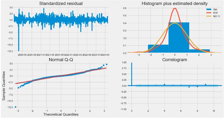
# density plot of residuals
residuals.plot(kind='kde')
plt.show()

# summary stats of residuals
print(residuals.describe())
                0
count  1257.000000
mean      0.007939
std       0.254041
min      -0.461884
25%      -0.014908
50%       0.000702
75%       0.017431
max       8.910674
- Let’s look at the BTC-USD price in 2023
from pandas_datareader import data as pdr
import yfinance as yfin

yfin.pdr_override()

start_date = "2023-01-1"
end_date = "2023-11-1"

stock_data = pdr.get_data_yahoo("BTC-USD", start_date, end_date)

print(stock_data.head())

[*********************100%***********************]  1 of 1 completed
                    Open          High           Low         Close  \
Date
2023-01-01  16547.914062  16630.439453  16521.234375  16625.080078
2023-01-02  16625.509766  16759.343750  16572.228516  16688.470703
2023-01-03  16688.847656  16760.447266  16622.371094  16679.857422
2023-01-04  16680.205078  16964.585938  16667.763672  16863.238281
2023-01-05  16863.472656  16884.021484  16790.283203  16836.736328

               Adj Close       Volume
Date
2023-01-01  16625.080078   9244361700
2023-01-02  16688.470703  12097775227
2023-01-03  16679.857422  13903079207
2023-01-04  16863.238281  18421743322
2023-01-05  16836.736328  13692758566

#plot close price
plt.figure(figsize=(10,6))
plt.grid(True)
plt.xlabel('Date')
plt.ylabel('Close Prices')
plt.plot(stock_data['Close'])
plt.title('BTC-USD closing price')
plt.show(
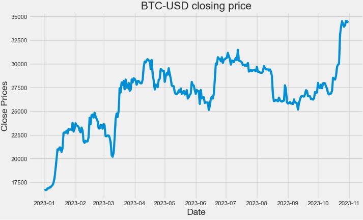
df_close=stock_data['Close']
#Distribution of the dataset
df_close.plot(kind='kde')

- Test of stationarity
#Test for staionarity
def test_stationarity(timeseries):
    #Determing rolling statistics
    rolmean = timeseries.rolling(12).mean()
    rolstd = timeseries.rolling(12).std()
    #Plot rolling statistics:
    plt.plot(timeseries, color='blue',label='Original')
    plt.plot(rolmean, color='red', label='Rolling Mean')
    plt.plot(rolstd, color='black', label = 'Rolling Std')
    plt.legend(loc='best')
    plt.title('Rolling Mean and Standard Deviation')
    plt.show(block=False)

    print("Results of dickey fuller test")
    adft = adfuller(timeseries,autolag='AIC')
    # output for dft will give us without defining what the values are.
    #hence we manually write what values does it explains using a for loop
    output = pd.Series(adft[0:4],index=['Test Statistics','p-value','No. of lags used','Number of observations used'])
    for key,values in adft[4].items():
        output['critical value (%s)'%key] =  values
    print(output)

test_stationarity(df_close)

Results of dickey fuller test
Test Statistics                 -2.147033
p-value                          0.226028
No. of lags used                 0.000000
Number of observations used    303.000000
critical value (1%)             -3.452118
critical value (5%)             -2.871127
critical value (10%)            -2.571878
dtype: float64
#To separate the trend and the seasonality from a time series,
# we can decompose the series using the following code.
result = seasonal_decompose(df_close, model='multiplicative')
fig = plt.figure()
fig = result.plot()
fig.set_size_inches(16, 9)

#if not stationary then eliminate trend
#Eliminate trend
from pylab import rcParams
rcParams['figure.figsize'] = 10, 6
df_log = np.log(df_close)
moving_avg = df_log.rolling(12).mean()
std_dev = df_log.rolling(12).std()
plt.legend(loc='best')
plt.title('Moving Average')
plt.plot(std_dev, color ="black", label = "Standard Deviation")
plt.plot(moving_avg, color="red", label = "Mean")
plt.legend()
plt.show()
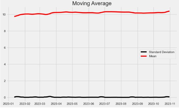
- Train/test data splitting
#split data into train and training set
train_data, test_data = df_log[3:int(len(df_log)*0.9)], df_log[int(len(df_log)*0.9):]
plt.figure(figsize=(10,6))
plt.grid(True)
plt.xlabel('Dates')
plt.ylabel('Closing Prices')
plt.plot(df_log, 'green', label='Train data')
plt.plot(test_data, 'blue', label='Test data')
plt.legend()
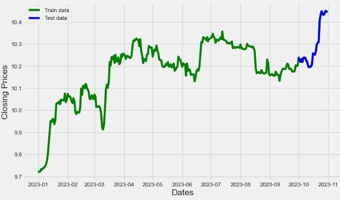
model_autoARIMA = auto_arima(train_data, start_p=0, start_q=0,
                      test='adf',       # use adftest to find optimal 'd'
                      max_p=3, max_q=3, # maximum p and q
                      m=1,              # frequency of series
                      d=None,           # let model determine 'd'
                      seasonal=False,   # No Seasonality
                      start_P=0,
                      D=0,
                      trace=True,
                      error_action='ignore',
                      suppress_warnings=True,
                      stepwise=True)
print(model_autoARIMA.summary())
model_autoARIMA.plot_diagnostics(figsize=(15,8))
plt.show()
Performing stepwise search to minimize aic
 ARIMA(0,0,0)(0,0,0)[0]             : AIC=2021.064, Time=0.01 sec
 ARIMA(1,0,0)(0,0,0)[0]             : AIC=inf, Time=0.07 sec
 ARIMA(0,0,1)(0,0,0)[0]             : AIC=inf, Time=0.05 sec
 ARIMA(1,0,1)(0,0,0)[0]             : AIC=-1257.660, Time=0.12 sec
 ARIMA(2,0,1)(0,0,0)[0]             : AIC=-1247.088, Time=0.14 sec
 ARIMA(1,0,2)(0,0,0)[0]             : AIC=-1257.580, Time=0.18 sec
 ARIMA(0,0,2)(0,0,0)[0]             : AIC=inf, Time=0.08 sec
 ARIMA(2,0,0)(0,0,0)[0]             : AIC=inf, Time=0.08 sec
 ARIMA(2,0,2)(0,0,0)[0]             : AIC=-1251.411, Time=0.25 sec
 ARIMA(1,0,1)(0,0,0)[0] intercept   : AIC=-1262.180, Time=0.18 sec
 ARIMA(0,0,1)(0,0,0)[0] intercept   : AIC=-637.358, Time=0.07 sec
 ARIMA(1,0,0)(0,0,0)[0] intercept   : AIC=-1264.320, Time=0.14 sec
 ARIMA(0,0,0)(0,0,0)[0] intercept   : AIC=-336.312, Time=0.04 sec
 ARIMA(2,0,0)(0,0,0)[0] intercept   : AIC=-1262.524, Time=0.20 sec
 ARIMA(2,0,1)(0,0,0)[0] intercept   : AIC=-1247.437, Time=0.31 sec

Best model:  ARIMA(1,0,0)(0,0,0)[0] intercept
Total fit time: 1.948 seconds
                               SARIMAX Results
==============================================================================
Dep. Variable:                      y   No. Observations:                  270
Model:               SARIMAX(1, 0, 0)   Log Likelihood                 635.160
Date:                Tue, 31 Oct 2023   AIC                          -1264.320
Time:                        17:24:09   BIC                          -1253.525
Sample:                    01-04-2023   HQIC                         -1259.985
                         - 09-30-2023
Covariance Type:                  opg
==============================================================================
                 coef    std err          z      P>|z|      [0.025      0.975]
------------------------------------------------------------------------------
intercept      0.1320      0.067      1.979      0.048       0.001       0.263
ar.L1          0.9869      0.007    147.729      0.000       0.974       1.000
sigma2         0.0005    2.8e-05     18.439      0.000       0.000       0.001
===================================================================================
Ljung-Box (L1) (Q):                   0.49   Jarque-Bera (JB):               101.66
Prob(Q):                              0.48   Prob(JB):                         0.00
Heteroskedasticity (H):               0.30   Skew:                             0.56
Prob(H) (two-sided):                  0.00   Kurtosis:                         5.79
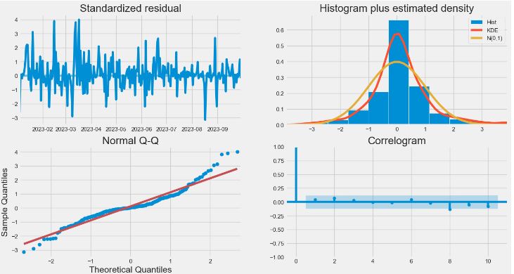
# Forecast
fc, se, conf = fitted.forecast(3, alpha=0.05)  # 95% conf
print (fc)
10.202972895932403
from pandas import read_csv
from pandas import datetime
from matplotlib import pyplot
from statsmodels.tsa.arima.model import ARIMA
from sklearn.metrics import mean_squared_error
from math import sqrt
# load dataset


train, test = train_data, test_data
history = [x for x in train]
predictions = list()
# walk-forward validation
for t in range(len(test)):
 model = ARIMA(history, order=(1,1,2))
 model_fit = model.fit()
 output = model_fit.forecast()
 yhat = output[0]
 predictions.append(yhat)
 obs = test[t]
 history.append(obs)
 print('predicted=%f, expected=%f' % (yhat, obs))
# evaluate forecasts
rmse = sqrt(mean_squared_error(test, predictions))
print('Test RMSE: %.3f' % rmse)

predicted=10.317140, expected=10.331632
predicted=10.331451, expected=10.311823
predicted=10.311999, expected=10.323689
predicted=10.322517, expected=10.324736
predicted=10.325448, expected=10.328431
predicted=10.329127, expected=10.329434
predicted=10.330061, expected=10.346776
predicted=10.347997, expected=10.334542
predicted=10.336030, expected=10.325946
predicted=10.324786, expected=10.305926
predicted=10.303358, expected=10.320297
predicted=10.318232, expected=10.318657
predicted=10.319422, expected=10.314644
predicted=10.314766, expected=10.322674
predicted=10.322678, expected=10.329440
predicted=10.330562, expected=10.321923
predicted=10.322634, expected=10.356982
predicted=10.358162, expected=10.320027
predicted=10.322579, expected=10.318765
predicted=10.315681, expected=10.317223
Test RMSE: 0.016

print(test_data.index)
DatetimeIndex(['2023-06-27', '2023-06-28', '2023-06-29', '2023-06-30',
               '2023-07-01', '2023-07-02', '2023-07-03', '2023-07-04',
               '2023-07-05', '2023-07-06', '2023-07-07', '2023-07-08',
               '2023-07-09', '2023-07-10', '2023-07-11', '2023-07-12',
               '2023-07-13', '2023-07-14', '2023-07-15', '2023-07-16'],
              dtype='datetime64[ns]', name='Date', freq=None)
- Let’s apply the 60-day LSTM forecasting algorithm to BTC-USD 2023 price
import numpy as np
import pandas as pd
import matplotlib.pyplot as plt
from keras.models import Sequential
from keras.layers import Dense, LSTM
import math
from sklearn.preprocessing import MinMaxScaler,StandardScaler,RobustScaler
import pandas_datareader.data as web
import datetime
import pandas as pd
pd.set_option('display.max_columns', None)
pd.set_option('display.max_rows', None)
#Reading and Displaying BTC Time Series Data

from pandas_datareader import data as pdr
import yfinance as yfin

yfin.pdr_override()

start_date = "2023-01-1"
end_date = "2023-11-2"

btc = pdr.get_data_yahoo("BTC-USD", start_date, end_date)

#print(btc.head())
#  Plotting date vs the close market stock price
final_data=btc
final_data['Date'] = btc.index
#final_data.plot('Date','Close',color="red")
# Extract only top 60 rows to make the plot a little clearer
new_data = final_data.head(60)

#  Plotting date vs the close  market stock price
#new_data.plot('Date','Close',color="green")

#plt.show()

#Creating a new Dataframe and Training data
# 1. Filter out the closing market price data
close_data = final_data.filter(['Close'])

# 2. Convert the data into array for easy evaluation
dataset = close_data.values
datasetindex=close_data.index

# 3. Scale/Normalize the data to make all values between 0 and 1
scaler = RobustScaler()
scaled_data = scaler.fit_transform(dataset)

# 4. Creating training data size : 80% of the data
training_data_len = math.ceil(len(dataset) *.8)
train_data = scaled_data[0:training_data_len  , : ]

# 5. Separating the data into x and y data
x_train_data=[]
y_train_data =[]
for i in range(30,len(train_data)):
    x_train_data=list(x_train_data)
    y_train_data=list(y_train_data)
    x_train_data.append(train_data[i-30:i,0])
    y_train_data.append(train_data[i,0])

    # 6. Converting the training x and y values to numpy arrays
    x_train_data1, y_train_data1 = np.array(x_train_data), np.array(y_train_data)

    # 7. Reshaping training s and y data to make the calculations easier
    x_train_data2 = np.reshape(x_train_data1, (x_train_data1.shape[0],x_train_data1.shape[1],1))
#Building LSTM Model
model = Sequential()
model.add(LSTM(units=50, return_sequences=True,input_shape=(x_train_data2.shape[1],1)))
model.add(LSTM(units=50, return_sequences=False))
model.add(Dense(units=25))
model.add(Dense(units=1))
model.summary()
Model: "sequential_1"
_________________________________________________________________
 Layer (type)                Output Shape              Param #
=================================================================
 lstm_2 (LSTM)               (None, 30, 50)            10400

 lstm_3 (LSTM)               (None, 50)                20200

 dense_2 (Dense)             (None, 25)                1275

 dense_3 (Dense)             (None, 1)                 26

=================================================================
Total params: 31,901
Trainable params: 31,901
Non-trainable params: 0
model.compile(optimizer='adam', loss='mean_squared_error')
history=model.fit(x_train_data2, y_train_data1, batch_size=1, epochs=3)

Epoch 1/3
214/214 [==============================] - 3s 8ms/step - loss: 0.1226
Epoch 2/3
214/214 [==============================] - 2s 8ms/step - loss: 0.0622
Epoch 3/3
214/214 [==============================] - 2s 7ms/step - loss: 0.0492
plt.plot(history.history['loss'], label='train')
plt.legend()
plt.xlabel('Epoch')
plt.ylabel('MSE Loss')
plt.title('LSTM BTC-USD Test Prediction Q1 2023')
plt.show()
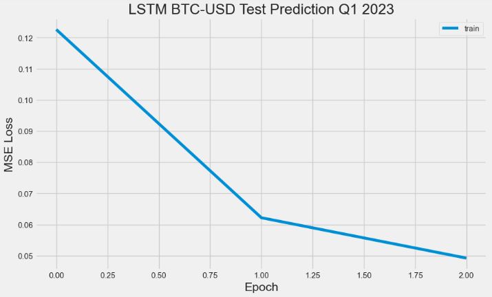
#Testing the model on testing data
# 1. Creating a dataset for testing
test_data = scaled_data[training_data_len - 30: , : ]
test_index=datasetindex[training_data_len - 30:]
x_test = []
y_test =  dataset[training_data_len : , : ]
for i in range(30,len(test_data)):
    x_test.append(test_data[i-30:i,0])

# 2.  Convert the values into arrays for easier computation
x_test = np.array(x_test)
x_test = np.reshape(x_test, (x_test.shape[0],x_test.shape[1],1))

# 3. Making predictions on the testing data
predictions = model.predict(x_test)
predictions = scaler.inverse_transform(predictions)
#Error Calculation
rmse=np.sqrt(np.mean(((predictions- y_test)**2)))
print(rmse)
#Make Predictions
train = scaled_data[:training_data_len]
valid = scaled_data[training_data_len:]

valid['Predictions'] = predictions

plt.plot(predictions,label='predictions')
plt.plot(y_test,label='test data')
plt.legend(loc="upper left")
plt.title("BTC-USD Test Data vs LSTM Predictions")
plt.xlabel("Forecast Day")
plt.ylabel("Price USD")

Natural Gas Price Forecasting
- Reading input NGUSD data from FMP API
import os
os.chdir('YOURPATH') # Set working directory
os. getcwd()
import numpy as np
np.random.seed(3363)
import pandas as pd
from scipy.stats import norm
import datetime
import matplotlib.pyplot as plt
%matplotlib inline
ticker = "NGUSD" #US natural gas
base = 'https://financialmodelingprep.com/api/v3/'
key = 'YOUR API KEY'
target = "{}historical-price-full/{}?apikey={}".format(base, ticker, key)
df = pd.read_json(target)
df = pd.json_normalize(df['historical'])
df['date'] = pd.to_datetime(df['date'])
df.set_index('date', inplace=True)
# saving the file
df.to_csv('NGUSD data.csv')
df.head()
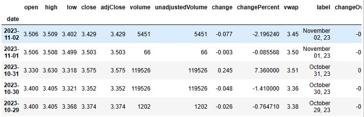
#Plot of asset historical closing price
import matplotlib.pyplot as plt
plt.rcParams.update({'font.size': 16})
df['adjClose'].plot(figsize=(14, 6), title = "Price of {} from {} to {}".format(ticker, df.index.min(), df.index.max()))
plt.grid()

- Stochastic Monte Carlo simulation
#Geometric Brownian Motion
pred_end_date = datetime.datetime(2023, 10, 27)
forecast_dates = [d if d.isoweekday() in range(1, 6) else np.nan for d in pd.date_range(df.index.max(), pred_end_date)]
intervals = len(forecast_dates)
iterations = 1000
#Preparing log returns from data
log_returns = np.log(1 + df['adjClose'].pct_change())
#Setting up drift and random component in relation to asset data
u = log_returns.mean()
var = log_returns.var()
drift = u - (0.5 * var)
stdev = log_returns.std()
daily_returns = np.exp(drift + stdev * norm.ppf(np.random.rand(intervals, iterations)))
del df['Date']
df.head()
Price
Date
1997-01-07 3.82
1997-01-08 3.80
1997-01-09 3.61
1997-01-10 3.92
1997-01-11 3.92
df.tail()
Price
Date
2020-08-28 2.46
2020-08-29 2.46
2020-08-30 2.46
2020-08-31 2.30
2020-09-01 2.22
#Takes last data point as startpoint point for simulation
S0 = df['Price'].iloc[-1]
price_list = np.zeros_like(daily_returns)
price_list[0] = S0
print (S0)
2.22
#Applies Monte Carlo simulation in asset
for t in range(1, intervals):
price_list[t] = price_list[t - 1] * daily_returns[t]
#Plot
import seaborn as sns
sns.distplot(log_returns.iloc[1:])
sns.set(font_scale=2)
plt.xlabel("Daily Return")
plt.ylabel("Frequency")
plt.grid()

u = log_returns.mean()
var = log_returns.var()
drift = u - (0.5*var)
stdev = log_returns.std()
days = 50
trials = 1000
Z = norm.ppf(np.random.rand(days, trials)) #days, trials
daily_returns = np.exp(drift + stdev * Z)
from IPython.core.display import display, HTML
display(HTML("<style>div.output_scroll { height: 144em; }</style>"))
price_paths = np.zeros_like(daily_returns)
price_paths[0] = S0
for t in range(1, days):
price_paths[t] = price_paths[t-1]*daily_returns[t]
plt.plot(price_paths)
plt.xlabel('Time (days)')
plt.ylabel('NGUSD Price')

- Let’s fit the ARIMA model
from sklearn.metrics import mean_squared_error
from math import sqrt
from statsmodels.tsa.arima.model import ARIMA
# fit ARIMA model
model = ARIMA(df['adjClose'], order=(5,1,0))
model_fit = model.fit()
# summary of fit model
print(model_fit.summary())
# line plot of residuals
residuals = pd.DataFrame(model_fit.resid)
residuals.plot()
plt.show()
# density plot of residuals
residuals.plot(kind='kde')
plt.show()
# summary stats of residuals
print(residuals.describe())
SARIMAX Results
==============================================================================
Dep. Variable: adjClose No. Observations: 1320
Model: ARIMA(5, 1, 0) Log Likelihood 244.542
Date: Thu, 02 Nov 2023 AIC -477.084
Time: 14:52:59 BIC -445.976
Sample: 0 HQIC -465.421
- 1320
Covariance Type: opg
==============================================================================
coef std err z P>|z| [0.025 0.975]
------------------------------------------------------------------------------
ar.L1 -0.1152 0.013 -8.718 0.000 -0.141 -0.089
ar.L2 -0.0343 0.019 -1.820 0.069 -0.071 0.003
ar.L3 0.0113 0.016 0.688 0.492 -0.021 0.043
ar.L4 0.0759 0.018 4.328 0.000 0.042 0.110
ar.L5 -0.0662 0.017 -3.933 0.000 -0.099 -0.033
sigma2 0.0404 0.001 57.115 0.000 0.039 0.042
===================================================================================
Ljung-Box (L1) (Q): 0.03 Jarque-Bera (JB): 7304.45
Prob(Q): 0.87 Prob(JB): 0.00
Heteroskedasticity (H): 0.15 Skew: 0.46
Prob(H) (two-sided): 0.00 Kurtosis: 14.49
===================================================================================
NG residual and density plot of residuals:

0
count 1320.000000
mean 0.002717
std 0.222071
min -1.712644
25% -0.066907
50% -0.001321
75% 0.063192
max 3.429000
Plot ARIMA forecasts against actual outcomes
series = df['adjClose']
series.index = df['adjClose'].index
# split into train and test sets
X = series.values
size = int(len(X) * 0.66)
train, test = X[0:size], X[size:len(X)]
history = [x for x in train]
predictions = list()
# walk-forward validation
for t in range(len(test)):
model = ARIMA(history, order=(5,1,0))
model_fit = model.fit()
output = model_fit.forecast()
yhat = output[0]
predictions.append(yhat)
obs = test[t]
history.append(obs)
#print('predicted=%f, expected=%f' % (yhat, obs))
# evaluate forecasts
rmse = sqrt(mean_squared_error(test, predictions))
print('Test RMSE: %.3f' % rmse)
# plot forecasts against actual outcomes
plt.plot(test)
plt.plot(predictions, color='red')
plt.show()
Test RMSE: 0.103
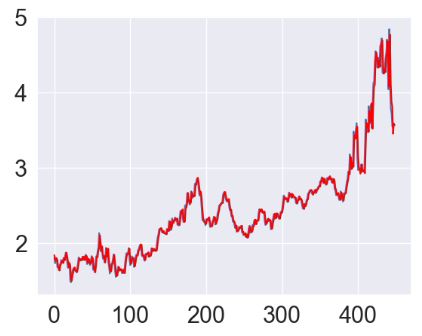
Here red curve means predictions, while blue curve is the actual test NG data.
- Let’s look at the FB Prophet prediction
from prophet import Prophet
# data must be formated for Prophet
[X, Y] = df.index, df['adjClose']
p = pd.DataFrame(Y, X)
p.reset_index(inplace=True)
p.rename(columns={'date': 'ds', 'adjClose': 'y'}, inplace=True)
m = Prophet()
m.fit(p)
future = m.make_future_dataframe(periods=5)
future.tail()
forecast = m.predict(future)
forecast[['ds', 'yhat', 'yhat_lower', 'yhat_upper']].tail()
fig1 = m.plot(forecast)

- Let’s implement the Decision Trees algorithm to predict the NGUSD price
#NG data preparation
df1=df.reset_index(drop=False)
df1['year'] = pd.DatetimeIndex(df1['date']).year
df1['month'] = pd.DatetimeIndex(df1['date']).month
df1['day'] = pd.DatetimeIndex(df1['date']).day
df1.drop('date', axis=1, inplace=True)
df1['close'].fillna(df1['close'].mean(),inplace=True)
import seaborn as sns
sns.lineplot(x='year',y='close',data=df1,color='red')

import seaborn as sns
sns.lineplot(x='month',y='close',data=df1,color='red')

import seaborn as sns
sns.lineplot(x='day',y='close',data=df1,color='red')
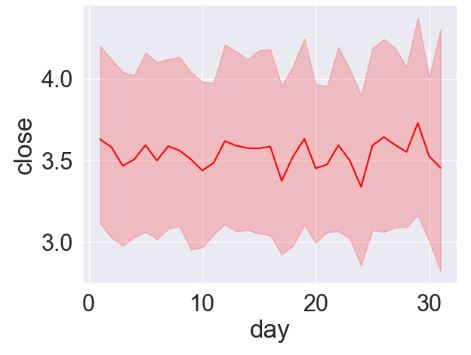
Training and testing the DecisionTreeRegressor with train/test split as 70:30%
x=df1[['year','month','day']].values #inputs
y=df1['close'].values #output price only
from sklearn.model_selection import train_test_split
x_train,x_test,y_train,y_test=train_test_split(x,y,test_size=0.3,random_state=0)
#import decision tree regressor
from sklearn.tree import DecisionTreeRegressor
dtr=DecisionTreeRegressor()
#fitting the model or training the model
dtr.fit(x_train,y_train)
DecisionTreeRegressor:
DecisionTreeRegressor()
y_pred=dtr.predict(x_test)
from sklearn.metrics import r2_score
accuracy=r2_score(y_test,y_pred)
accuracy
0.983484120975274
plt.scatter(y_test,y_pred)
plt.xlabel('Test Data')
plt.ylabel('Predictions')
plt.title('NGUSD Price')
NGUSD price X-plot: test data vs ML predictions:

plt.figure(figsize=(14,6))
plt.plot(y_test,label='Test')
plt.plot(y_pred,label='Predict')
plt.legend(['Test', 'Predict'])
plt.xlabel('Time Index')
plt.ylabel('NGUSD Price')
NGUSD time series: test data vs ML predictions:

- Let’s look at the historical NGUSD data
df = pd.read_csv("NGUSD data.csv")
df0=df[['date','close']]
data = df0.set_index('date')
data.head(3)
close
date
2023-11-02 3.429
2023-11-01 3.503
2023-10-31 3.575
import warnings
import pandas as pd
import numpy as np
import matplotlib.pyplot as plt
warnings.filterwarnings("ignore")
import tensorflow as tf
import os
from tensorflow.keras import layers, models
os.environ['TF_CPP_MIN_LOG_LEVEL'] = '3'
from sklearn.metrics import mean_squared_error, r2_score
import statsmodels.api as sm
import plotly.express as px
from statsmodels.tsa.stattools import adfuller
from statsmodels.graphics.tsaplots import plot_acf, plot_pacf
fig = px.line(data, title = 'Natural Gas Spot Prices', template = 'plotly_dark')
fig.show()

fig = px.histogram(data, x = "close", template = 'plotly_dark')
fig.show()

Test of stationarity while performing the Dickey-Fuller Test:
def test_stationarity(timeseries):
# Determing rolling statistics
rolmean = timeseries.rolling(25).mean()
rolstd = timeseries.rolling(25).std()
# Plot rolling statistics:
plt.figure(figsize = (20,10))
orig = plt.plot(timeseries, color='blue',label='Original')
mean = plt.plot(rolmean, color='red', label='Rolling Mean')
std = plt.plot(rolstd, color='black', label = 'Rolling Std')
plt.legend(loc='best')
plt.title('Rolling Mean & Standard Deviation')
plt.show(block=False)
# Perform Dickey-Fuller test:
print('Results of Dickey-Fuller Test:')
dftest = adfuller(timeseries, autolag = 'AIC')
dfoutput = pd.Series(dftest[0:4], index = ['Test Statistic','p-value','#Lags Used','Number of Observations Used'])
for key,value in dftest[4].items():
dfoutput['Critical Value (%s)'%key] = value
print(dfoutput)
test_stationarity(data)
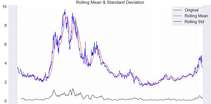
Results of Dickey-Fuller Test:
Test Statistic -2.075628
p-value 0.254427
#Lags Used 16.000000
Number of Observations Used 1303.000000
Critical Value (1%) -3.435379
Critical Value (5%) -2.863761
Critical Value (10%) -2.567952
dtype: float64
EWMA Differences
ts_sqrt = np.sqrt(data)
expwighted_avg = ts_sqrt.ewm(halflife = 25).mean()
ts_sqrt_ewma_diff = ts_sqrt - expwighted_avg
test_stationarity(ts_sqrt_ewma_diff)

Results of Dickey-Fuller Test:
Test Statistic -3.751435
p-value 0.003445
#Lags Used 6.000000
Number of Observations Used 1313.000000
Critical Value (1%) -3.435340
Critical Value (5%) -2.863744
Critical Value (10%) -2.567943
dtype: float64
NG SQRT Differences
ts_sqrt_diff = ts_sqrt - ts_sqrt.shift()
ts_sqrt = np.sqrt(data)
ts_sqrt_diff = ts_sqrt - ts_sqrt.shift()
ts_sqrt_diff.dropna(inplace = True)
test_stationarity(ts_sqrt_diff)

Results of Dickey-Fuller Test:
Test Statistic -1.618360e+01
p-value 4.241417e-29
#Lags Used 5.000000e+00
Number of Observations Used 1.313000e+03
Critical Value (1%) -3.435340e+00
Critical Value (5%) -2.863744e+00
Critical Value (10%) -2.567943e+00
dtype: float64
- ARIMA model predictions
data = data.sort_values(by = 'date')
train = data['2018-11-02': '2023-05-26']
test = data['2023-05-27': '2023-10-27']
print("Length of Train Data: ", len(train))
print("Length of Test Data: ", len(test))
Length of Train Data: 1183
Length of Test Data: 132
Plotting ACF
plt.rcParams.update({'figure.figsize':(12,15), 'figure.dpi':120})
# Original Series
fig, axes = plt.subplots(4, 2, sharex=True)
axes[0, 0].plot(data.close); axes[0, 0].set_title('Original Series')
plot_acf(data.close, ax=axes[0, 1])
# 1st Differencing
axes[1, 0].plot(data.close.diff()); axes[1, 0].set_title('1st Order Differencing')
plot_acf(data.close.diff().dropna(), ax=axes[1, 1])
# 2nd Differencing
axes[2, 0].plot(data.close.diff().diff()); axes[2, 0].set_title('2nd Order Differencing')
plot_acf(data.close.diff().diff().dropna(), ax=axes[2, 1])
# 3rd Differencing
axes[3, 0].plot(data.close.diff().diff().diff()); axes[3, 0].set_title('3nd Order Differencing')
plot_acf(data.close.diff().diff().diff().dropna(), ax=axes[3, 1])
plt.show()
Comparing original series, 1st and 2nd order differencing ACF

Comparing ACF 2nd order vs 3rd order differencing
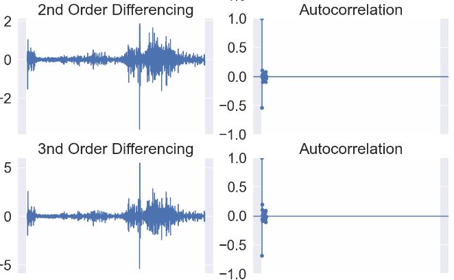
Focus on 1st Differencing and PACF
plt.rcParams.update({'figure.figsize':(12,6), 'figure.dpi':120})
fig, axes = plt.subplots(1, 2, sharex=True)
axes[0].plot(data.close.diff()); axes[0].set_title('1st Differencing')
axes[1].set(ylim=(0,5))
plot_pacf(data.close.diff().dropna(), ax=axes[1])
plt.show()
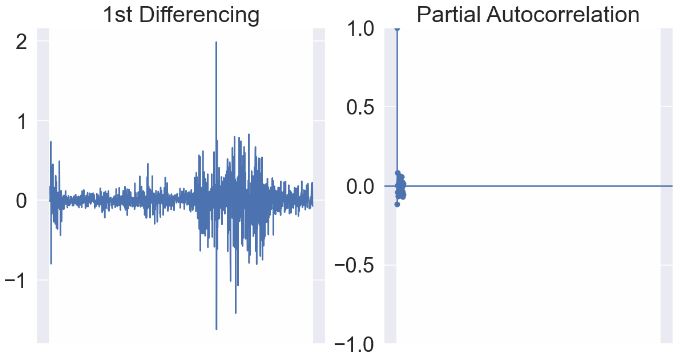
model = sm.tsa.arima.ARIMA(train, order = (1, 2, 1))
arima_model = model.fit()
print(arima_model.summary())
SARIMAX Results
==============================================================================
Dep. Variable: close No. Observations: 1183
Model: ARIMA(1, 2, 1) Log Likelihood 154.295
Date: Thu, 02 Nov 2023 AIC -302.589
Time: 15:14:26 BIC -287.367
Sample: 0 HQIC -296.851
- 1183
Covariance Type: opg
==============================================================================
coef std err z P>|z| [0.025 0.975]
------------------------------------------------------------------------------
ar.L1 -0.1169 0.012 -9.421 0.000 -0.141 -0.093
ma.L1 -0.9997 0.013 -79.323 0.000 -1.024 -0.975
sigma2 0.0448 0.001 49.607 0.000 0.043 0.047
===================================================================================
Ljung-Box (L1) (Q): 0.03 Jarque-Bera (JB): 8520.40
Prob(Q): 0.85 Prob(JB): 0.00
Heteroskedasticity (H): 9.27 Skew: -0.08
Prob(H) (two-sided): 0.00 Kurtosis: 16.16
===================================================================================
yp_train = arima_model.predict(start = 0, end = (len(train)-1))
yp_test = arima_model.predict(start = 0, end = (len(test)-1))
print("Train Data:\nMean Square Error: {}".format(mean_squared_error(train, yp_train)))
print("\nTest Data:\nMean Square Error: {}".format(mean_squared_error(test, yp_test)))
slot = 15
x_train = []
y_train = []
for i in range(slot, len(train)):
x_train.append(train.iloc[i-slot:i, 0])
y_train.append(train.iloc[i, 0])
x_train, y_train = np.array(x_train), np.array(y_train)
x_train = np.reshape(x_train, (x_train.shape[0], x_train.shape[1], 1))
print(x_train.shape, y_train.shape)
(1168, 15, 1) (1168,)
- LSTM Keras prediction
lstm_model = tf.keras.Sequential()
lstm_model.add(tf.keras.layers.LSTM(units = 50, input_shape = (slot, 1), return_sequences = True, activation = 'relu'))
#lstm_model.add(tf.keras.layers.Dropout(0.01))
lstm_model.add(tf.keras.layers.LSTM(units = 50, activation = 'relu', return_sequences = True))
#lstm_model.add(tf.keras.layers.Dropout(0.01))
lstm_model.add(tf.keras.layers.LSTM(units = 50, return_sequences = True))
#lstm_model.add(tf.keras.layers.Dropout(0.01))
lstm_model.add(tf.keras.layers.LSTM(units = 50, return_sequences = False))
#lstm_model.add(tf.keras.layers.Dropout(0.01))
lstm_model.add(tf.keras.layers.Dense(units = 1))
lstm_model.compile(loss = 'mean_squared_error', optimizer = 'adam')
lstm_model.summary()
Model: "sequential"
_________________________________________________________________
Layer (type) Output Shape Param #
=================================================================
lstm (LSTM) (None, 15, 50) 10400
lstm_1 (LSTM) (None, 15, 50) 20200
lstm_2 (LSTM) (None, 15, 50) 20200
lstm_3 (LSTM) (None, 50) 20200
dense (Dense) (None, 1) 51
=================================================================
Total params: 71,051
Trainable params: 71,051
Non-trainable params: 0
_________________________________________________________________
early_stopping = tf.keras.callbacks.EarlyStopping(monitor = 'loss', patience = 7)
history = lstm_model.fit(x_train, y_train, epochs = 100,
batch_size = 64,
verbose = 1, shuffle = False,
callbacks = [early_stopping])
yp_train = lstm_model.predict(x_train)
a = pd.DataFrame(yp_train)
a.rename(columns = {0: 'gp_pred'}, inplace = True);
a.index = train.iloc[slot:].index
train_compare = pd.concat([train.iloc[slot:], a], 1)
plt.figure(figsize = (15, 5))
plt.plot(train_compare['close'], color = 'red', label = "Actual Natural Gas Price")
plt.plot(train_compare['gp_pred'], color = 'blue', label = 'Predicted Price')
plt.title("Natural Gas Price Prediction on Train Data")
plt.xlabel('Time')
plt.ylabel('Natural gas price')
plt.legend(loc = 'best')
import matplotlib
matplotlib.rcParams.update({'font.size': 12})
plt.show()

data_new = np.roll(train_compare['gp_pred'], -4)
plt.plot(data_new,label='Predict',lw=3)
plt.plot(train_compare['close'],label='Train',lw=3)
matplotlib.rcParams.update({'font.size': 12})
plt.legend()
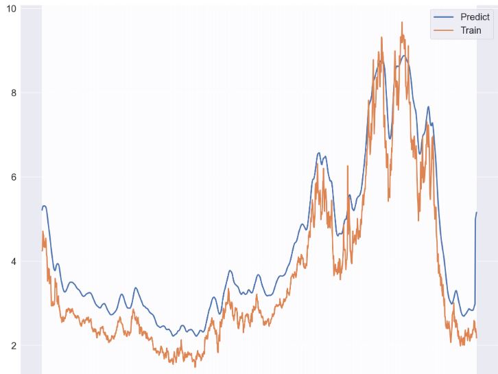
Let’s look at the test vs train NG data
dataset_total = pd.concat((train, test), axis = 0)
inputs = dataset_total[len(dataset_total) - len(test)- slot:].values
inputs = inputs.reshape(-1, 1)
x_test = []
y_test = []
for i in range (slot, len(test)+slot): #Test+15
x_test.append(inputs[i-slot:i, 0])
y_test.append(train.iloc[i, 0])
x_test, y_test = np.array(x_test), np.array(y_test)
x_test = np.reshape(x_test, (x_test.shape[0], x_test.shape[1], 1))
pred_price = lstm_model.predict(x_test)
b = pd.DataFrame(pred_price)
b.rename(columns = {0: 'gp_pred'}, inplace = True);
b.index = test.index
test_compare = pd.concat([test, b], 1)
plt.figure(figsize = (15,5))
plt.plot(test_compare['close'], color = 'red', label = "Actual Natural Gas Price")
plt.plot(test_compare['gp_pred'], color = 'blue', label = 'Predicted Price')
plt.title("Natural Gas Price Prediction On Test Data")
plt.xlabel('Time')
plt.ylabel('Natural gas price')
plt.legend(loc = 'best')
plt.show()
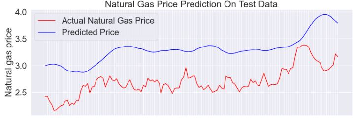
Model Loss
plt.plot(history.history['loss'])
plt.title('model loss')
plt.ylabel('loss')
plt.xlabel('epoch')
plt.legend(['train'], loc='upper right')
plt.show()

MSE and R2 score train vs test comparison
mse_train = mean_squared_error(train_compare['close'], train_compare['gp_pred'])
mse_test = mean_squared_error(test_compare['close'], test_compare['gp_pred'])
r2_train = r2_score(train_compare['close'], train_compare['gp_pred'])
r2_test = r2_score(test_compare['close'], test_compare['gp_pred'])
print("Train Data:\nMSE: {}\nR Square: {}".format(mse_train, r2_train))
print("\nTest Data:\nMSE: {}\nR Square: {}".format(mse_test, r2_test))
Train Data:
MSE: 0.6802612246761317
R Square: 0.8114795369678363
Test Data:
MSE: 0.39710431831336973
R Square: -5.03561417901034
- Let’s discuss the historical NG gas price prediction using LSTM Keras Sequential
%matplotlib inline
import numpy as np
import pandas as pd
import tensorflow as tf
from keras.utils.vis_utils import plot_model
import matplotlib.pyplot as plt
import plotly.express as px
import plotly.graph_objects as go
from plotly.subplots import make_subplots
print(tf.__version__)
2.10.0
Reading the input dataset
df = pd.read_csv('daily_csv.csv', parse_dates=["Date"])
len(df)
5953
#make dates the index
df.set_index(pd.DatetimeIndex(df.Date), inplace=True)
#fill date gaps
df = df.resample('D').pad()
#fix the Date column
df.Date = df.index.values
len(df)
8639
indexNames = df[ df['Price'] < 0 ].index
df.drop(indexNames , inplace=True)
df.shape
time_step = [i for i in range(df.shape[0])]
temps = df[['Price']]
series = np.array(temps)
time = np.array(time_step)
ig = px.line(df, x = 'Date', y = "Price", title = "Natural Gas Price")
fig.update_xaxes(nticks = 35)
fig.update_xaxes(tickangle=90)
fig.show()

Data preparation for LSTM
split_time = 7000
time_train = time[:split_time]
x_train = series[:split_time]
x_label_train = df[['Date']][:split_time]
time_valid = time[split_time:]
x_valid = series[split_time:]
x_label_valid = df[['Date']][split_time:]
window_size = 30
batch_size = 32
shuffle_buffer_size = 1000
def plot_series(time, series, format = "-", start = 0, end = None):
plt.plot(time[start:end], series[start:end], format)
plt.xlabel("Time")
plt.ylabel("Price")
plt.grid(True)
def windowed_dataset(series, window_size, batch_size, shuffle_buffer):
series = tf.expand_dims(series, axis = -1)
ds = tf.data.Dataset.from_tensor_slices(series)
ds = ds.window(window_size + 1, shift = 1, drop_remainder = True)
ds = ds.flat_map(lambda w: w.batch(window_size + 1))
ds = ds.shuffle(shuffle_buffer)
ds = ds.map(lambda w: (w[:-1], w[1:]))
return ds.batch(batch_size).prefetch(1)
def model_forecast(model, series, window_size):
ds = tf.data.Dataset.from_tensor_slices(series)
ds = ds.window(window_size, shift = 1, drop_remainder = True)
ds = ds.flat_map(lambda w: w.batch(window_size))
ds = ds.batch(32).prefetch(1)
forecast = model.predict(ds)
return forecast
tf.keras.backend.clear_session()
tf.random.set_seed(51)
np.random.seed(51)
window_size = 64
batch_size = 256
train_set = windowed_dataset(x_train, window_size, batch_size, shuffle_buffer_size)
print(train_set)
print(x_train.shape)
model = tf.keras.models.Sequential([
tf.keras.layers.Conv1D(filters = 32, kernel_size = 5,
strides = 1, padding = "causal",
activation = "relu",
input_shape = [None, 1]),
tf.keras.layers.LSTM(64, return_sequences = True),
tf.keras.layers.LSTM(64, return_sequences = True),
tf.keras.layers.Dense(30, activation = "relu"),
tf.keras.layers.Dense(10, activation = "relu"),
tf.keras.layers.Dense(1),
tf.keras.layers.Lambda(lambda x: x * 400)
])
lr_schedule = tf.keras.callbacks.LearningRateScheduler(
lambda epoch: 1e-8 * 10 ** (epoch / 20))
optimizer = tf.keras.optimizers.SGD(learning_rate = 1e-8, momentum = 0.9)
model.compile(loss = tf.keras.losses.Huber(),
optimizer = optimizer,
metrics = ["mae"])
history_1 = model.fit(train_set, epochs=70, callbacks = [lr_schedule])
fig = make_subplots(rows=2, cols=1, start_cell="top-left")
fig.add_trace(go.Scatter(x = history_1.history["lr"], y = history_1.history["loss"], name = 'loss'),
row = 1, col = 1, )
fig.add_trace(go.Scatter(x = history_1.history["lr"], y = history_1.history["mae"], name = 'mae'),
row = 2, col = 1)
fig.update_xaxes(title_text="Learning Rate", type="log", tickformat='.1e', row = 1, col = 1)
fig.update_yaxes(title_text="Loss", row = 1, col = 1)
fig.update_xaxes(title_text="Learning Rate", type="log", tickformat='.1e', row = 2, col = 1)
fig.update_yaxes(title_text="MAE", row = 2, col = 1)
fig.update_layout(
height = 800,
title_text = 'Training curve for mean squared error (mse) and loss '
)
fig.show()
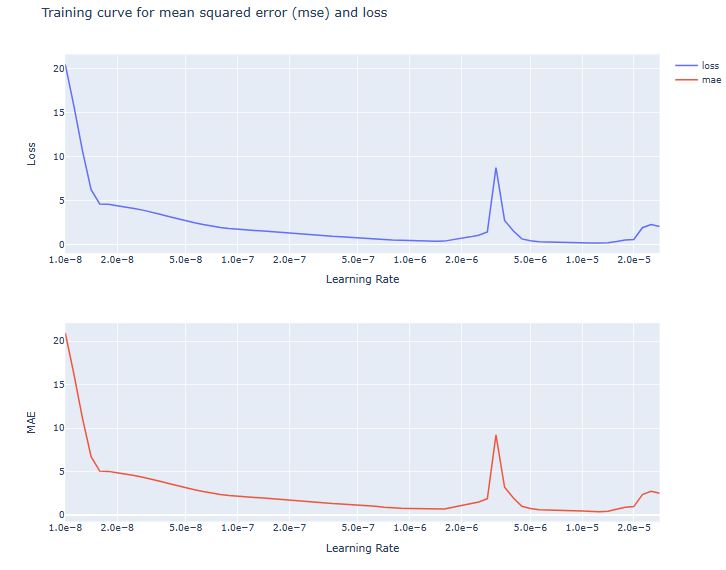
Finding the optimal learning rate
min_loss = min(history_1.history["loss"])
index = np.argmin(history_1.history["loss"])
learning_rate = history_1.history["lr"][index]
print(learning_rate)
1.2589254e-05
Building the LSTM model
def build_model():
model = tf.keras.models.Sequential([
tf.keras.layers.Conv1D(filters = 60, kernel_size = 5,
strides = 1, padding = "causal",
activation = "relu",
input_shape = [None, 1]),
tf.keras.layers.LSTM(60, return_sequences = True),
tf.keras.layers.LSTM(60, return_sequences = True),
tf.keras.layers.Dense(30, activation = "relu"),
tf.keras.layers.Dense(10, activation = "relu"),
tf.keras.layers.Dense(1),
tf.keras.layers.Lambda(lambda x: x * 400)
])
optimizer = tf.keras.optimizers.SGD(learning_rate = learning_rate, momentum = 0.9)
model.compile(loss = tf.keras.losses.Huber(),
optimizer = optimizer,
metrics = ["mae"])
return model
epochs = 250
model = build_model()
history_2 = model.fit(train_set, epochs = epochs)
plot_model(model, to_file = 'model_plot.png', show_shapes = True, show_layer_names = True)
Applying the LSTM model forecast
rnn_forecast = model_forecast(model, series[..., np.newaxis], window_size)
rnn_forecast = rnn_forecast[split_time - window_size:-1, -1, 0]
plt.figure(figsize = (18, 6))
plt.rcParams.update({'font.size': 18})
plot_series(time_valid, x_valid)
plot_series(time_valid, rnn_forecast)
plt.legend(['truth', 'forecast'], loc = 'upper right')

Plotting the training curve for mae and loss
zoom_begin = epochs - 50
zoon_end = epochs + 1
x_last = list(range(zoom_begin, zoon_end))
fig = make_subplots(rows = 2, cols = 2, start_cell = "top-left")
fig.add_trace(go.Scatter(y = history_2.history["mae"], name = 'mae'), row = 1, col = 1)
fig.update_xaxes(title_text="Epoch", type="log", row = 1, col = 1)
fig.update_yaxes(title_text="MAE", row = 1, col = 1)
fig.add_trace(go.Scatter(x = x_last, y = history_2.history["mae"][zoom_begin:], name = 'mae last 50 epochs'), row = 1, col = 2)
fig.update_xaxes(title_text="Epoch", type="log", row = 1, col = 2)
fig.update_yaxes(title_text="MAE", row = 1, col = 2)
fig.add_trace(go.Scatter(y = history_2.history["loss"], name='loss'), row = 2, col = 1)
fig.update_xaxes(title_text="Epoch", type="log", row = 2, col = 1)
fig.update_yaxes(title_text="Loss", row = 2, col = 1)
fig.add_trace(go.Scatter(x = x_last, y = history_2.history["loss"][zoom_begin:], name = 'loss last 50 epochs'), row = 2, col = 2)
fig.update_xaxes(title_text="Epoch", type="log", row = 2, col = 2)
fig.update_yaxes(title_text="Loss", row = 2, col = 2)
fig.update_layout(height = 800, title_text = 'Training curve for mae and loss ')
fig.show()
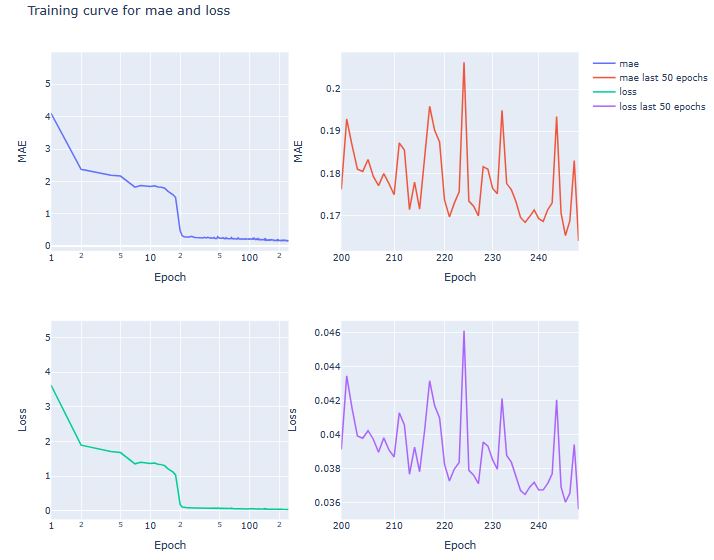
META Stock Isolation Forest Anomalies
- In this section, we will focus on detecting anomalies of time series of META stock returns in 2023 using the Isolation Forest algorithm.
- Reading the stock data
import yfinance as yf
import pandas as pd
ticker = 'META'
start_date = '2023-01-01'
end_date = '2023-10-30'
stock_data = yf.download(ticker, start=start_date, end=end_date)['Adj Close']
- Preparing the data
# Create an empity dataframe
returns = pd.DataFrame()
# Define the column Returns
returns['Returns'] = stock_data.pct_change()
from sklearn.preprocessing import StandardScaler
scaler = StandardScaler()
returns['Returns'] = scaler.fit_transform(returns['Returns'].values.reshape(-1,1))
data=returns.dropna()
data.tail()
Returns
Date
2023-10-23 0.478265
2023-10-24 -0.343518
2023-10-25 -1.724914
2023-10-26 -1.563206
2023-10-27 0.914842
- Applying the anomaly detection algorithm
from sklearn.ensemble import IsolationForest
model = IsolationForest(contamination=0.05)
model.fit(data[['Returns']])
# Predicting anomalies
data['Anomaly'] = model.predict(data[['Returns']])
data['Anomaly'] = data['Anomaly'].map({1: 0, -1: 1})
- META stock returns with anomalies detected by the Isolation Forest algorithm
# Ploting the results
plt.figure(figsize=(20,5))
plt.plot(data.index, data['Returns'], label='Returns')
plt.scatter(data[data['Anomaly'] == 1].index, data[data['Anomaly'] == 1]['Returns'], color='red')
plt.legend(['Returns', 'Anomaly'])
SMALL_SIZE = 18
MEDIUM_SIZE = 18
BIGGER_SIZE = 18
plt.rc('font', size=SMALL_SIZE) # controls default text sizes
plt.rc('axes', titlesize=SMALL_SIZE) # fontsize of the axes title
plt.rc('axes', labelsize=MEDIUM_SIZE) # fontsize of the x and y labels
plt.rc('xtick', labelsize=SMALL_SIZE) # fontsize of the tick labels
plt.rc('ytick', labelsize=SMALL_SIZE) # fontsize of the tick labels
plt.rc('legend', fontsize=SMALL_SIZE) # legend fontsize
plt.rc('figure', titlesize=BIGGER_SIZE) # fontsize of the figure title
plt.grid()
plt.show()
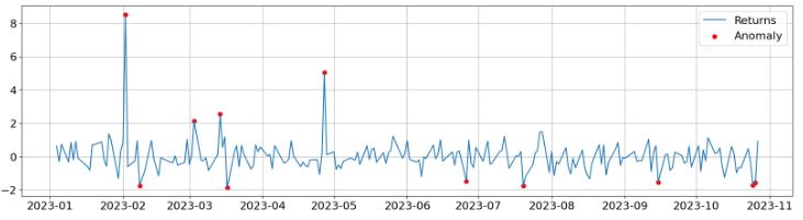
S&P 500 Historical Price Anomalies
- In this section, we will detect volatility anomalies in the S&P500 index dataset.
- Reading the input data
import os
os.chdir('YOURPATH')
os. getcwd()
df = pd.read_csv('S&P_500_Index_Data.csv', parse_dates=['date'])
- Plotting the input data
df0=df.copy()
fig = go.Figure()
fig.add_trace(go.Scatter(x=df0.date, y=df0.close,
mode='lines',
name='close'))
fig.update_layout(showlegend=True)
fig.update_layout(
title="S&P 500 Close Price USD",
xaxis_title="Date",
yaxis_title="Close Price USD",
legend_title="",
font=dict(
family="Courier New, monospace",
size=18,
color="RebeccaPurple"
)
)
fig.show()

#To model returns we will use daily % change
daily = df["close"].pct_change()
daily.dropna(inplace = True)
#Resample returns per month and take STD as measure of volatility
mnthly_annu = daily.resample("M").std()*np.sqrt(12) #number of periods = 12
- Plotting the monthly annualized volatility with 2 anomalies
#Visulize major market events that show up in the volatility
import matplotlib.patches as mpatches
plt.rcParams.update({'font.size': 18})
plt.plot(mnthly_annu,lw=3)
plt.axvspan('1987','1989',color='r',alpha=.5)
plt.axvspan('2008','2010',color='r',alpha=.5)
plt.title("Monthly Annualized volatility")
labs = mpatches.Patch(color='red',alpha=.5, label="Black Monday & '08 Crash")
plt.legend(handles=[labs])
plt.grid(color = 'black', linestyle = '--', linewidth = 1.0)

- Plotting monthly volatility ranking
#for each year rank each month based on volatility
ranked = mnthly_annu.groupby(mnthly_annu.index.year).rank()
#average the ranks over all years for each month
final = ranked.groupby(ranked.index.month).mean()
#plot results for ranked S&P 500 volatility with mean of final.mean()
b_plot = plt.bar(x = final.index, height = final)
b_plot[9].set_color("g")
b_plot[11].set_color("r")
for i, v in enumerate(round(final,2)):
plt.text(i+.8, 1, str(v), color = "black", fontweight = "bold")
plt.axhline(final.mean(), ls = "--", color = "k", label = round(final.mean(),2))
plt.title("Average Monthly Volatility Ranking S&P500 since 1986")
plt.legend()
plt.show()

Summary
- In this post, we have addressed the stock portfolio optimization problem based upon the 5 pillars of (fintech) time series analysis

- Portfolio 1 Stock Risk/Return Ranking

- Problem: Sales volumes for META, AMZN, and AAPL have been falling since 2022.
- Portfolio 2 benchmark portfolio = tsla_df*0.25 + dis_df* 0.25+aapl_df*0.25+amd_df* 0.25,
- new_weights = [0.65871, 0.34129]
- optimized portfolio = tsla_df* new_weights[0] + aapl_df* new_weights[1]
- Sharpe Ratio for AAPL: 0.82
- Sharpe Ratio for TSLA: 1.11
- Sharpe Ratio for DIS: -0.26
- Sharpe Ratio for AMD: 0.63
- Apple’s Standard Deviation: 0.021520708530783472
- Tesla’s Standard Deviation: 0.043479817357367966
- Disney’s Standard Deviation: 0.02271810742856512
- AMD’s Standard Deviation: 0.03403554120470168
- Visualizing the annualized expected returns mu
- aapl 0.241023
- tsla 0.676460
- dis -0.149894
- amd 0.184567
- Visualizing the covariance matrix S
aapl tsla nvda meta
aapl 0.116819 0.121311 0.126178 0.098940
tsla 0.121311 0.477221 0.200507 0.120923
nvda 0.126178 0.200507 0.303958 0.148242
meta 0.098940 0.120923 0.148242 0.226365
- Fitting linear relation among stock returns and ^GSPC Benchmark
AAPL beta: [1.194] AAPL alpha: [0.001]
TSLA beta: [1.516] TSLA alpha: [0.002]
DIS beta: [1.075] DIS alpha: [-0.001]
AMD beta: [1.508] AMD alpha: [0.001]
Performance Metrics
Strategy Benchmark
------------------------- ---------- -----------
Start Period 2020-01-02 2020-01-02
End Period 2023-10-26 2023-10-26
Risk-Free Rate 0.0% 0.0%
Time in Market 100.0% 100.0%
Cumulative Return 338.55% 82.5%
CAGR﹪ 47.31% 17.07%
Sharpe 0.99 0.6
Prob. Sharpe Ratio 97.28% 87.8%
Smart Sharpe 0.94 0.57
Sortino 1.45 0.85
Smart Sortino 1.38 0.81
Sortino/√2 1.02 0.6
Smart Sortino/√2 0.98 0.57
Omega 1.19 1.19
Max Drawdown -65.0% -56.61%
Longest DD Days 660 660
Volatility (ann.) 53.88% 39.1%
R^2 0.86 0.86
Information Ratio 0.08 0.08
Calmar 0.73 0.3
Skew -0.13 -0.24
Kurtosis 2.21 2.38
Expected Daily % 0.15% 0.06%
Expected Monthly % 3.27% 1.32%
Expected Yearly % 44.71% 16.23%
Kelly Criterion 7.65% 4.69%
Risk of Ruin 0.0% 0.0%
Daily Value-at-Risk -5.37% -3.96%
Expected Shortfall (cVaR) -5.37% -3.96%
Max Consecutive Wins 13 11
Max Consecutive Losses 8 8
Gain/Pain Ratio 0.19 0.11
Gain/Pain (1M) 0.97 0.53
Payoff Ratio 1.01 0.93
Profit Factor 1.19 1.11
Common Sense Ratio 1.25 1.08
CPC Index 0.64 0.56
Tail Ratio 1.05 0.97
Outlier Win Ratio 3.0 4.24
Outlier Loss Ratio 3.15 4.11
MTD -13.78% -9.78%
3M -20.04% -16.91%
6M 19.14% 7.97%
YTD 53.63% 35.1%
1Y -2.88% 1.19%
3Y (ann.) 5.44% 0.3%
5Y (ann.) 47.31% 17.07%
10Y (ann.) 47.31% 17.07%
All-time (ann.) 47.31% 17.07%
Best Day 15.9% 12.86%
Worst Day -16.67% -12.25%
Best Month 55.18% 30.87%
Worst Month -29.83% -21.91%
Best Year 354.51% 113.44%
Worst Year -57.1% -51.11%
Avg. Drawdown -10.07% -7.7%
Avg. Drawdown Days 50 51
Recovery Factor 5.21 1.46
Ulcer Index 0.28 0.25
Serenity Index 0.85 0.18
Avg. Up Month 19.01% 11.77%
Avg. Down Month -10.16% -7.98%
Win Days % 53.69% 54.01%
Win Month % 52.17% 50.0%
Win Quarter % 68.75% 56.25%
Win Year % 75.0% 75.0%
Beta 1.27 -
Alpha 0.23 -
Correlation 92.49% -
Treynor Ratio 265.64% -
5 Worst Drawdowns
Start Valley End Days Max Drawdown 99% Max Drawdown
1 2022-01-04 2023-01-03 2023-10-26 660 -65.004995 -63.523622
2 2020-02-20 2020-03-18 2020-06-08 109 -45.840571 -43.836799
3 2021-01-27 2021-03-08 2021-10-21 267 -32.740417 -30.820440
4 2020-09-01 2020-09-08 2020-11-23 83 -27.738370 -21.804801
5 2021-11-05 2021-12-20 2022-01-03 59 -20.570677 -18.460889
- Portfolio 2 cumulative return: 2% before PO and 6% after PO
- NVDA SMA 50-100 Entry/Exit Trading Strategy
index Backtest
-------------------------------
0 Annual Return 1.01
1 Cumulative Returns 19.48
2 Annual Volatility 0.66
3 Sharpe Ratio 1.53
4 Sortino Ratio 2.47
- NVDA Fundamental Analysis against Peers:
- Overall NVDA gets a fundamental rating of 7 out of 10.
- The Altman-Z score of NVDA (29.91) is better than 95.24% of its industry peers.
- NVDA has a better Debt to FCF ratio (0.94) than 77.14% of its industry peers.
- NVDA‘s Current ratio of 2.79 is in line compared to the rest of the industry. NVDA outperforms 41.90% of its industry peers.
- In the last year, the EPS has been growing by 20.41%, which is quite impressive.
- The EPS will grow by 54.68% on average per year.
- NVDA is valuated quite expensively with a Price/Earnings ratio of 77.68.
- The average S&P500 Price/Earnings ratio is at 22.86. NVDA is valued rather expensively when compared to this.
- 68.57% of the companies in the same industry are cheaper than NVDA, based on the Enterprise Value to EBITDA ratio.
- The excellent profitability rating of NVDA may justify a higher PE ratio.
- NVDA has a yearly dividend return of 0.04%, which is pretty low.
- The dividend of NVDA has a limited annual growth rate of 2.26%.
- AAPL Price LSTM Forecasting rmse = 5.9636350262044076, loss: 0.0081
- Portfolio 3: (a) [‘TATAMOTORS’,’DABUR’, ‘ICICIBANK’,’WIPRO’,’INFY’], (b) [‘AXISBANK’, ‘HDFCBANK’, ‘ICICIBANK’, ‘KOTAKBANK’, ‘SBIN’]
- Portfolio 3a optimization:
TATAMOTORS 83%
ICICBANK 14%
Others* 3%
* DABUR, WIPRO, INFY
Average Daily returns(%) of stocks in your portfolio
TATAMOTORS -0.026735
DABUR 0.008902
ICICIBANK 0.031856
WIPRO -0.132460
INFY -0.033956
Annualized Standard Deviation (Volatility(%), 252 trading days) of individual stocks in your portfolio on the basis of daily simple returns.
TATAMOTORS 35.808329
DABUR 23.661057
ICICIBANK 23.140343
WIPRO 25.312352
INFY 27.060286
- Portfolio 3b:
print (df_returns.mean())
AXISBANK 0.000463
HDFCBANK 0.000314
ICICIBANK 0.000319
KOTAKBANK -0.000279
SBIN 0.000052
Portfolio 0.000174
print(sharpe_ratio)
[0.31098709022009735]
- TATAMOTORS Historical Data
╒════════════════╤═════════╤══════════════════════╤═════════╕
│ │ Mean │ Standard Deviation │ VaR % │
╞════════════════╪═════════╪══════════════════════╪═════════╡
│ ['TATAMOTORS'] │ -0.0003 │ 0.0226 │ -0.0393 │
╘════════════════╧═════════╧══════════════════════╧═════════╛
The Bootstrap VaR measure is -0.03675094394004405
The VAR of stock using decay factor is -0.012218757045694294
The mean Monte Carlo VaR is -0.03722746593892233
- We have conducted a series of statistical experiments to check stationarity in BTC-USD time series. Our tests have shown that the crypto price is following an up-trend, meaning the time-series price data is non-stationary. We observed that BTC-USD prices became stationary only after calculating differences.
- The BTC-USD seasonal decomposition suggests that crypto price movements follow specific sequences that are independent of other assets.
- Although different fluctuating degree can be seen by years 2020-23, generally it can be stated that Bitcoin prices are highly volatile.
- We have compared the accuracy of BTC-USD 2020-23 price prediction using Long Short Term Memory (LSTM) TensorFlow Keras NN and statistical (ARIMA/SARIMA/SARIMAX) model.
- Although both ARIMA and LSTM could perform well in predicting BTC-USD price, taking less historical data to make prediction in LSTM could lead to better results. On the other hand, ARIMA is quite efficient in making only short-term predictions, and the outcome is very sensitive to the time interval.
- We have demonstrated that time series forecasting is a reliable technique in NG price predictions. The Dickey-Fuller Test (DFT) with a 95% confidence interval revealed that the NG price time series is non-stationary, which is due to the trend. Two ways to make a series stationary were detrending and differencing. RNNs don’t require a series to be stationary. The parameters for the (S)AR(I)MA model were tuned using the ACF and PACF plots. The Normal Q-Q plot provided an indication of univariate normality of the NG dataset. Both ARIMA and RNN LSTM models can be effective for a collection of historical NG data, exhibiting a degree of predictable behavior.
- Finally, these are 5 simple QT-powered ways to balance your portfolio in terms of min (Risk/Return) ratio:
- Portfolio Diversification using stock correlation/similarity metrics and Alpha/Beta relative to a benchmark.
- Stochastic Portfolio Optimization using the Sharpe Ratio (Efficiency Curve), VAR, Bootstrap, Decay, and Monte Carlo
- Maximizing Risk-Adjusted Returns using the Sharpe Ratio, the simulated portfolio returns with backtesting against a benchmark, and comparing (daily, monthly, EOY and cumulative) returns and their quantiles
- Minimizing Risk Exposure using sales volumes, stock elasticity (STD), rolling 6-months metrics (Beta, Sharpe, Sortino, and volatility), worst drawdowns, underwater plots, statistical testing, simulated VAR, and basic descriptive statistics (variance, skewness, and kurtosis)
- Robust automated stock screening and short-term time series forecasting by integrating technical trading indicators (TTIs), (unsupervised/supervised and deep learning) ML/AI algorithms, and fundamental analysis.
- And here is the 10-step road ahead:
- The identified assets will be consolidated into a virtual portfolio for subsequent QT performance tracking. Their future returns will be benchmarked against the S&P 500 index, serving as a comparative standard.
- Create an automated QT platform and deploy it via an open-source app framework for traders and investors alike.
- Explore various scenario-specific ideas of anomaly detection in fintech time series to better understand the validity range.
- Implement the automated identification of undervalued stocks based upon a rigorous fundamental analysis of financial indicators that reflect a company’s operational efficiency, liquidity, profitability, and market valuation.
- Develop and integrated time series forecasting framework based upon statistical ARIMA-type models, Prophet, stochastic simulations (e.g. Monte Carlo), and TensorFlow deep learning such as LSTM Keras.
- Continue exploring portfolio diversification ideas linked to tech stocks, commodities, and crypto.
- Examine a diversified crypto portfolio. It may include tokens that span industry sectors such as gaming, file storage, environmental protection, and finance. Expand across geographies to include tokens that are primarily used within specific geographic regions.
- A flagship pilot study will investigate whether commodities yield diversification benefits to stock portfolios for loss-averse investors using a sample of 10+ individual futures contracts and one index of commodity futures.
- Perform a comprehensive stock market research and sentiment analysis using web data mining.
- Develop verification strategies for establishing reliability and validity in QT deliverables against 3rd party SaaS products and industry peers.
References
- Stock Market Analysis + Prediction using LSTM
- Anomaly Detection
- Anomaly-Detection-in-Time-Series Data using LSTM in Keras
- How To Build Capital Asset Pricing Model (CAPM) Using Python
- Trading Dashboard with Yfinance & Python
- The Science of Smart Investing: Portfolio Evaluation with Python
- Time-Series Forecasting: Predicting Apple Stock Price Using An LSTM Model
- How to build a financial portfolio using Python
- Portfolio with Sharpe Ratio
- Risk management VAR
- Using Fundamental Analysis to Identify Undervalued Stocks
- Cryptocurrency Price Prediction using ARIMA Model
- Bitcoin price prediction using ARIMA and LSTM
- How to Run Stationarity Tests on Cryptocurrencies Trading Data
- Time Series forecasting of natural gas prices with Python
- FMP
- Natural gas price prediction
- Natural Gas Price Prediction using Time Series
- Forecasting of Energy Data using Exponential smoothing, ARIMA and LSTMs.
Explore More
- Robust Anomaly Detection using the Isolation Forest Algorithm: Financial Transactions vs NYC Taxi Rides
- Returns-Volatility Domain K-Means Clustering and LSTM Anomaly Detection of S&P 500 Stocks
- Real-Time Anomaly Detection of NAB Ambient Temperature Readings using the TensorFlow/Keras Autoencoder
- Optimizing NVIDIA Returns-Drawdowns MVA Crossovers vs Simple RNN Mean Reversal Trading Strategies in Python
- Oracle Monte Carlo Stock Simulations
- Predicting Rolling Volatility of the NVIDIA Stock – GARCH vs XGBoost
- IQR-Based Log Price Volatility Ranking of Top 19 Blue Chips
- Multiple-Criteria Technical Analysis of Blue Chips in Python
- Blue-Chip Stock Portfolios for Quant Traders
- Time Series Forecasting of Hourly U.S.A. Energy Consumption – PJM East Electricity Grid
- Working with FRED API in Python: U.S. Recession Forecast & Beyond
- Eric Marsden’s Top 6 Reliability/Risk Engineering Learnings
- Risk-Return Analysis and LSTM Price Predictions of 4 Major Tech Stocks in 2023
- SARIMAX X-Validation of EIA Crude Oil Prices Forecast in 2023 – 2. Brent
- BTC-USD Freefall vs FB/Meta Prophet 2022-23 Predictions
- BTC-USD Price Prediction with LSTM
- Stock Portfolio Risk/Return Optimization
- Quant Trading using Monte Carlo Predictions and 62 AI-Assisted Trading Technical Indicators (TTI)
- Are Blue Chips Perfect for This Bear Market?
- Bear Market Similarity Analysis using Nasdaq 100 Index Data
- S&P 500 Algorithmic Trading with FBProphet
- Stock Forecasting with FBProphet
- Short-Term Stock Market Price Prediction using Deep Learning Models
- The Donchian Channel vs Buy-and-Hold Breakout Trading Systems – $MO Use-Case
- Portfolio max(Return/Risk) Stochastic Optimization of 20 Dividend Growth Stocks
- 360-Deg Revision of Risk Aware Investing after SVB Collapse – 1. The Financial Sector
- Applying a Risk-Aware Portfolio Rebalancing Strategy to ETF, Energy, Pharma, and Aerospace/Defense Stocks in 2023
- Predicting the JPM Stock Price and Breakouts with Auto ARIMA, FFT, LSTM and Technical Trading Indicators
- Deep Reinforcement Learning (DRL) on $MO 8.07% DIV USA Stock Data 2022-23
- Advanced Integrated Data Visualization (AIDV) in Python – 1. Stock Technical Indicators
Appendix A: Stock Risk Class
class StockRisk:
def __init__(self, start_date, end_date, investment: int, ticker: str, iterations:int):
"""Initialization
Args:
start_date (Date): Indicates the date from which the stock data will be extracted
end_date (Date): Indicates the date till which the stock data will be extracted. In this case it is today
investment (int): The initial investment value
ticker (str): The name of the stock
"""
self.start_date = start_date
self.end_date = end_date
self.investment = investment
self.ticker = ticker
self.iterations = iterations
def var_historical(self):
try:
returns = df_returns.copy()
#returns = df_returns.copy()
# check for variance
var_stock = returns.var()
# Calculate mean returns of the stock
avg_rets = returns.mean()
# Calculate SD of the stock
avg_std = returns.std()
returns['Stock'].mean()
returns['Stock'].median()
returns['Stock'].quantile(.05, 'lower')
# var_hist = returns['Stock'].quantile(.05, 'lower')
returns.sort_values('Stock').head(13)
var_hist = np.percentile(returns['Stock'], 5, interpolation = 'lower')
print(tabulate([[self.ticker,avg_rets,avg_std,var_hist]],
headers = ['Mean', 'Standard Deviation', 'VaR %'],
tablefmt = 'fancy_grid',stralign='center',numalign='center',floatfmt=".4f"))
print(var_hist)
return var_hist
except Exception as e:
print(f'An exception occurred while executing var_weighted_decay_factor: {e}')
def var_bootstrap(self):
"""Bootstrap
Args:
iterations (int): The number of times the resampling is carried out
"""
def var_boot(data):
dff = pd.DataFrame(data, columns = ['sample'])
return np.percentile(dff, 5, interpolation = 'lower')
# return dff['sample'].quantile(.05, 'lower')
def bootstrap(data, func):
sample = np.random.choice(data, len(data))
return func(sample)
def generate_sample_data(data, func, size):
bs_replicates = np.empty(size)
for i in range(size):
bs_replicates[i] = bootstrap(data, func)
return bs_replicates
#returns = df_returns.copy()
returns = df_returns.copy()
bootstrap_VaR = generate_sample_data(returns['Stock'], var_boot, self.iterations)
var_bootstrap = np.mean(bootstrap_VaR)
print(f'The Bootstrap VaR measure is {np.mean(bootstrap_VaR)}')
return np.mean(bootstrap_VaR)
def var_weighted_decay_factor(self):
try:
#returns = df_returns.copy()
returns = df_returns.copy()
decay_factor = 0.5 #we’re picking this arbitrarily
n = len(returns)
wts = [(decay_factor**(i-1) * (1-decay_factor))/(1-decay_factor**n) for i in range(1, n+1)]
#Need to reverse the PnL to put recent returns on top
returns_recent_first = returns[::-1]
weights_dict = {'Returns':returns_recent_first, 'Weights':wts}
wts_returns = pd.DataFrame(returns_recent_first['Stock'])
wts_returns['wts'] = wts
sort_wts = wts_returns.sort_values(by='Stock')
sort_wts['Cumulative'] = sort_wts.wts.cumsum()
sort_wts
#Find where cumulative (percentile) hits 0.05
sort_wts = sort_wts.reset_index()
idx = sort_wts[sort_wts.Cumulative <= 0.05].Stock.idxmax()
sort_wts.filter(items = [idx], axis = 0)
xp = sort_wts.loc[idx:idx+1, 'Cumulative'].values
fp = sort_wts.loc[idx:idx+1, 'Stock'].values
var_decay = np.interp(0.05, xp, fp)
print(f'The VAR of stock using decay factor is {var_decay} ')
return var_decay
except Exception as e:
print(f'An exception occurred while executing var_weighted_decay_factor: {e}')
def var_monte_carlo(self):
try:
returns = df_returns.copy()
returns_mean = returns['Stock'].mean()
returns_sd = returns['Stock'].std()
def simulate_values(mu, sigma):
try:
result = []
for i in range(self.iterations):
tmp_val = np.random.normal(mu, sigma, (len(returns)))
var_MC = np.percentile(tmp_val, 5, interpolation = 'lower')
result.append(var_MC)
return result
except Exception as e:
print(f'An exception occurred while generating simulation values: {e}')
sim_val = simulate_values(returns_mean,returns_sd)
tmp_df = pd.DataFrame(columns=['Iteration', 'VaR'])
tmp_df['Iteration'] = [i for i in range(1,self.iterations +1)]
tmp_df['VaR'] = sim_val
VaR_MC = statistics.mean(sim_val)
print(f'The mean Monte carlo VaR is {VaR_MC}')
return VaR_MC
except Exception as e:
print(f'An exception occurred while executing var_monte_carlo: {e}')
def show_summary(self):
try:
var_hist = self.var_historical()
var_bs = self.var_bootstrap()
var_decay = self.var_weighted_decay_factor()
var_MC = self.var_monte_carlo()
print(tabulate([[self.ticker,var_hist,var_bs,var_decay, var_MC]],
headers = ['Historical', 'Bootstrap', 'Decay', 'Monte Carlo'],
tablefmt = 'fancy_grid',stralign='center',numalign='center',floatfmt=".4f"))
except Exception as e:
print(f'An exception occurred while executing show_summary: {e}')
def plot_stock_price(self):
try:
stock_price = obj_loadData.df_stock_data.copy()
fig, ax = plt.subplots(figsize=(10, 5))
fig = sns.histplot(stock_price,color = 'blue',alpha = .2, bins = 50, kde = True)
return fig
except Exception as e:
print(f'An exception occurred while generating plot_stock_price: {e}')
def plot_stock_returns(self):
try:
returns = df_returns.copy()
fig, ax = plt.subplots(figsize=(10, 5))
fig = sns.histplot(returns,color = 'blue',alpha = .2, bins = 50, kde = True)
return fig
except Exception as e:
print(f'An exception occurred while generating plot_stock_returns: {e}')
def plot_shade(self, var_returns):
try:
returns = df_returns.copy()
fig, ax = plt.subplots(figsize=(10, 5))
sns.histplot(returns,color = 'blue',alpha = .2,bins = 50, kde = True)
plt.axvline(var_returns, 0, 25, color = 'red', alpha = .15)
plt.text(var_returns, 25, f'VAR {round(var_returns, 4)} @ 5%',
horizontalalignment='right',
size='small',
color='navy')
left, bottom, width, height = (var_returns, 0, -5, 30)
rect=mpatches.Rectangle((left,bottom),width,height,
fill=True,
color="red",
alpha=0.2,
facecolor="red",
linewidth=2)
plt.gca().add_patch(rect)
except Exception as e:
print(f'An exception occurred while generating plot_shade: {e}')
def plot_stock_returns_shaded(self, var_method):
try:
if var_method == 'historical':
self.plot_shade(self.var_historical())
elif var_method == 'bootstrap':
self.plot_shade(self.var_bootstrap())
elif var_method == 'monte_carlo':
self.plot_shade(self.var_monte_carlo())
else:
self.plot_shade(self.var_weighted_decay_factor())
except Exception as e:
print(f'An exception occurred while generating plot_stock_returns_shaded: {e}')


Make a one-time donation
Make a monthly donation
Make a yearly donation
Choose an amount
Or enter a custom amount
Your contribution is appreciated.
Your contribution is appreciated.
Your contribution is appreciated.
DonateDonate monthlyDonate yearly
Leave a comment