- The main objective of this post is to implement and validate time series anomaly detection using the Isolation Forest algorithm.
- Isolation Forest is an unsupervised algorithm for anomaly detection. It does not require a labeled time-series dataset to identify anomalies.
- The challenge is to develop robust anomaly detection models that can accurately distinguish between normal and abnormal data points, thereby assisting in fraud detection, fault diagnosis, and outlier identification.
- To address this challenge, we will consider two real-world datasets representing sequences of data points indexed in time order.
- The first dataset contains information about various financial transactions. Anomaly detection in transactions means identifying unusual or unexpected patterns within transactions or related activities.
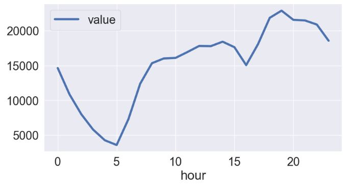
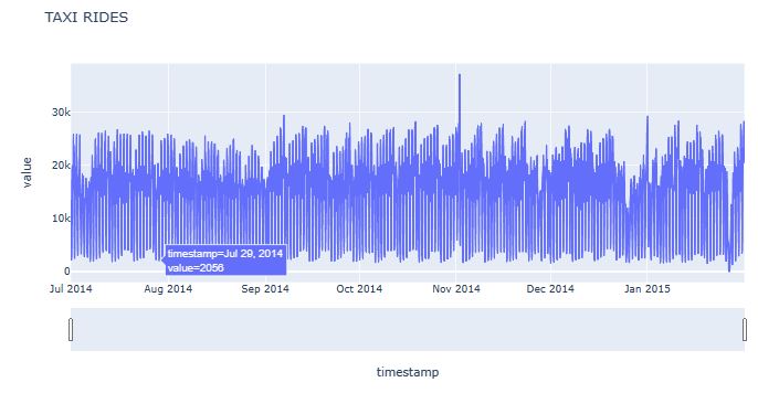
- The second dataset shows the number of NYC taxi rides for 6 months recorded in 30 min intervals. The raw data is from the NYC Taxi and Limousine Commission. The NYC taxi dataset is available as part of the Numenta anomaly benchmark here.
- Choosing and combining detection algorithms (detectors), feature engineering methods (transformers), and ensemble methods (aggregators) properly is the key to build an effective anomaly detection model.
Preparations
Let’s set the working directory YOURPATH
import os
os.chdir('YOURPATH')
os. getcwd()
and import the key libraries
import pandas as pd
import plotly.express as px
from sklearn.model_selection import train_test_split
from sklearn.ensemble import IsolationForest
from sklearn.metrics import classification_report
import matplotlib as mpl
import matplotlib.pyplot as plt
from datetime import datetime
Transactions
- Reading the input dataset
data = pd.read_csv("transaction_anomalies_dataset.csv")
print(data.head())
Transaction_ID  Transaction_Amount  Transaction_Volume  \
0            TX0         1024.835708                   3
1            TX1         1013.952065                   4
2            TX2          970.956093                   1
3            TX3         1040.822254                   2
4            TX4          998.777241                   1

   Average_Transaction_Amount  Frequency_of_Transactions  \
0                  997.234714                         12
1                 1020.210306                          7
2                  989.496604                          5
3                  969.522480                         16
4                 1007.111026                          7

   Time_Since_Last_Transaction Day_of_Week Time_of_Day  Age  Gender   Income  \
0                           29      Friday       06:00   36    Male  1436074
1                           22      Friday       01:00   41  Female   627069
2                           12     Tuesday       21:00   61    Male   786232
3                           28      Sunday       14:00   61    Male   619030
4                            7      Friday       08:00   56  Female   649457

  Account_Type
0      Savings
1      Savings
2      Savings
3      Savings
4      Savings
print(data.info())
<class 'pandas.core.frame.DataFrame'>
RangeIndex: 1000 entries, 0 to 999
Data columns (total 12 columns):
 #   Column                       Non-Null Count  Dtype
---  ------                       --------------  -----
 0   Transaction_ID               1000 non-null   object
 1   Transaction_Amount           1000 non-null   float64
 2   Transaction_Volume           1000 non-null   int64
 3   Average_Transaction_Amount   1000 non-null   float64
 4   Frequency_of_Transactions    1000 non-null   int64
 5   Time_Since_Last_Transaction  1000 non-null   int64
 6   Day_of_Week                  1000 non-null   object
 7   Time_of_Day                  1000 non-null   object
 8   Age                          1000 non-null   int64
 9   Gender                       1000 non-null   object
 10  Income                       1000 non-null   int64
 11  Account_Type                 1000 non-null   object
dtypes: float64(2), int64(5), object(5)
memory usage: 93.9+ KB
None
- Data preparation
# Calculate mean and standard deviation of Transaction Amount
mean_amount = data['Transaction_Amount'].mean()
std_amount = data['Transaction_Amount'].std()

# Define the anomaly threshold (2 standard deviations from the mean)
anomaly_threshold = mean_amount + 2 * std_amount

# Flag anomalies
data['Is_Anomaly'] = data['Transaction_Amount'] > anomaly_threshold

# Scatter plot of Transaction Amount with anomalies highlighted
fig_anomalies = px.scatter(data, x='Transaction_Amount', y='Average_Transaction_Amount',
                           color='Is_Anomaly', title='Anomalies in Transaction Amount')
fig_anomalies.update_traces(marker=dict(size=12),
                            selector=dict(mode='markers', marker_size=1))
fig_anomalies.show()

- Calculating the anomaly ratio
# Calculate the number of anomalies
num_anomalies = data['Is_Anomaly'].sum()

# Calculate the total number of instances in the dataset
total_instances = data.shape[0]

# Calculate the ratio of anomalies
anomaly_ratio = num_anomalies / total_instances
print(anomaly_ratio)
0.02
- Splitting the data into the features (X) and the target variable (y), train/test data splitting, training the model and predicting anomalies on the test dataset
relevant_features = ['Transaction_Amount',
                     'Average_Transaction_Amount',
                     'Frequency_of_Transactions']

# Split data into features (X) and target variable (y)
X = data[relevant_features]
y = data['Is_Anomaly']

# Split data into train and test sets
X_train, X_test, y_train, y_test = train_test_split(X, y, test_size=0.2, random_state=42)

# Train the Isolation Forest model
model = IsolationForest(contamination=0.02, random_state=42)
model.fit(X_train)
                    IsolationForest
IsolationForest(contamination=0.02, random_state=42)
# Predict anomalies on the test set
y_pred = model.predict(X_test)

# Convert predictions to binary values (0: normal, 1: anomaly)
y_pred_binary = [1 if pred == -1 else 0 for pred in y_pred]

# Evaluate the model's performance
report = classification_report(y_test, y_pred_binary, target_names=['Normal', 'Anomaly'])
print(report)
               precision    recall  f1-score   support

      Normal       1.00      1.00      1.00       196
     Anomaly       1.00      1.00      1.00         4

    accuracy                           1.00       200
   macro avg       1.00      1.00      1.00       200
weighted avg       1.00      1.00      1.00       200
# Relevant features used during training
relevant_features = ['Transaction_Amount', 'Average_Transaction_Amount', 'Frequency_of_Transactions']

# Get user inputs for features
user_inputs = []
for feature in relevant_features:
    user_input = float(input(f"Enter the value for '{feature}': "))
    user_inputs.append(user_input)

# Create a DataFrame from user inputs
user_df = pd.DataFrame([user_inputs], columns=relevant_features)

# Predict anomalies using the model
user_anomaly_pred = model.predict(user_df)

# Convert the prediction to binary value (0: normal, 1: anomaly)
user_anomaly_pred_binary = 1 if user_anomaly_pred == -1 else 0

if user_anomaly_pred_binary == 1:
    print("Anomaly detected: This transaction is flagged as an anomaly.")
else:
    print("No anomaly detected: This transaction is normal.")
Enter the value for 'Transaction_Amount': 1000
Enter the value for 'Average_Transaction_Amount': 1500
Enter the value for 'Frequency_of_Transactions': 12
No anomaly detected: This transaction is normal.
Enter the value for 'Transaction_Amount': 2000
Enter the value for 'Average_Transaction_Amount': 2300
Enter the value for 'Frequency_of_Transactions': 10
Anomaly detected: This transaction is flagged as an anomaly.
Taxi Rides
- Reading the input NYC taxi dataset
df = pd.read_csv('taxi_rides.csv')
- Data preparation
from datetime import datetime
df['timestamp']=pd.to_datetime(df['timestamp'])
df=df.set_index('timestamp').resample("H").mean().reset_index()
df['hour']=df.timestamp.dt.hour
df['weekday']=pd.Categorical(df.timestamp.dt.strftime('%A'), categories=['Monday','Tuesday','Wednesday','Thursday','Friday','Saturday', 'Sunday'], ordered=True)
- Data visualization
ax=df[['value','weekday']].groupby('weekday').mean().plot(figsize=(14, 5),lw=4)

df[['value','hour']].groupby('hour').mean().plot(figsize=(10, 5),lw=4)
import plotly.express as px
fig = px.line(df.reset_index(), x='timestamp', y='value', title='TAXI RIDES')
fig.update_xaxes(
    rangeslider_visible=True,
)
fig.show()
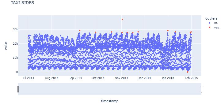
- Anomaly detection
from sklearn.ensemble import IsolationForest
model =  IsolationForest(contamination=0.004)
model.fit(df[['value']])
           IsolationForest
IsolationForest(contamination=0.004)
df['outliers']=pd.Series(model.predict(df[['value']])).apply(lambda x: 'yes' if (x == -1) else 'no' )
df.query('outliers=="yes"')
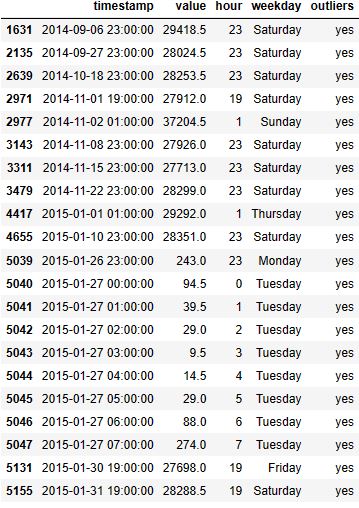
fig = px.scatter(df.reset_index(), x='timestamp', y='value', color='outliers', hover_data=['weekday'], title='TAXI RIDES')
fig.update_xaxes(
    rangeslider_visible=True,
)
fig.show()
Summary
- Results show that we can perform successful anomaly detection in financial transactions using the Isolation Forest algorithm. These anomalies represent patterns or outliers that indicate irregular or fraudulent behavior.
- We have also used the aforementioned algorithm to detect anomalies in the dataset containing the number of taxi passengers in New York. Our observations are generally consistent with earlier case studies and QC comparisons.
- Overall, the historical time series data can be used to predict anomalies in real time and give information about the nature of the anomalies to react well when they occur.
Explore More
- Advanced Integrated Data Visualization (AIDV) in Python – 2. Dabl Auto EDA & ML
- Unsupervised ML Clustering, Customer Segmentation, Cohort, Market Basket, Bank Churn, CRM, ABC & RFM Analysis – A Comprehensive Guide in Python
- ML/AI Credit Risk Analytics
- Returns-Volatility Domain K-Means Clustering and LSTM Anomaly Detection of S&P 500 Stocks
- Real-Time Anomaly Detection of NAB Ambient Temperature Readings using the TensorFlow/Keras Autoencoder
- IQR-Based Log Price Volatility Ranking of Top 19 Blue Chips


One-Time
Monthly
Yearly
Make a one-time donation
Make a monthly donation
Make a yearly donation
Choose an amount
€5.00
€15.00
€100.00
€5.00
€15.00
€100.00
€5.00
€15.00
€100.00
Or enter a custom amount
€
Your contribution is appreciated.
Your contribution is appreciated.
Your contribution is appreciated.
DonateDonate monthlyDonate yearly
Leave a comment