Wind Energy ML Prediction & Turbine Power Control

Featured Photo by Sam Forson on Pexels

Wind turbine power curve modeling plays an important role in wind energy management and power forecasting.
The goals of traditional wind turbine control systems are maximizing energy production while protecting the wind turbine components.
Wind power curves mainly contribute to wind power forecasting wind turbine condition monitoring, estimation of potential wind energy and wind turbine selection.
Accurate models of power curves can play an important role in improving the performance of wind energy based systems.
In this project, we will invoke several linear and non-linear regression power curve models under different environmental conditions.
The current focus is on examining plots of wind farm total energy and loss vs wind direction as well as comparing theoretical and observed power curves.
The final goal is to produce reliable wind power curves from raw wind data due to the presence of outliers formed in unexpected conditions, e.g., wind curtailment and blade damage.

Table of Contents

The Wind Turbine Scada Dataset
Automated Exploratory Data Analysis (EDA)
ML-Based Predictions of Wind Turbine Power Production
Wind Turbine Power Curve Simulations and Control
Summary
Explore More

The Wind Turbine Scada Dataset

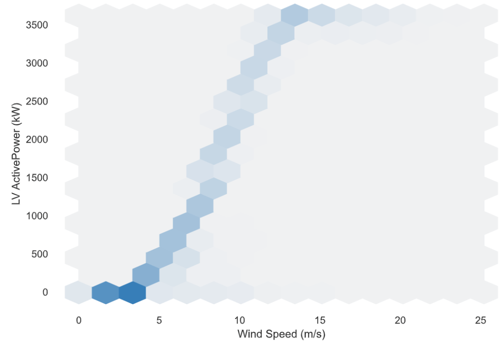
In wind turbines, the Scada system measures actual wind speed and direction vs LV Active Power (kW) for 10 minutes intervals.

In addition to the observed power curve, the theoretical power curve is provided by the turbine manufacturer.
In this study, the input public-domain T1 dataset was taken from the Scada system that is working and generating wind power in Turkey.

Let’s set the working directory YOURPATH

import os
os.chdir('YOURPATH')    # Set working directory
os. getcwd()

Let’s import the key libraries

import matplotlib
import matplotlib.pyplot as plt
import matplotlib.style as style
import numpy as np
import pandas as pd
import plotly.express as px
import seaborn as sns
from scipy import stats
import warnings
warnings.filterwarnings("ignore")

and read the T1 data

data = pd.read_csv('T1.csv')

Let’s examine the shape and descriptive statistics of this dataset

data.shape

Output: (50530, 5)

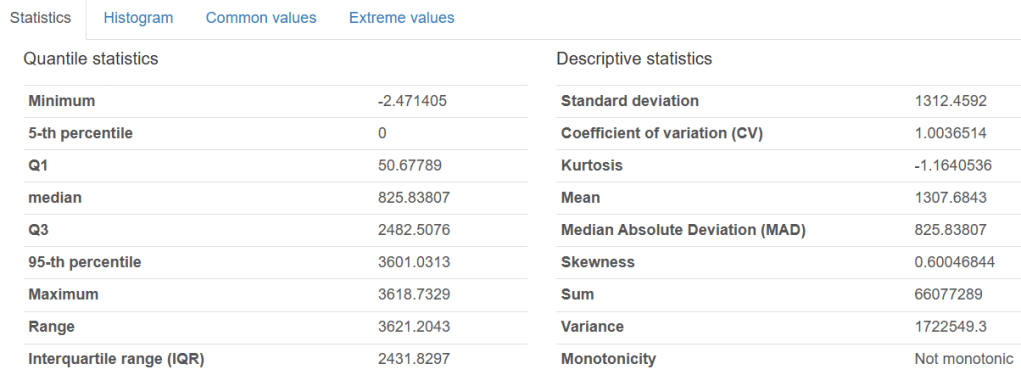
data.describe().T

Automated Exploratory Data Analysis (EDA)

Let’s generate the Pandas Profiling HTML report

import pandas as pd
from pandas_profiling import ProfileReport

profile = ProfileReport(data, title="Pandas Scada Data Report")
profile.to_file("reportscada.html")

Overview:

Variable types

Categorical	1
Numeric	4

Dataset statistics:

Number of variables	5
Number of observations	50530
Missing cells	0
Missing cells (%)	0.0%
Duplicate rows	0
Duplicate rows (%)	0.0%
Total size in memory	1.9 MiB
Average record size in memory	40.0 B

Alerts:

Variables:

LV ActivePower (kW)

Interactions:

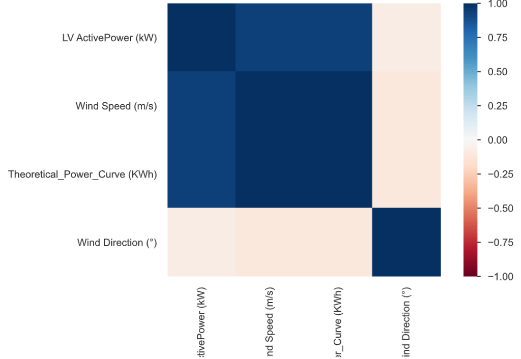
Correlations:

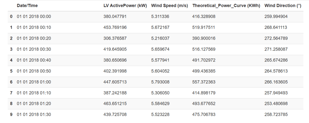
Sample

First rows

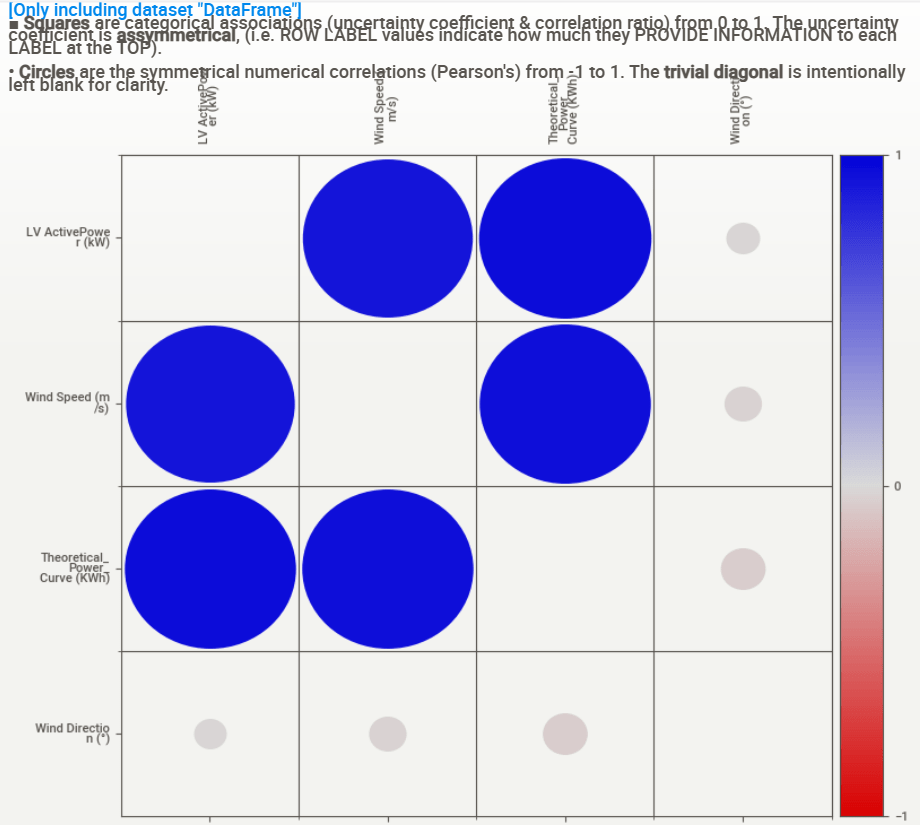
We can also generate the SweetViz report

# importing sweetviz
import sweetviz as sv
#analyzing the dataset
advert_report = sv.analyze(data)
#display the report
advert_report.show_html('scada_sweetviz.html')

Associations:

ML-Based Predictions of Wind Turbine Power Production

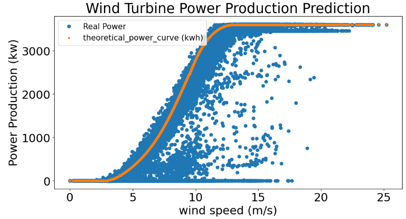
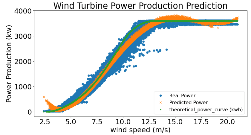
Let’s compare theoretical and observed power curves

matplotlib.rcParams.update({'font.size': 22})

data = data
exp = data['LV ActivePower (kW)']
the = data['Theoretical_Power_Curve (KWh)']
plt.figure(figsize=(12,6)) 
plt.plot(data['Wind Speed (m/s)'], data['LV ActivePower (kW)'], 'o', label='Real Power')
plt.plot(data['Wind Speed (m/s)'], data['Theoretical_Power_Curve (KWh)'], '.', label='theoretical_power_curve (kwh)')
plt.xlabel('wind speed (m/s)', size=22)
plt.ylabel('Power Production (kw)', size=22)
plt.title('Wind Turbine Power Production Prediction')
plt.legend(loc ="upper left",fontsize=15)
plt.show()

Let’s import ML libraries and perform data pre-processing:

from sklearn import metrics
from sklearn import model_selection
from sklearn import preprocessing
from sklearn.datasets import make_classification
from sklearn.ensemble import ExtraTreesRegressor
from sklearn.ensemble import GradientBoostingClassifier
from sklearn.ensemble import GradientBoostingRegressor
from sklearn.ensemble import RandomForestClassifier
from sklearn.ensemble import RandomForestRegressor
from sklearn.linear_model import ElasticNet
from sklearn.linear_model import Lasso
from sklearn.linear_model import LinearRegression
from sklearn.linear_model import LogisticRegression
from sklearn.linear_model import Ridge
from sklearn.metrics import accuracy_score
from sklearn.metrics import classification_report, confusion_matrix
from sklearn.metrics import mean_squared_error
from sklearn.metrics import mean_squared_error, mean_absolute_error

from sklearn.model_selection import cross_val_score
from sklearn.model_selection import train_test_split
from sklearn.naive_bayes import GaussianNB
from sklearn.neighbors import KNeighborsClassifier
from sklearn.neighbors import KNeighborsRegressor
from sklearn.preprocessing import StandardScaler, Normalizer
from sklearn.tree import DecisionTreeClassifier
from sklearn.tree import DecisionTreeRegressor
from xgboost import XGBClassifier
from xgboost.sklearn import XGBRegressor
import xgboost as xgb

def outlier_remover(dat, prop, min, max):
    d = dat
    q_low = d[prop].quantile(min)
    q_hi  = d[prop].quantile(max)
    return d[(d[prop] < q_hi) & (d[prop] > q_low)]

# Create Sub-DataFrames
d = {}
step = 50
i = 1
for x in range(20, 3400, step):
    d[i] = data.iloc[((data['LV ActivePower (kW)']>=x)&((data['LV ActivePower (kW)']<x+step))).values]
    #print(d[i])
    i = i + 1
print("There are in total of {} DataFrames".format(i-1))

Output: There are in total of 68 DataFrames

d[69] = data.iloc[(data['LV ActivePower (kW)']>=3300).values]

# Remove outlier
for x in range(1, 70):
    if x <= 3:
        F = 0.95
    elif ((x > 3) and (x <= 10)):
        F = 0.9
    elif ((x > 10) and (x <= 20)):
        F = 0.92
    elif ((x > 20) and (x < 30)):
        F = 0.96
    else:
        F = 0.985
    d[x] = outlier_remover(d[x], 'Wind Speed (m/s)', 0.0001, F)

df=pd.DataFrame()
for infile in range(1,70):
    data = d[infile]
    df=df.append(data,ignore_index=True)

df.shape

Output: (37803, 5)

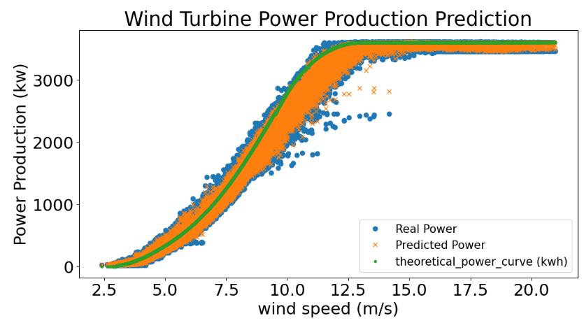
Let’s compare theoretical and observed power curves after editing of observed data

matplotlib.rcParams.update({'font.size': 22})

data = df
exp = data['LV ActivePower (kW)']
the = data['Theoretical_Power_Curve (KWh)']
plt.figure(figsize=(12,6)) 
plt.plot(data['Wind Speed (m/s)'], data['LV ActivePower (kW)'], 'o', label='Real Power')
plt.plot(data['Wind Speed (m/s)'], data['Theoretical_Power_Curve (KWh)'], '.', label='theoretical_power_curve (kwh)')
plt.xlabel('wind speed (m/s)', size=22)
plt.ylabel('Power Production (kw)', size=22)
plt.title('Wind Turbine Power Production Prediction')
plt.legend(fontsize=15,loc ="lower right")
plt.show()

Observed vs theoretical power curves after observed data editing

Let’s introduce the following functions needed for ML training

ftrain = ['LV ActivePower (kW)', 'Wind Speed (m/s)', 'Wind Direction (°)']

def Definedata():
    # define dataset
    data2 = df[ftrain]
    X = data2.drop(columns=['LV ActivePower (kW)']).values
    y = data2['LV ActivePower (kW)'].values
    return X, y

def Models(models):
    
    model = models
    X, y = Definedata()
    X_train, X_test, y_train, y_test = train_test_split(X, y, test_size = 0.2, random_state = 125)
    model.fit(X_train,y_train)
    y_pred = model.predict(X_test)
    y_total = model.predict(X)
    
    print("\t\tError Table")
    print('Mean Absolute Error      : ', metrics.mean_absolute_error(y_test, y_pred))
    print('Mean Squared  Error      : ', metrics.mean_squared_error(y_test, y_pred))
    print('Root Mean Squared  Error : ', np.sqrt(metrics.mean_squared_error(y_test, y_pred)))
    print('Accuracy on Training set   : ', model.score(X_train,y_train))
    print('Accuracy on Testing set  : ', model.score(X_test,y_test))
    return y_total, y

def Featureimportances(models):
    model = models
    model.fit(X_train,y_train)
    importances = model.feature_importances_
    features = df_test.columns[:9]
    imp = pd.DataFrame({'Features': ftest, 'Importance': importances})
    imp['Sum Importance'] = imp['Importance'].cumsum()
    imp = imp.sort_values(by = 'Importance')
    return imp

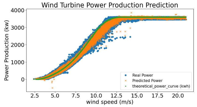
def Graph_prediction(y_actual, y_predicted):
    matplotlib.rcParams.update({'font.size': 22})
    y = y_actual
    y_total = y_predicted
    TP = df['Theoretical_Power_Curve (KWh)']
    number = len(df['Wind Speed (m/s)'])
    aa=[x for x in df['Wind Speed (m/s)']]
    plt.figure(figsize=(12,6)) 
    plt.plot(aa, y[:number], 'o', label='Real Power')
    plt.plot(aa, y_total[:number], 'x', label='Predicted Power')
    plt.plot(aa, TP[:number], '.', label='theoretical_power_curve (kwh)')
    
    plt.xlabel('wind speed (m/s)', size=22)
    plt.ylabel('Power Production (kw)', size=22)
    plt.title('Wind Turbine Power Production Prediction')
    plt.legend(fontsize=15,loc ="lower right")
    plt.show()

KNeighborsRegressor (KNN)

y_predicted, y_actual = Models(KNeighborsRegressor())
Graph_prediction(y_actual, y_predicted)

Error Table 

Mean Absolute Error : 84.9877243162573 

Mean Squared Error : 15990.241699106758 

Root Mean Squared Error : 126.45252745242682 

Accuracy on Training set : 0.9936902804656327 

Accuracy on Testing set : 0.9899973865944977

Power curve predicted by DecisionTreeRegressor() vs observed data and theoretical power curve

DecisionTreeRegressor (DT)

y_predicted, y_actual = Models(DecisionTreeRegressor())
Graph_prediction(y_actual, y_predicted)

Error Table 

Mean Absolute Error : 97.4102137065757 

Mean Squared Error : 22350.459953375295 

Root Mean Squared Error : 149.50070218355262 

Accuracy on Training set : 1.0 

Accuracy on Testing set : 0.9860187847966511

Power curve predicted by ExtraTreesRegressor() vs observed data and theoretical power curve

ExtraTreesRegressor (ET)

y_predicted, y_actual = Models(ExtraTreesRegressor())
Graph_prediction(y_actual, y_predicted)

Error Table 

Mean Absolute Error : 79.52242681022484 

Mean Squared Error : 14759.43257128833 

Root Mean Squared Error : 121.48840508990284 

Accuracy on Training set : 1.0 

Accuracy on Testing set : 0.9907673129103843

Power curve predicted by KNeighborsRegressor() vs observed data and theoretical power curve

RandomForestRegressor (RF)

y_predicted, y_actual = Models(RandomForestRegressor(n_estimators=350,min_samples_split=2,min_samples_leaf=1,max_features='sqrt',max_depth=25))
Graph_prediction(y_actual, y_predicted)

Error Table
Mean Absolute Error      :  76.44924832499083
Mean Squared  Error      :  12987.579768252423
Root Mean Squared  Error :  113.96306317510259
Accuracy on Training set   :  0.9988794773674271
Accuracy on Testing set  :  0.9918756863129712

Power curve predicted by RandomForestRegressor() vs observed data and theoretical power curve

GradientBoostingRegressor (GB)

y_predicted, y_actual = Models(GradientBoostingRegressor(random_state=21, n_estimators=2000))
Graph_prediction(y_actual, y_predicted)

Error Table
Mean Absolute Error      :  75.85085775100555
Mean Squared  Error      :  12444.035639985173
Root Mean Squared  Error :  111.55283788405015
Accuracy on Training set   :  0.9949454619292175
Accuracy on Testing set  :  0.9922156975452086

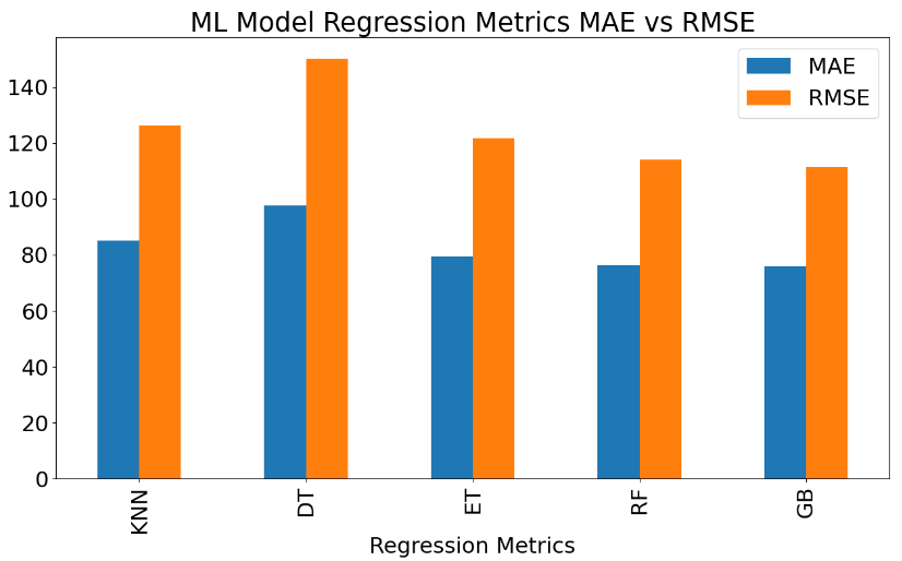
Power curve predicted by GradientBoostingRegressor() vs observed data and theoretical power curve

Let’s create the following ML performance summary bar chart

import pandas as pd

matplotlib.rcParams.update({'font.size': 22})



plotdata = pd.DataFrame({

    "MAE":[84.98,97.70,79.46,76.39,75.85],

    "RMSE":[126.45,150.26,121.75,113.96,111.55]},

    index=['KNN','DT',"ET", "RF", "GB"])

plotdata.plot(kind="bar",figsize=(15, 8))

plt.title("ML Model Regression Metrics MAE vs RMSE")

plt.xlabel("Regression Metrics",size=22)

plt.legend(fontsize=22,loc ="upper right")

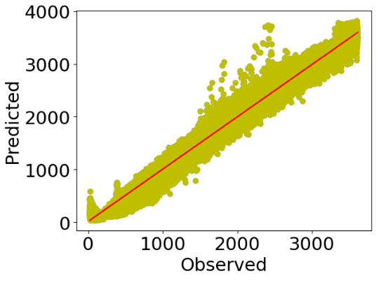
ML Model Regression Metrics MAE vs RMSE for 5 ML models

Polynomial Regression

Let’s test the polynomial regression algorithm

from sklearn.preprocessing import PolynomialFeatures
poly_regressor = PolynomialFeatures(degree=4)
X, y = Definedata()
X_columns = poly_regressor.fit_transform(X)
from sklearn.linear_model import LinearRegression
model = LinearRegression()

model.fit(X_columns, y)

pred = model.predict(poly_regressor.fit_transform(X))

Let’s look at the scatter X-plot

plt.scatter(y,pred)
xx=y
yy=pred
m, b = np.polyfit(xx, yy, 1)

plt.plot(xx, yy, 'yo', xx, m*xx+b, '--r')

matplotlib.rcParams.update({'font.size': 22})
plt.xlabel("Observed",size=22)
plt.ylabel("Predicted",size=22)

plt.show()

Predicted vs Observed data X-plot of the 4th order polynomial regression

The corresponding power curves are as follows

y = y
    y_total = pred
    TP = df['Theoretical_Power_Curve (KWh)']
    number = len(df['Wind Speed (m/s)'])
    aa=[x for x in df['Wind Speed (m/s)']]
    matplotlib.rcParams.update({'font.size': 22})
    plt.figure(figsize=(12,6)) 
    plt.plot(aa, y[:number], 'o', label='Real Power')
    plt.plot(aa, y_total[:number], 'x', label='Predicted Power')
    plt.plot(aa, TP[:number], '.', label='theoretical_power_curve (kwh)')
    
    plt.xlabel('wind speed (m/s)', size=22)
    plt.ylabel('Power Production (kw)', size=22)
    plt.title('Wind Turbine Power Production Prediction')
    plt.legend(fontsize=15)
    plt.show()

Power curve predicted by the 4th order polynomial regression vs observed data and theoretical power curve

Wind Turbine Power Curve Simulations and Control

Let’s turn our attention to the T1 power curve control:

Import libraries

import numpy as np 
import pandas as pd 
import seaborn as sns
import matplotlib.pyplot as plt
from collections import Counter
%matplotlib inline
import openpyxl
import chart_studio.plotly
from plotly.offline import init_notebook_mode, iplot
init_notebook_mode(connected=True)
import plotly.graph_objs as go

Data preparation

def find_month(x):
    if " 01 " in x:
        return "Jan"
    elif " 02 " in x:
        return "Feb"
    elif " 03 " in x:
        return "March"    
    elif " 04 " in x:
        return "April"    
    elif " 05 " in x:
        return "May"    
    elif " 06 " in x:
        return "June"    
    elif " 07 " in x:
        return "July"    
    elif " 08 " in x:
        return "August"    
    elif " 09 " in x:
        return "Sep"    
    elif " 10 " in x:
        return "Oct"    
    elif " 11 " in x:
        return "Nov"    
    else:
        return "Dec"

def mean_speed(x):
    list=[]
    i=0.25
    while i<=25.5:
        list.append(i)
        i+=0.5
        
    for i in list:
        if x < i:
            x=i-0.25
            return x

def mean_direction(x):
    list=[]
    i=15
    while i<=375:
        list.append(i)
        i+=30
        
    for i in list:
        if x < i:
            x=i-15
            if x==360:
                return 0
            else:
                return x

def find_direction(x):
    if x==0:
        return "N"
    if x==30:
        return "NNE"
    if x==60:
        return "NEE" 
    if x==90:
        return "E" 
    if x==120:
        return "SEE" 
    if x==150:
        return "SSE" 
    if x==180:
        return "S" 
    if x==210:
        return "SSW" 
    if x==240:
        return "SWW" 
    if x==270:
        return "W" 
    if x==300:
        return "NWW" 
    if x==330:
        return "NNW"

data_T_start=pd.read_csv("T1.csv")
turbine_no="T1" 
data1_T=data_T_start.copy()
data1_T["Month"]=data1_T["LV ActivePower (kW)"]+data1_T["Wind Speed (m/s)"]
data1_T.rename(columns={'LV ActivePower (kW)':'ActivePower(kW)',"Wind Speed (m/s)":"WindSpeed(m/s)","Wind Direction (°)":"Wind_Direction"},
                inplace=True)
data1_T.rename(columns={'Date/Time':'Time'},inplace=True)
data1_T.Month=data1_T.Time.apply(find_month)
data1_T["mean_WindSpeed"]=data1_T["WindSpeed(m/s)"].apply(mean_speed)
data1_T["mean_Direction"]=data1_T["Wind_Direction"].apply(mean_direction)
data1_T["Direction"]=data1_T["mean_Direction"].apply(find_direction)

Data cleaning

Remove the data that wind speed is <3.5 and >25.5.

Eliminate data where wind speed is >3.5 and active power =0.

data2_T=data1_T[(data1_T["WindSpeed(m/s)"]>3.5) & (data1_T["WindSpeed(m/s)"]<=25.5)]
data3_T=data2_T[((data2_T["ActivePower(kW)"]!=0)&(data2_T["WindSpeed(m/s)"]>3.5)) | (data2_T["WindSpeed(m/s)"]<=3.5)]

Calculate the mean value of Powercurve(kW) when mean_WindSpeed is 5.5

data3_T["Theoretical_Power_Curve (KWh)"][data3_T["mean_WindSpeed"]==5.5].mean()

Output: 472.09575192642797

Loss Calculations

data_T_clean=data3_T.sort_values("Time")
data_T_clean["Loss_Value(kW)"]=data_T_clean["Theoretical_Power_Curve (KWh)"]-data_T_clean["ActivePower(kW)"]
data_T_clean["Loss(%)"]=data_T_clean["Loss_Value(kW)"]/data_T_clean["Theoretical_Power_Curve (KWh)"]*100
#round the values to 2 digit
data_T_clean=data_T_clean.round({'ActivePower(kW)': 2, 'WindSpeed(m/s)': 2, 'Theoretical_Power_Curve (KWh)': 2,
                                   'Wind_Direction': 2, 'Loss_Value(kW)': 2, 'Loss(%)': 2})

Create the final summary DataFrame

DepGroupT_speed = data_T_clean.groupby("mean_WindSpeed")
data_T_speed=DepGroupT_speed.mean()
#remove the unnecessary columns.
data_T_speed.drop(columns={"WindSpeed(m/s)","Wind_Direction","mean_Direction"},inplace=True)
#create a windspeed column from index values.
listTspeed_WS=data_T_speed.index.copy()
data_T_speed["WindSpeed(m/s)"]=listTspeed_WS
#change the place of columns.
data_T_speed=data_T_speed[["WindSpeed(m/s)","ActivePower(kW)","Theoretical_Power_Curve (KWh)","Loss_Value(kW)","Loss(%)"]]
#change the index numbers.
data_T_speed["Index"]=list(range(1,len(data_T_speed.index)+1))
data_T_speed.set_index("Index",inplace=True)
#del data_T_speed.index.name
#round the values to 2 digit
data_T_speed=data_T_speed.round({"WindSpeed(m/s)": 1, 'ActivePower(kW)': 2, 'Theoretical_Power_Curve (KWh)': 2, 'Loss_Value(kW)': 2, 'Loss(%)': 2})
#create a count column that shows the number of wind speed from clean data.
data_T_speed["count"]=[len(data_T_clean["mean_WindSpeed"][data_T_clean["mean_WindSpeed"]==i]) 
                        for i in data_T_speed["WindSpeed(m/s)"]]
DepGroupT_direction = data_T_clean.groupby("Direction")
data_T_direction=DepGroupT_direction.mean()
#remove the unnecessary columns.
data_T_direction.drop(columns={"WindSpeed(m/s)","Wind_Direction"},inplace=True)
#create a column from index.
listTdirection_Dir=data_T_direction.index.copy()
data_T_direction["Direction"]=listTdirection_Dir
#change the name of mean_WindSpeed column as  WindSpeed.
data_T_direction["WindSpeed(m/s)"]=data_T_direction["mean_WindSpeed"]
data_T_direction.drop(columns={"mean_WindSpeed"},inplace=True)
#change the place of columns.
data_T_direction=data_T_direction[["Direction","mean_Direction","ActivePower(kW)","Theoretical_Power_Curve (KWh)","WindSpeed(m/s)",
                                     "Loss_Value(kW)","Loss(%)"]]
#change the index numbers.
data_T_direction["Index"]=list(range(1,len(data_T_direction.index)+1))
data_T_direction.set_index("Index",inplace=True)
#del data_T_direction.index.name
#create a count column that shows the number of directions from clean data.
data_T_direction["count"]=[len(data_T_clean["Direction"][data_T_clean["Direction"]==i]) 
                        for i in data_T_direction["Direction"]]
#round the values to 2 digit
data_T_direction=data_T_direction.round({'WindSpeed(m/s)': 1,'ActivePower(kW)': 2, 'Theoretical_Power_Curve (KWh)': 2,
                                           'Loss_Value(kW)': 2, 'Loss(%)': 2})
#sort by mean_Direction
data_T_direction=data_T_direction.sort_values("mean_Direction")
data_T_direction.drop(columns={"mean_Direction"},inplace=True)

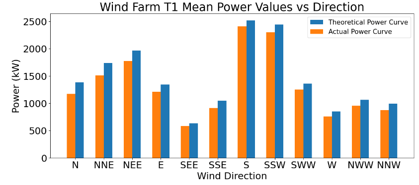
Mean Power vs Direction

#Drawing graph of mean powers according to wind direction.
def bar_graph():
    fig = plt.figure(figsize=(15,6))
    matplotlib.rcParams.update({'font.size': 22})
    plt.bar(data_T_direction["Direction"],data_T_direction["Theoretical_Power_Curve (KWh)"],label="Theoretical Power Curve",align="edge",width=0.3)
    plt.bar(data_T_direction["Direction"],data_T_direction["ActivePower(kW)"],label="Actual Power Curve",align="edge",width=-0.3)
    plt.xlabel("Wind Direction",size=22)
    plt.ylabel("Power (kW)",size=22)
    plt.title("Wind Farm {} Mean Power Values vs Direction".format(turbine_no))
    plt.legend(fontsize=15)
    plt.show()
bar_graph()

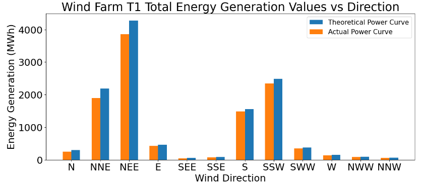
Total energy generation vs direction

#create summary direction total dataframe from direction data.
data_T_direction_total=data_T_direction.copy()
#remove the unnecessary columns.
data_T_direction_total.drop(columns={"count","ActivePower(kW)","Theoretical_Power_Curve (KWh)","Loss_Value(kW)","Loss(%)"},inplace=True)
#calculate the total values from direction data.
data_T_direction_total["Total_Generation(MWh)"]=data_T_direction["ActivePower(kW)"]*data_T_direction["count"]/6000
data_T_direction_total["Theoretical_PC_Total_Generation(MWh)"]=data_T_direction["Theoretical_Power_Curve (KWh)"]*data_T_direction["count"]/6000
data_T_direction_total["Total_Loss(MWh)"]=data_T_direction_total["Theoretical_PC_Total_Generation(MWh)"]-data_T_direction_total["Total_Generation(MWh)"]
data_T_direction_total["Loss(%)"]=data_T_direction_total["Total_Loss(MWh)"]/data_T_direction_total["Theoretical_PC_Total_Generation(MWh)"]*100
#round the values to 2 digit
data_T_direction_total=data_T_direction_total.round({'WindSpeed(m/s)': 1,'Total_Generation(MWh)': 2, 'Theoretical_PC_Total_Generation(MWh)': 2,
                                           'Total_Loss(MWh)': 2, 'Loss(%)': 2})
#change the place of columns.
data_T_direction_total=data_T_direction_total[["Direction","Total_Generation(MWh)","Theoretical_PC_Total_Generation(MWh)","WindSpeed(m/s)",
                                     "Total_Loss(MWh)","Loss(%)"]]

#Drawing graph of total generations according to wind direction.
def bar_graph():
    fig = plt.figure(figsize=(15,6))
    matplotlib.rcParams.update({'font.size': 22})
    plt.bar(data_T_direction_total["Direction"],data_T_direction_total["Theoretical_PC_Total_Generation(MWh)"],label="Theoretical Power Curve",align="edge",width=0.3)
    plt.bar(data_T_direction_total["Direction"],data_T_direction_total["Total_Generation(MWh)"],label="Actual Power Curve",align="edge",width=-0.3)
    plt.xlabel("Wind Direction",size=22)
    plt.ylabel("Energy Generation (MWh)",size=22)
    plt.title("Wind Farm {} Total Energy Generation Values vs Direction".format(turbine_no))
    plt.legend(fontsize=15)
    plt.show()
bar_graph()

Total energy loss vs direction

ef bar_graph():
    fig = plt.figure(figsize=(15,6))
    matplotlib.rcParams.update({'font.size': 22})
    plt.bar(data_T_direction_total["Direction"],data_T_direction_total["Total_Loss(MWh)"],
            label="Total_Loss(MWh)",align="center",width=0.5, color="red",picker=5)
    plt.xlabel("Wind Direction",size=22)
    plt.ylabel("Total Loss (MWh)",size=22)
    plt.title("Wind Farm {} Total Loss Values vs Direction".format(turbine_no))
    plt.legend(fontsize=15)
    plt.show()
bar_graph()

Create the summary DataFrame for all directions

list_data=[]
list_yon=["N","NNE","NEE","E","SEE","SSE","S","SSW","SWW","W","NWW","NNW"]
for i in range(0,12):
    data1T_A=data_T_clean[data_T_clean["Direction"]==list_yon[i]]
    #
    DepGroup_A = data1T_A.groupby("mean_WindSpeed")
    data_T_A=DepGroup_A.mean()
    #
    data_T_A.drop(columns={"WindSpeed(m/s)","Wind_Direction","mean_Direction"},inplace=True)
    #
    listTA_WS=data_T_A.index.copy()
    data_T_A["WindSpeed(m/s)"]=listTA_WS
    #
    data_T_A=data_T_A[["WindSpeed(m/s)","ActivePower(kW)","Theoretical_Power_Curve (KWh)","Loss_Value(kW)","Loss(%)"]]
    #
    data_T_A["Index"]=list(range(1,len(data_T_A.index)+1))
    data_T_A.set_index("Index",inplace=True)
#    del data_T_A.index.name
    #
    data_T_A=data_T_A.round({'ActivePower(kW)': 2, 'Theoretical_Power_Curve (KWh)': 2, 'Loss_Value(kW)': 2, 'Loss(%)': 2})
    #
    data_T_A["count"]=[len(data1T_A["mean_WindSpeed"][data1T_A["mean_WindSpeed"]==x]) 
                            for x in data_T_A["WindSpeed(m/s)"]]
    list_data.append(data_T_A)
    
data_T_N=list_data[0]
data_T_NNE=list_data[1]
data_T_NEE=list_data[2]
data_T_E=list_data[3]
data_T_SEE=list_data[4]
data_T_SSE=list_data[5]
data_T_S=list_data[6]
data_T_SSW=list_data[7]
data_T_SWW=list_data[8]
data_T_W=list_data[9]
data_T_NWW=list_data[10]
data_T_NNW=list_data[11]

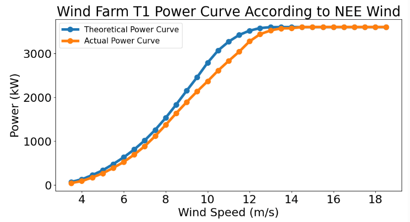
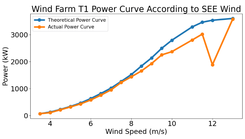
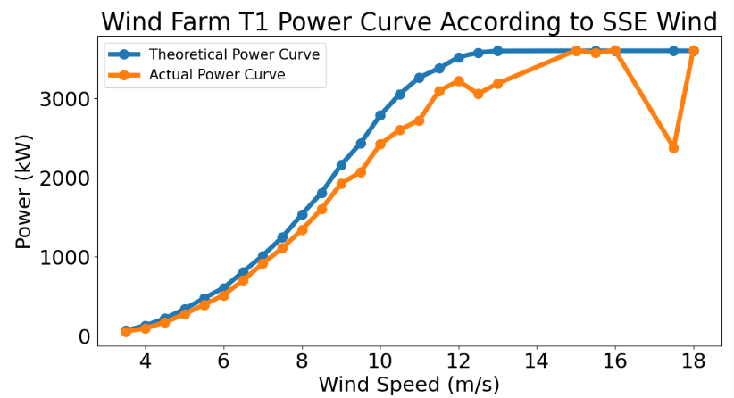
Plotting the T1 power curve for all directions

def graph_WT():
    fig = plt.figure(figsize=(12,6))
    matplotlib.rcParams.update({'font.size': 22})
    plt.plot(data_T_speed["WindSpeed(m/s)"],data_T_speed["Theoretical_Power_Curve (KWh)"],label="Theoretical Power Curve",
             marker="o",markersize=10,linewidth = 5)
    plt.plot(data_T_speed["WindSpeed(m/s)"],data_T_speed["ActivePower(kW)"],label="Actual Power Curve",
             marker="o",markersize=10,linewidth = 5)
    plt.xlabel("Wind Speed (m/s)",size=22)
    plt.ylabel("Power (kW)",size=22)
    plt.title("Wind Farm {} Power Curve".format(turbine_no))
    plt.legend()
    plt.show()
graph_WT()

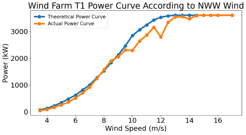
Plotting the T1 power curve vs direction bin

list_table=[data_T_N,data_T_NNE,data_T_NEE,data_T_E,data_T_SEE,data_T_SSE,data_T_S,
            data_T_SSW,data_T_SWW,data_T_W,data_T_NWW,data_T_NNW]

list_tableName=["N","NNE","NEE","E","SEE","SSE","S","SSW","SWW","W","NWW","NNW"]

def graph_T(i):
    fig = plt.figure(figsize=(12,6))  
    matplotlib.rcParams.update({'font.size': 22})
    plt.plot(list_table[i]["WindSpeed(m/s)"],list_table[i]["Theoretical_Power_Curve (KWh)"],label="Theoretical Power Curve",
             marker="o",markersize=10,linewidth = 5)
    plt.plot(list_table[i]["WindSpeed(m/s)"],list_table[i]["ActivePower(kW)"],label="Actual Power Curve",
             marker="o",markersize=10,linewidth = 5)
    plt.xlabel("Wind Speed (m/s)",size=22)
    plt.ylabel("Power (kW)",size=22)
    plt.title("Wind Farm {} Power Curve According to {} Wind".format(turbine_no,list_tableName[i]))
    plt.legend(fontsize=15)
    plt.show()
for i in range(0,12):
    graph_T(i)

Summary

A wind turbine is characterized by a power curve representing the relation between the wind speed and the amount of generated electrical power.
We have conducted this study to find the best performing regression algorithm to model power curves.
We have tested and validated our models using real Scada data from a wind farm.
The study showed that very accurate power curves can be created based upon supervised ML techniques such as Random Forest and Gradient Boosting Regressors.
Using observed winds and power production at an operational site, we have shown that both wind speed and direction affect the average energy generation and loss.
The final Python workflow is straightforward to implement and does not rely on assumptions about the wind or stability.
Industry applications include wind turbine selection, capacity factor estimation, wind energy assessment and forecasting, and condition monitoring.

Explore More

Go back

Your message has been sent

Make a one-time donation

Make a monthly donation

Make a yearly donation

Choose an amount

€5.00

€15.00

€100.00

€5.00

€15.00

€100.00

€5.00

€15.00

€100.00

Or enter a custom amount

€

Your contribution is appreciated.

Donate Donate monthly Donate yearly

Wind Energy ML Prediction & Turbine Power Control

The Wind Turbine Scada Dataset

Automated Exploratory Data Analysis (EDA)

ML-Based Predictions of Wind Turbine Power Production

Wind Turbine Power Curve Simulations and Control

Summary

Explore More

Your message has been sent

Make a one-time donation

Make a monthly donation

Make a yearly donation

Discover more from Our Blogs

Leave a comment Cancel reply

Wind Energy ML Prediction & Turbine Power Control

The Wind Turbine Scada Dataset

Automated Exploratory Data Analysis (EDA)

ML-Based Predictions of Wind Turbine Power Production

Wind Turbine Power Curve Simulations and Control

Summary

Explore More

Your message has been sent

Make a one-time donation

Make a monthly donation

Make a yearly donation

Share this:

Discover more from Our Blogs

Leave a comment Cancel reply

Discover more from Our Blogs