WA House Price Prediction: EDA-ML-HPO

Photo by Ian Keefe on Unsplash

• The objective of this post is to train and test an optimized multiple-ML model to predict sale price for houses in King County, WA. King county is the most populous county in WA, and the 12th most populous county in the United States.
• Inspired by the earlier studies, we use the GridSearchCV Cross Validation for choosing the best parameters of the following 5 top performing supervised ML regression models: LinearRegression (LR), SGDRegressor (SGD), RandomForestRegressor (RF), XGBRegressor (XGB), and AdaBoostRegressor (Ada).
• The important step in our study is the use of Automated EDA (Exploratory Data Analysis) packages that can perform EDA in a few lines of Python code. Specifically, we will utilize Pandas-Profiling and SweetViz to discover patterns, identify anomalies, and find relationships between variables.

Table of Contents

1. Input Dataset
2. Automated EDA
3. Data Preparation
4. House Price Map
5. Multiple-ML HPO
6. Final Comparison
7. Conclusions
8. Explore More

Input Dataset

The dataset set used for this analysis is the King County Houses Sales dataset prepared by the county assessor. The dataset contains 21,597 home features and sale price collected during the years 2014–2015. The final model included homes ranging in price from $78,000–$3,100,000.

Following is a description of the model features:

• price — Sale price (prediction target)
• bedrooms — Number of bedrooms
• bathrooms — Number of bathrooms
• sqft_living — Square footage of living space in the home
• sqft_lot — Square footage of the lot
• floors — Number of floors (levels) in house
• waterfront — Whether the house is on a waterfront
• view — Quality of view from house
• condition — How good the overall condition of the house is. Related to maintenance of house.
• grade — Overall grade of the house. Related to the construction and design of the house.
• sqft_above — Square footage of house apart from basement
• sqft_basement — Square footage of the basement
• zipcode — ZIP Code used by the United States Postal Service

Let’s set the working directory HOUSEPRICES

import os
os.chdir(‘HOUSEPRICES’)
os. getcwd()

and import the libraries

import os
import folium
import warnings
import numpy as np
import pandas as pd
import matplotlib.pyplot as plt
import seaborn as sns
from folium.plugins import HeatMap
folds = 5
sns.set(color_codes=True)
from sklearn.metrics import r2_score
from scipy import stats
from sklearn.model_selection import GridSearchCV
score_calc = ‘neg_mean_squared_error’

Let’s read the input data

house_data = pd.read_csv(‘kc_house_data.csv’)

Automated EDA

Let’s import the Pandas-Profiling library to be used for EDA and visualization

from pandas_profiling import ProfileReport
profile = ProfileReport(house_data, title=”Pandas Profiling Report”)
profile.to_file(“reportpandas.html”)

It creates the interactive HTML report reportpandas.html that displays various summary statistics and visualizations of house_data:

Overview

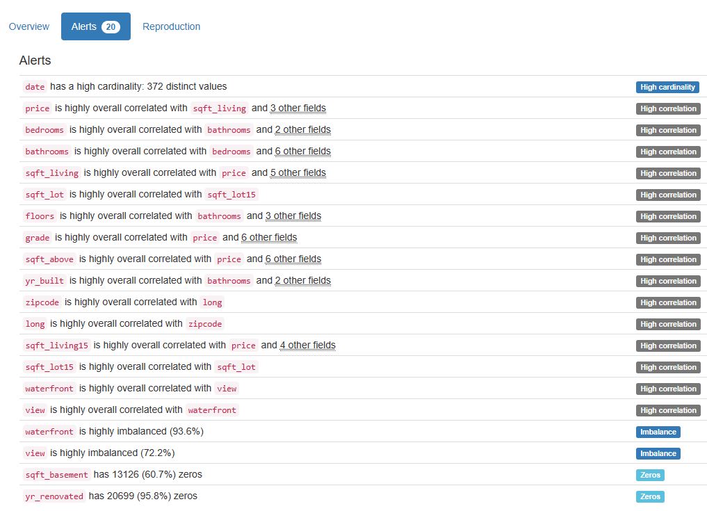
Variables

Interactions

Correlations

Let’s create an analysis report using sweetviz

import sweetviz as sv

eport = sv.analyze(house_data)

Let’s display the report
report.show_html()

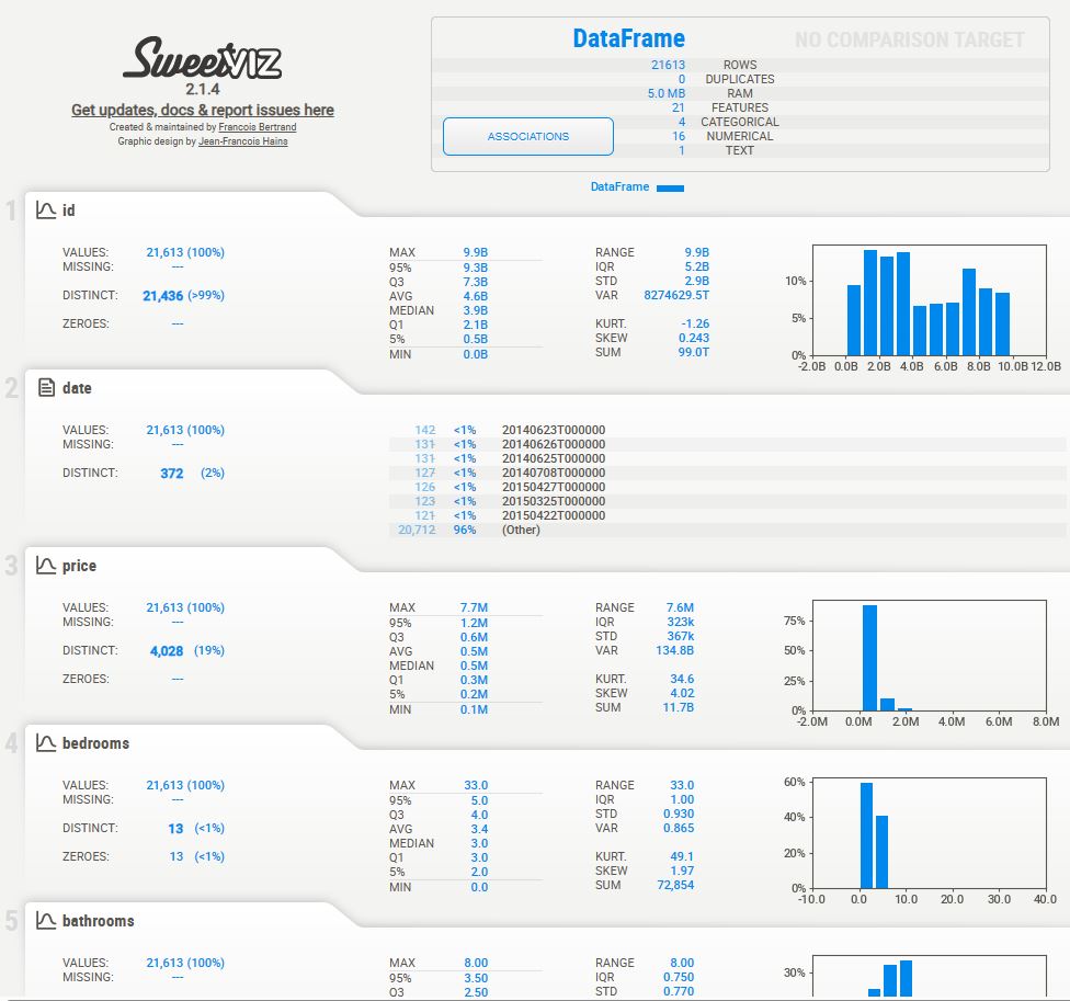
Associations

 Squares are categorical associations (uncertainty coefficient & correlation ratio) from 0 to 1. The uncertainty coefficient is assymmetrical, (i.e. ROW LABEL values indicate how much they PROVIDE INFORMATION to each LABEL at the TOP).

• Circles are the symmetrical numerical correlations (Pearson’s) from -1 to 1. The trivial diagonal is intentionally left blank for clarity.

Data Preparation

Let’s drop a few unnecessary columns

house_data_2 = house_data.drop([‘id’, ‘date’],axis=1)

Adding new features
house_data_2[“Home_Age”] = 2023 – house_data_2[“yr_built”]
house_data_2[‘is_renovated’] = house_data_2[“yr_renovated”].where(house_data_2[“yr_renovated”] == 0, 1)
house_data_2[‘Total_Area’] = house_data_2[‘sqft_living’] + house_data_2[‘sqft_lot’] + house_data_2[‘sqft_above’] + house_data_2[‘sqft_basement’]
house_data_2[‘Basement’] = house_data_2[‘sqft_basement’].where(house_data_2[“sqft_basement”] == 0, 1)

and dropping duplicates

house_data_3 = house_data_2.drop_duplicates()

Let’s calculate the ratios

house_data_3[“price_per_sqft_living”] = house_data_3[“price”]/house_data_3[“sqft_living”]
house_data_3[“price_per_total_area”] = house_data_3[“price”]/house_data_3[“Total_Area”]

and apply the following data thresholds

house_data_3[house_data_3[‘price_per_total_area’]>100]

house_data_4 = house_data_3[house_data_3[‘price_per_total_area’] <= 100]

house_data_5 = house_data_4[house_data_4[‘price_per_total_area’] > 5]

house_data_6 = house_data_5[house_data_5[‘price_per_sqft_living’]<=500]

house_data_7 = house_data_6[house_data_6[‘bedrooms’] < 7]

Let’s calculate the following ratios

house_data_7[‘price_per_floor’] = house_data_7[‘price’]/house_data_7[‘floors’]
house_data_7[‘price_per_view’] = house_data_7[‘price’]/house_data_7[‘view’]

Dropping features with poor correlation to price
house_data_8 = house_data_7.drop([‘price_per_view’, ‘sqft_lot15’, ‘long’,
‘waterfront’, ‘condition’, ‘zipcode’,
‘yr_renovated’, ‘is_renovated’, ‘Basement’,
‘Home_Age’, ‘yr_built’, ‘sqft_living15’],axis=1)

house_data_9 = house_data_8.drop([‘bathrooms’, ‘sqft_basement’,
‘lat’, ‘bedrooms’, ‘Total_Area’,
‘floors’, ‘view’], axis=1)

and dropping duplicates

house_data_10 = house_data_9.drop_duplicates()
house_data_10.duplicated().sum()

0

Let’s check the descriptive statistics of the target column ‘price’

house_data_10[‘price’].describe()

count 1.904900e+04

mean 4.969407e+05

std 2.739362e+05

min 8.000000e+04

25% 3.100000e+05

50% 4.310000e+05

75% 6.100000e+05

max 3.300000e+06

Name: price, dtype: float64

House Price Map

Visualizing the house price map

maxpr=house_data_7.loc[house_data_7[‘price’].idxmax()]

def generateBaseMap(default_location=[47.5112, -122.257], default_zoom_start=9.4):
base_map = folium.Map(location=default_location, control_scale=True, zoom_start=default_zoom_start)
return base_map

house_data_7_copy = house_data_7.copy()
house_data_7_copy[‘count’] = 1
basemap = generateBaseMap()
folium.TileLayer(‘cartodbpositron’).add_to(basemap)
s=folium.FeatureGroup(name=’icon’).add_to(basemap)
folium.Marker([maxpr[‘lat’], maxpr[‘long’]],popup=’Highest Price: $’+str(format(maxpr[‘price’],’.0f’)),
icon=folium.Icon(color=’green’)).add_to(s)

HeatMap(data=house_data_7_copy[[‘lat’,’long’,’count’]].groupby([‘lat’,’long’]).sum().reset_index().values.tolist(),
radius=8,max_zoom=13,name=’Heat Map’).add_to(basemap)
folium.LayerControl(collapsed=False).add_to(basemap)
basemap

No surprise that the top home prices are all clustered around downtown Seattle.

Multiple-ML HPO

Let’s train and test several ML model with HPO using the dataset house_data_10

from sklearn.preprocessing import StandardScaler
from sklearn.preprocessing import RobustScaler
from sklearn.preprocessing import MinMaxScaler
from sklearn.model_selection import train_test_split

target = house_data_10[“price”]
features = house_data_10.drop(“price”, axis = 1)

X_train, X_test, Y_train, Y_test = train_test_split(features, target,
test_size = 0.2,
random_state = 1)

sc = StandardScaler()
X_train_sc = pd.DataFrame(sc.fit_transform(X_train))
X_test_sc = pd.DataFrame(sc.transform(X_test))

def get_best_score(grid):

best_score = np.sqrt(-grid.best_score_)
print(best_score)    
print(grid.best_params_)
print(grid.best_estimator_)

return best_score

Linear Regression (LR)

from sklearn.linear_model import LinearRegression

LR GridSearchCV

linreg = LinearRegression()
parameters = {‘fit_intercept’:[True,False], ‘positive’:[True,False], ‘copy_X’:[True, False]}
grid_linear = GridSearchCV(linreg, parameters, cv = folds, verbose = 1 , scoring = score_calc)
grid_linear.fit(X_train_sc, Y_train)

sc_linear = get_best_score(grid_linear)

Fitting 5 folds for each of 8 candidates, totalling 40 fits 66518.01517233807 {‘copy_X’: True, ‘fit_intercept’: True, ‘positive’: True} LinearRegression(positive=True)

LR Fit & Predict

LR = LinearRegression()
LR.fit(X_train_sc, Y_train)
pred_linreg_all = LR.predict(X_train_sc)

LR RMSE & R2-Score

from sklearn.metrics import mean_squared_error, r2_score
lr_mse = mean_squared_error(Y_train, pred_linreg_all)
lr_rmse = np.sqrt(lr_mse)
lr_rmse

66418.20377364717

r2_score(Y_train, pred_linreg_all)

0.9411316842046102

SGDRegressor (SGD)

from sklearn.linear_model import SGDRegressor

SGD GridSearchCV

sgd = SGDRegressor()
parameters = {‘max_iter’ :[10000], ‘alpha’:[1e-05], ‘epsilon’:[1e-02], ‘fit_intercept’ : [True] }
grid_sgd = GridSearchCV(sgd, parameters, cv = folds, verbose = 0, scoring = score_calc)
grid_sgd.fit(X_train_sc, Y_train)

sc_sgd = get_best_score(grid_sgd)
pred_sgd = grid_sgd.predict(X_train_sc)

66651.64885381745

{‘alpha’: 1e-05, ‘epsilon’: 0.01, ‘fit_intercept’: True, ‘max_iter’: 10000} SGDRegressor(alpha=1e-05, epsilon=0.01, max_iter=10000)

SGD Train & Predict

sd = SGDRegressor()
sd.fit(X_train_sc, Y_train)
sd_pred = sd.predict(X_train_sc)

SGD Train RMSE & R2-Score

sd_mse = mean_squared_error(Y_train, sd_pred)
sd_rmse = np.sqrt(sd_mse)
sd_rmse

66544.53443852205

r2_score(Y_train, sd_pred)

0.9409075304124359

SGD Test Predict, RMSE & R2-Score

SD_pred = sd.predict(X_test_sc)

SD_mse = mean_squared_error(Y_test, SD_pred)
SD_rmse = np.sqrt(SD_mse)
SD_rmse

68330.26415796539

r2_score(Y_test, SD_pred)

0.9381019885268382

RandomForestRegressor (RF)

from sklearn.ensemble import RandomForestRegressor

RF GridSearchCV

param_grid = {‘min_samples_split’ : [3,4,6,10], ‘n_estimators’ : [70,100], ‘random_state’: [5] }
grid_rf = GridSearchCV(RandomForestRegressor(), param_grid, cv = folds, refit=True, verbose = 0, scoring = score_calc)
grid_rf.fit(X_train, Y_train)

sc_rf = get_best_score(grid_rf)
pred_rf = grid_rf.predict(X_train)

25641.23777655788

{‘min_samples_split’: 3, ‘n_estimators’: 100, ‘random_state’: 5} RandomForestRegressor(min_samples_split=3, random_state=5)

RF Fit & Predict

rf_reg = RandomForestRegressor()
rf_reg.fit(X_train_sc, Y_train)
rf_pred = rf_reg.predict(X_train_sc)

RF Train RMSE & R2-Score

rf_mse = mean_squared_error(Y_train, rf_pred)
rf_rmse = np.sqrt(rf_mse)
rf_rmse

9825.936010452602

r2_score(Y_train, rf_pred)

0.9987115866341476

RF Test RMSE & R2-Score

rfr_pred = rf_reg.predict(X_test_sc)

rfr_mse = mean_squared_error(Y_test, rfr_pred)
rfr_rmse = np.sqrt(rfr_mse)
rfr_rmse

25603.03613090776

r2_score(Y_test, rfr_pred)

0.9913097266751898

XGBRegressor (XGB)

from xgboost import XGBRegressor

XGB GridSearchCV Train Fit, Predict & RMSE
param_grid = {‘learning_rate’ : [0.005,0.01,0.001], ‘n_estimators’ : [40,200], ‘random_state’: [5],
‘max_depth’ : [4,9]}
grid_xgb = GridSearchCV(XGBRegressor(), param_grid, cv = folds, refit=True, verbose = 0, scoring = score_calc)
grid_xgb.fit(X_train, Y_train)

sc_xgb = get_best_score(grid_xgb)
pred_xgb = grid_xgb.predict(X_train)

83083.50687697844

{‘learning_rate’: 0.01, ‘max_depth’: 9, ‘n_estimators’: 200, ‘random_state’: 5} XGBRegressor(base_score=0.5, booster=’gbtree’, callbacks=None, colsample_bylevel=1, colsample_bynode=1, colsample_bytree=1, early_stopping_rounds=None, enable_categorical=False, eval_metric=None, feature_types=None, gamma=0, gpu_id=-1, grow_policy=’depthwise’, importance_type=None, interaction_constraints=”, learning_rate=0.01, max_bin=256, max_cat_threshold=64, max_cat_to_onehot=4, max_delta_step=0, max_depth=9, max_leaves=0, min_child_weight=1, missing=nan, monotone_constraints='()’, n_estimators=200, n_jobs=0, num_parallel_tree=1, predictor=’auto’, random_state=5, …)

Normal XGB Train Fit, Predict & RMSE

xgb = XGBRegressor()
xgb.fit(X_train_sc, Y_train)
xgb_pred = xgb.predict(X_train_sc)
xgb_mse = mean_squared_error(Y_train, xgb_pred)
xgb_rmse = np.sqrt(xgb_mse)
xgb_rmse

8616.954073373103

XGB Test Predict, RMSE & R2-Score: Normal vs GridSearchCV

XGB_pred = xgb.predict(X_test_sc)
XGB_mse = mean_squared_error(Y_test, XGB_pred)
XGB_rmse = np.sqrt(XGB_mse)
XGB_rmse

18472.681261373717

pred_xgb = grid_xgb.predict(X_test)
Xgb_mse = mean_squared_error(Y_test, pred_xgb)
Xgb_rmse = np.sqrt(Xgb_mse)
Xgb_rmse

83969.73243389862

r2_score(Y_test, pred_xgb), r2_score(Y_test, XGB_pred)

(0.9065248788968281, 0.9954761273444909)

AdaBoostRegressor (Ada)

from sklearn.ensemble import AdaBoostRegressor
Ada Train Fit, Predict, RMSE & R2-Score

ada_reg = AdaBoostRegressor(DecisionTreeRegressor(),learning_rate=0.1, random_state=42)
ada_reg.fit(X_train_sc, Y_train)

AdaBoostRegressor(estimator=DecisionTreeRegressor(), learning_rate=0.1, random_state=42)

ada_pred = ada_reg.predict(X_train_sc)
ada_mse = mean_squared_error(Y_train, ada_pred)
ada_rmse = np.sqrt(ada_mse)
ada_rmse

7.561316168386757

r2_score(Y_train, ada_pred)

0.9999999992370393

Ada Test Predict, RMSE & R2-Score

Ada_pred = ada_reg.predict(X_test_sc)
Ada_mse = mean_squared_error(Y_test, Ada_pred)
Ada_rmse = np.sqrt(Ada_mse)
Ada_rmse

18917.817106627022

r2_score(Y_test, Ada_pred)

0.9952554771474822

Final Comparison

Let’s create the ML RMSE test data bar plot that compares RMSE of our 5 best performing algorithms

data = {‘LR’:68236, ‘SGD’:68330, ‘RF’:25603,
‘XGB’:18472,’Ada’:18917}
courses = list(data.keys())
values = list(data.values())

plt.rcParams.update({‘font.size’: 18})

fig = plt.figure(figsize = (10, 5))

plt.bar(courses, values, color =’maroon’,
width = 0.4)

plt.xlabel(“Algorithms”,fontsize=20)
plt.ylabel(“RMSE”,fontsize=20)
plt.title(“ML RMSE Test Data”,fontsize=20)
plt.show()

Conclusions

• We have implemented and tested a multiple-ML HPO regression approach to predict sale prices of homes in the King County, WA.
• We have compared the following 5 top performing supervised ML regression models: LinearRegression (LR), SGDRegressor (SGD), RandomForestRegressor (RF), XGBRegressor (XGB), and AdaBoostRegressor (Ada).
• The best final regression model XGB explained 90.6% of the variance in the test dataset (R2= 0.906). The RMSE of the final model was $18472.7, which is the error in our price prediction for the test dataset. 
• The RMSE and R2 metrics showed that the model resolves the high bias-variance trade-off.
• Price for homes with a waterfront are 64.5% higher than homes without a waterfront. No surprise that the top home prices are all clustered around downtown Seattle. These EDA conclusions support previous observations for the same input dataset.
• Results are of interest to WA-based real estate agents who are looking to expand their business into remodeling houses in addition to selling. They can accurately predict the home value based on the statistically significant model features in order to maximize their ROI. 

Explore More

• US Real Estate – Harnessing the Power of AI
• Real Estate Supervised ML/AI Linear Regression Revisited – USA House Price Prediction
• A Comparison of Automated EDA Tools in Python: Pandas-Profiling vs SweetViz