ML Prediction of High/Low Video Game Hits with Data Resampling and Model Tuning

Photo by RDNE Stock project on Pexels

• With robust digital transformation, technology trends in the gaming industry are progressing rapidly.  According to reports, around 3 billion people actively play video games, which is quite a considerable number as the worldwide population is 8 billion.
• Accurate video game sales forecasts are essential for making key decisions about short-term spending, including marketing expenses. Accuracy is critical because its downstream effects are far-reaching and can have unintended consequences.
• The purpose of this post is to optimize and compare supervised ML binary classification techniques for short-term forecasting video game sales.

• Specifically, motivated by the recent ML analysis of the Kaggle open-access dataset, we build and train multiple scikit-learn models to predict whether a game will sell over 1 million units (a “hit” game).
• In this post, our key objective is to evaluate the impact of hyper-parameter tuning and data resampling on the quality of predictions.

Table of Contents

1. About Input Dataset
2. Exploratory Data Analysis (EDA)
3. Feature Engineering & Correlations
4. ML Model Training & Validation
5. SMOTE Data Resampling
6. Hyper-Parameter Optimization
7. Summary
8. Explore More
9. Do-Follow Socials

About Input Dataset

The input dataset consists of the following 10+6=16 columns:

• Name
• Platform
• Year_of_Release
• Genre
• Publisher
• NA_Sales
• EU_Sales
• JP_Sales
• Other_Sales
• Global_Sales
• Critic_score – Aggregate score compiled by Metacritic
• Critic_count – The number of critics used in coming up with the Critic_score
• User_score – Score by Metacritic’s subscribers
• User_count – Number of users who gave the user_score
• Developer – Party responsible for creating the game
• Rating – The ESRB ratings.

Credits: Motivated by Gregory Smith’s web scrape of VGChartz Video Games Sales.

Exploratory Data Analysis (EDA)

Let’s set the working directory YOURPATH

import os
os.chdir(‘YOURPATH’)
os. getcwd()

import the basic libraries

import pandas as pd
import numpy as np
import matplotlib.pyplot as plt
import seaborn as sns
import calendar
from datetime import datetime
from pandas import Series
from math import ceil

and read the input dataset

df = pd.read_csv(‘Video_Games_Sales_as_at_22_Dec_2016.csv’, encoding=”utf-8″)

Let’s adjust the Jupyter cell height to compare multiple plots

from IPython.core.display import display, HTML
display(HTML(“…”))

and prepare our data columns for EDA

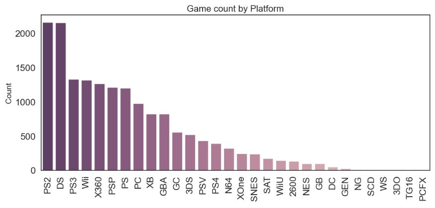
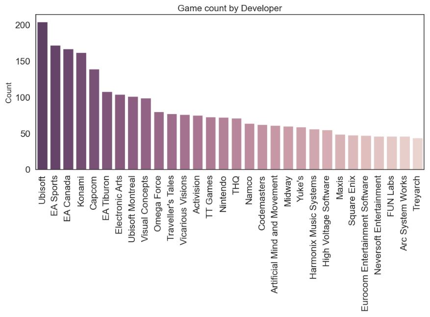
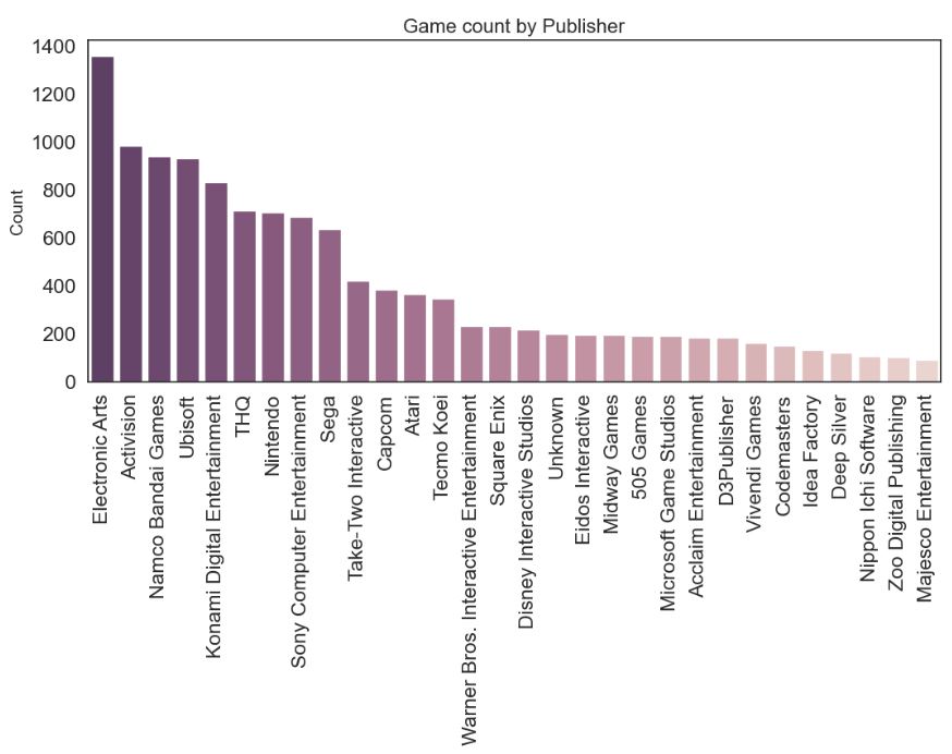
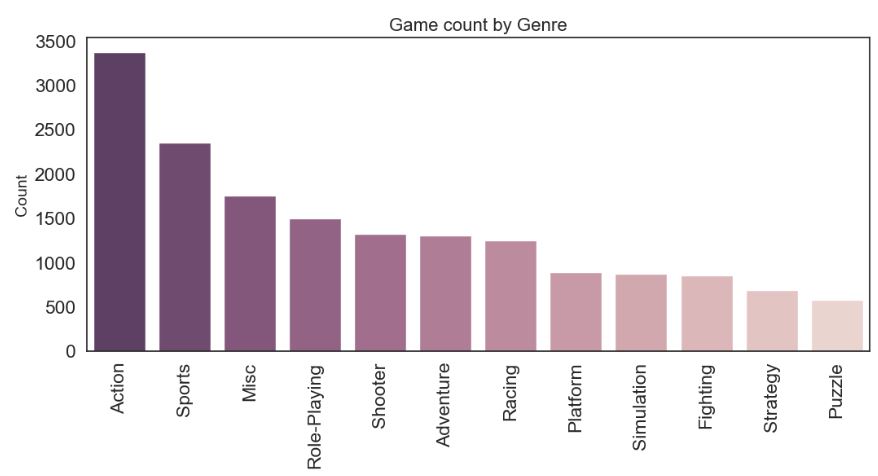
cols = [‘Platform’, ‘Developer’, ‘Publisher’, ‘Genre’]

for col in cols:
chart = df[[‘Name’, col]].groupby([col]).count().sort_values(‘Name’, ascending=False).reset_index()
sns.set_style(“white”)
plt.figure(figsize=(12.4, 5))
plt.xticks(rotation=90)
sns.barplot(x=col, y=’Name’, data=chart[:30], palette=sns.cubehelix_palette((12 if col == ‘Genre’ else 30), dark=0.3, light=.85, reverse=True)).set_title((‘Game count by ‘+col), fontsize=16)
plt.ylabel(‘Count’, fontsize=14)
plt.xlabel(”)

Let’s look at Critic_Score by defining the following 6 score groups

def score_group(score):
if score >= 90:
return ’90-100′
elif score >= 80:
return ’80-89′
elif score >= 70:
return ’70-79′
elif score >= 60:
return ’60-69′
elif score >= 50:
return ’50-59′
else:
return ‘0-49’

Let’s plot the following columns

cols = [‘Genre’, ‘Developer’, ‘Publisher’, ‘Platform’]

def in_top(x):
if x in pack:
return x
else:
pass
def width(x):
if x == ‘Platform’:
return 14.4
elif x == ‘Developer’:
return 13.2
elif x == ‘Publisher’:
return 11.3
elif x == ‘Genre’:
return 13.6

def height(x):
if x == ‘Genre’:
return 8
else:
return 9

sns.set(font_scale=1.5)
for col in cols:
pack = []
top = dfh[[‘Name’, col]].groupby([col]).count().sort_values(‘Name’, ascending=False).reset_index()[:15]
for x in top[col]:
pack.append(x)
dfh[col] = dfh[col].apply(lambda x: in_top(x))
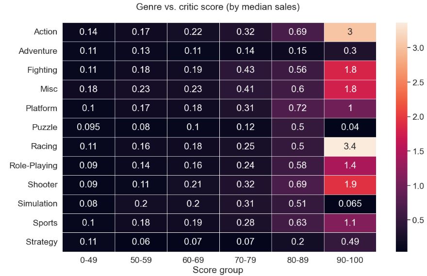
dfh_platform = dfh[[col, ‘Score_Group’, ‘Global_Sales’]].groupby([col, ‘Score_Group’]).median().reset_index().pivot(col, “Score_Group”, “Global_Sales”)
plt.figure(figsize=(width(col), height(col)))
sns.heatmap(dfh_platform, annot=True, fmt=”.2g”, linewidths=.5).set_title((‘ \n’+col+’ vs. critic score (by median sales) \n’), fontsize=18)
plt.ylabel(”, fontsize=14)
plt.xlabel(‘Score group \n’, fontsize=18)
pack = []

Feature Engineering & Correlations

Let’s plot the 6×6 correlation matrix

cols = [‘Platform’, ‘Genre’, ‘Publisher’, ‘Developer’, ‘Rating’]
for col in cols:
uniques = df[col].value_counts().keys()
uniques_dict = {}
ct = 0
for i in uniques:
uniques_dict[i] = ct
ct += 1

for k, v in uniques_dict.items():
    df.loc[df[col] == k, col] = v

df1 = df[[‘Platform’,’Genre’,’Publisher’,’Year_of_Release’,’Critic_Score’,’Global_Sales’]]
df1 = df1.dropna().reset_index(drop=True)
df1 = df1.astype(‘float64’)

mask = np.zeros_like(df1.corr())
sns.set(font_scale=1.5)
mask[np.triu_indices_from(mask)] = True
cmap = sns.diverging_palette(730, 300, sep=20, as_cmap=True, s=85, l=15, n=20)
with sns.axes_style(“white”):
fig, ax = plt.subplots(1,1, figsize=(15,8))
ax = sns.heatmap(df1.corr(), mask=mask, vmax=0.2, square=True, annot=True, fmt=”.3f”, cmap=cmap)

Let’s plot the linear trend Global_Sales vs Critic_Score

fig, ax = plt.subplots(1,1, figsize=(12,5))
sns.set(font_scale=2)
sns.regplot(x=”Critic_Score”, y=”Global_Sales”, data=df1.loc[df1.Year_of_Release >= 2014],
truncate=True, x_bins=15, color=”#75556c”).set(ylim=(0, 4), xlim=(50, 95))

ML Model Training & Validation

Let’s import the key libraries

from sklearn.preprocessing import LabelEncoder
from sklearn.model_selection import train_test_split
from sklearn.ensemble import RandomForestClassifier
from sklearn.calibration import CalibratedClassifierCV
from sklearn.model_selection import GridSearchCV
from sklearn.model_selection import StratifiedKFold
from sklearn.feature_selection import SelectFromModel
from sklearn.linear_model import LogisticRegression
from sklearn.metrics import classification_report, f1_score, accuracy_score, confusion_matrix
from sklearn import svm
from pandas import get_dummies

to prepare our data for ML

dfa = df
dfa = dfa.copy()
dfb = dfa[[‘Name’,’Platform’,’Genre’,’Publisher’,’Year_of_Release’,’Critic_Score’,’Global_Sales’]]
dfb = dfb.dropna().reset_index(drop=True)
df2 = dfb[[‘Platform’,’Genre’,’Publisher’,’Year_of_Release’,’Critic_Score’,’Global_Sales’]]
df2[‘Hit’] = df2[‘Global_Sales’]
df2.drop(‘Global_Sales’, axis=1, inplace=True)

def hit(sales):
if sales >= 1:
return 1
else:
return 0

df2[‘Hit’] = df2[‘Hit’].apply(lambda x: hit(x))

df_copy = pd.get_dummies(df2)

df3 = df_copy
y = df3[‘Hit’].values
df3 = df3.drop([‘Hit’],axis=1)
X = df3.values

It is time to split our data with test_size=0.30

Xtrain, Xtest, ytrain, ytest = train_test_split(X, y, test_size=0.30, random_state=200)

Let’s try RandomForestClassifier (RFC)

radm = RandomForestClassifier(random_state=200).fit(Xtrain, ytrain)
y_val_1 = radm.predict_proba(Xtest)
print(“Validation accuracy: “, sum(pd.DataFrame(y_val_1).idxmax(axis=1).values
== ytest)/len(ytest))

Validation accuracy:  0.8572025052192067

The Logistic Regression (LR) yields the similar result

log_reg = LogisticRegression().fit(Xtrain, ytrain)
y_val_2 = log_reg.predict_proba(Xtest)
print(“Validation accuracy: “, sum(pd.DataFrame(y_val_2).idxmax(axis=1).values
== ytest)/len(ytest))

Validation accuracy:  0.8576200417536535

The LR classification report is

all_predictions = log_reg.predict(Xtest)
print(classification_report(ytest, all_predictions))

 precision    recall  f1-score   support

           0       0.88      0.97      0.92      1989
           1       0.66      0.33      0.44       406

    accuracy                           0.86      2395
   macro avg       0.77      0.65      0.68      2395
weighted avg       0.84      0.86      0.84      2395

The LR normalized confusion matrix is

cm = confusion_matrix(ytest, all_predictions)
sns.set(font_scale=2)
target_names=[‘0′,’1’]

cmn = cm.astype(‘float’) / cm.sum(axis=1)[:, np.newaxis]
fig, ax = plt.subplots(figsize=(10,10))
sns.heatmap(cmn, annot=True, fmt=’.2f’, xticklabels=target_names, yticklabels=target_names)
plt.ylabel(‘Actual’)
plt.xlabel(‘Predicted’)
plt.show(block=False)

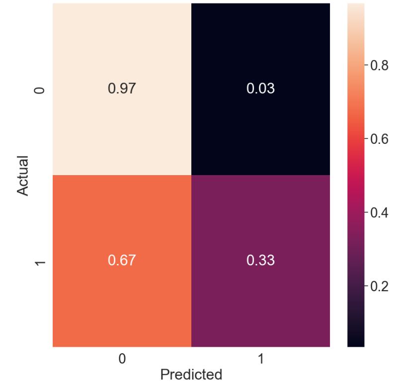
High recall for target_class=0 means that an algorithm returns most of the relevant results for this class with FN=3%. This algorithm is not suitable for detecting target_class=1.

SMOTE Data Resampling

Let’s perform the SMOTE data resampling

import imblearn
print(imblearn.version)

0.9.1

from imblearn.over_sampling import SMOTE
sm = SMOTE(random_state=42)
X_res, y_res = sm.fit_resample(Xtrain, ytrain)

log_reg = LogisticRegression().fit(X_res, y_res)
y_val_2 = log_reg.predict_proba(Xtest)
print(“Validation accuracy: “, sum(pd.DataFrame(y_val_2).idxmax(axis=1).values
== ytest)/len(ytest))

Validation accuracy:  0.7766179540709812

all_predictions = log_reg.predict(Xtest)
print(classification_report(ytest, all_predictions))

precision    recall  f1-score   support

           0       0.94      0.78      0.85      1989
           1       0.41      0.77      0.54       406

    accuracy                           0.78      2395
   macro avg       0.68      0.78      0.70      2395
weighted avg       0.85      0.78      0.80      2395

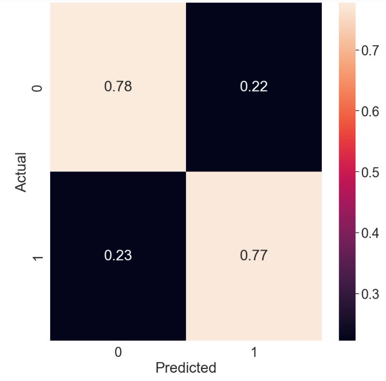
Let’s plot the LR normalized confusion matrix

cm = confusion_matrix(ytest, all_predictions)
sns.set(font_scale=2)
target_names=[‘0′,’1’]

cmn = cm.astype(‘float’) / cm.sum(axis=1)[:, np.newaxis]
fig, ax = plt.subplots(figsize=(10,10))
sns.heatmap(cmn, annot=True, fmt=’.2f’, xticklabels=target_names, yticklabels=target_names)
plt.ylabel(‘Actual’)
plt.xlabel(‘Predicted’)
plt.show(block=False)

let’s print the feature ranking
print(‘Feature ranking (top 10):’)

for f in range(10):
print(‘%d. feature %d %s (%f)’ % (f+1 , indices[f], df3.columns[indices[f]],
radm.feature_importances_[indices[f]]))

Feature ranking (top 10):
1. feature 1 Critic_Score (0.338061)
2. feature 0 Year_of_Release (0.162324)
3. feature 216 Publisher_Nintendo (0.031328)
4. feature 99 Publisher_Electronic Arts (0.022656)
5. feature 19 Genre_Action (0.018284)
6. feature 27 Genre_Shooter (0.016449)
7. feature 29 Genre_Sports (0.016447)
8. feature 9 Platform_PS2 (0.016164)
9. feature 7 Platform_PC (0.014517)
10. feature 42 Publisher_Activision (0.014068)

It is clear that Critic_Score is the most dominant feature to be considered.

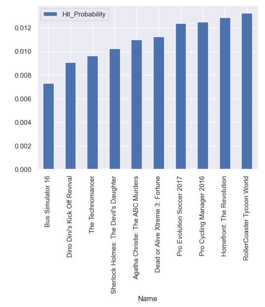
Let’s plot the LR high/low hit probability

not_hit_copy = df_copy[df_copy[‘Hit’] == 0]
df4 = not_hit_copy
y = df4[‘Hit’].values
df4 = df4.drop([‘Hit’],axis=1)
X = df4.values

pred = log_reg.predict_proba(X)

dfb = dfb[dfb[‘Global_Sales’] < 1]

dfb[‘Hit_Probability’] = pred[:,1]

dfb = dfb[dfb[‘Year_of_Release’] == 2016]
dfb.sort_values([‘Hit_Probability’], ascending=[False], inplace=True)
dfb = dfb[[‘Name’, ‘Platform’, ‘Hit_Probability’]]

dfmax=dfb[:10].reset_index(drop=True)

dfmin=dfb[:-11:-1].reset_index(drop=True)

sns.set(font_scale=1)
dfmax.plot.bar(x=’Name’, y=’Hit_Probability’)

High Hit Probability

Low Hit Probability

sns.set(font_scale=1)
dfmin.plot.bar(x=’Name’, y=’Hit_Probability’)

Hyper-Parameter Optimization

Let’s consider GridSearchCV

from sklearn.model_selection import GridSearchCV
model = LogisticRegression()
grid_vals = {‘penalty’: [‘l1′,’l2’], ‘C’: [0.001,0.01,0.1,1]}
grid_lr = GridSearchCV(estimator=model, param_grid=grid_vals, scoring=’accuracy’,
cv=6, refit=True, return_train_score=False)

Training and Prediction:

grid_lr.fit(X_res, y_res)
preds = grid_lr.best_estimator_.predict(Xtest)

print(classification_report(ytest, preds))

 precision    recall  f1-score   support

           0       0.94      0.78      0.85      1989
           1       0.41      0.77      0.54       406

    accuracy                           0.78      2395
   macro avg       0.68      0.78      0.70      2395
weighted avg       0.85      0.78      0.80      2395

Let’s apply RandomizedSearchCV

from sklearn.model_selection import RandomizedSearchCV
model = RandomForestClassifier()
param_vals = {‘max_depth’: [200, 500, 800, 1100], ‘n_estimators’: [100, 200, 300, 400]
}
random_rf = RandomizedSearchCV(estimator=model, param_distributions=param_vals,
n_iter=10, scoring=’accuracy’, cv=5,
refit=True, n_jobs=-1)

Training and prediction:

random_rf.fit(X_res, y_res)
preds = random_rf.best_estimator_.predict(Xtest)

print(classification_report(ytest, preds))

precision    recall  f1-score   support

           0       0.89      0.94      0.91      1989
           1       0.59      0.44      0.50       406

    accuracy                           0.85      2395
   macro avg       0.74      0.69      0.71      2395
weighted avg       0.84      0.85      0.84      2395

Let’s apply TPOTClassifier

tpot_clf = TPOTClassifier(generations=10, population_size=10,
verbosity=2, offspring_size=10, scoring=’accuracy’, cv=6)

Training and prediction:

tpot_clf.fit(X_res, y_res)
tpot_pred = tpot_clf.score(Xtest, ytest)

Optimization Progress:   0%|          | 0/110 [00:00<?, ?pipeline/s]

Generation 1 - Current best internal CV score: 0.9001460036188931

Generation 2 - Current best internal CV score: 0.9146615780315163

Generation 3 - Current best internal CV score: 0.9157356682819965

Generation 4 - Current best internal CV score: 0.9157356682819965

Generation 5 - Current best internal CV score: 0.9157356682819965

Generation 6 - Current best internal CV score: 0.9186396566904459

Generation 7 - Current best internal CV score: 0.9191783310108637

Generation 8 - Current best internal CV score: 0.9191783310108637

Generation 9 - Current best internal CV score: 0.9191783310108637

Generation 10 - Current best internal CV score: 0.9191783310108637

Best pipeline: RandomForestClassifier(input_matrix, bootstrap=False, criterion=gini, max_features=0.2, min_samples_leaf=3, min_samples_split=6, n_estimators=100)

print(classification_report(ytest, preds))

 precision    recall  f1-score   support

           0       0.89      0.94      0.91      1989
           1       0.59      0.44      0.50       406

    accuracy                           0.85      2395
   macro avg       0.74      0.69      0.71      2395
weighted avg       0.84      0.85      0.84      2395

Summary

• Most popular platforms are PS2, DS, and PS3.
• Most popular game developers are Ubisoft, EA Sports, and EA Canada.
• Most popular publishers are Electronic Arts, Activision, and Namco Bandai Games.
• Action, Sports, and RPG are among the most popular genres.
• Genre vs max critic score 90-100: Action and Racing.
• Developer vs max critic score 90-100: Capcom, Electronic Arts, and Ubisoft Montreal.
• Publisher vs max critic score 90-100: Microsoft Game Studios, Sony Computer Entertainment, and Warner Bros. Interactive Entertainment.
• Platform vs max critic score 90-100: X360, 3DS, PS, PS2, PS3, and PSP.
• The correlation matrix shows very little correlation between variables, except the moderate correlation of 0.245 between Global_Sales and Critic_Score.
• Critic_Score is the most dominant feature in the trained ML model.
• Logistic Regression (LR) yields f1-score = 0.97 to detect class=0 with FP=0.03
• LR with SMOTE data resampling yields FP=0.22 and FN=0.23.
• Hyperparameter optimization does not improve ML results in terms of key metrics discussed above.
• We have predicted top 10 video games with highest/lowest hit probabilities.

Explore More

• An Overview of Video Games in 2023: Trends, Technology, and Market Research
• Customer Reviews NLP Spacy Analysis and ML/AI Demand Forecasting of the Steam PC Video Game Service
• Video Game Sales Data Visualization, Wrangling and Market Analysis in Python

Do-Follow Socials