Customer Reviews NLP Spacy Analysis and ML/AI Demand Forecasting of the Steam PC Video Game Service

• Steam is a video game digital distribution service and storefront from Valve.
• The service is the largest digital distribution platform for PC gaming. 2022 has already seen over 6000 new games released on Steam. That’s over 34 games a day.
• Referring to the two public-domain datasets steam_reviews.csv and steam_games.csv, the goal of this post is to perform the comprehensive customer reviews NLP Spacy sentiment analysis and ML/AI demand forecasting of the Steam PC video game service.

Exploratory Data Analysis (EDA)

Let’s set the working directory YOURPATH

import os

os.chdir(‘YOURPATH’)

os. getcwd()

and import the basic libraries

import numpy as np
import pandas as pd
import matplotlib.pyplot as plt
import seaborn as sns

Let’s read the first dataset

df=pd.read_csv(‘steam_games.csv’, comment=’\”‘)
df.info()

<class 'pandas.core.frame.DataFrame'>
RangeIndex: 40833 entries, 0 to 40832
Data columns (total 20 columns):
 #   Column                    Non-Null Count  Dtype  
---  ------                    --------------  -----  
 0   url                       40833 non-null  object 
 1   types                     40831 non-null  object 
 2   name                      40817 non-null  object 
 3   desc_snippet              27612 non-null  object 
 4   recent_reviews            2706 non-null   object 
 5   all_reviews               28470 non-null  object 
 6   release_date              37654 non-null  object 
 7   developer                 40490 non-null  object 
 8   publisher                 35733 non-null  object 
 9   popular_tags              37888 non-null  object 
 10  game_details              40313 non-null  object 
 11  languages                 40797 non-null  object 
 12  achievements              12194 non-null  float64
 13  genre                     40395 non-null  object 
 14  game_description          37920 non-null  object 
 15  mature_content            2897 non-null   object 
 16  minimum_requirements      21069 non-null  object 
 17  recommended_requirements  21075 non-null  object 
 18  original_price            35522 non-null  object 
 19  discount_price            14543 non-null  object 
dtypes: float64(1), object(19)
memory usage: 6.2+ MB

Let’s plot Average Common Name

sorted_genres = pd.value_counts(np.array(df[‘name’]))
sorted_genres = sorted_genres.sort_values(ascending=False)
print(“Series Size “, sorted_genres.size)
print(“Average Common Name “, sorted_genres.mean())

genre_slice = sorted_genres.head(10)
labels = genre_slice.keys()

fig, ax = plt.subplots()
plt.title(‘name’)
pchart = ax.pie(genre_slice, labels = labels, autopct=’%1.1f%%’)

Series Size  40749
Average Common Name  1.001668752607426

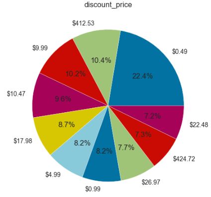
Let’s plot Average Common Discount Price

sorted_genres = pd.value_counts(np.array(df[‘discount_price’]))
sorted_genres = sorted_genres.sort_values(ascending=False)
print(“Series Size “, sorted_genres.size)
print(“Average Common Discount Price “, sorted_genres.mean())

genre_slice = sorted_genres.head(10)
labels = genre_slice.keys()

fig, ax = plt.subplots()
plt.title(‘discount_price’)
pchart = ax.pie(genre_slice, labels = labels, autopct=’%1.1f%%’)

Series Size  2060
Average Common Discount Price  7.059708737864078

Let’s plot Average Common Developer

sorted_genres = pd.value_counts(np.array(df[‘developer’]))
sorted_genres = sorted_genres.sort_values(ascending=False)
print(“Series Size “, sorted_genres.size)
print(“Average Common Developer “, sorted_genres.mean())

genre_slice = sorted_genres.head(10)
labels = genre_slice.keys()

fig, ax = plt.subplots()
plt.title(‘developer’)
pchart = ax.pie(genre_slice, labels = labels, autopct=’%1.1f%%’)

Series Size  17420
Average Common Developer  2.3243398392652126

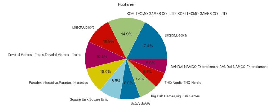
Let’s plot Average Common Publisher

sorted_genres = pd.value_counts(np.array(df[‘publisher’]))
sorted_genres = sorted_genres.sort_values(ascending=False)
print(“Series Size “, sorted_genres.size)
print(“Average Common Publisher “, sorted_genres.mean())

genre_slice = sorted_genres.head(10)
labels = genre_slice.keys()

fig, ax = plt.subplots()
plt.title(‘Publisher’)
pchart = ax.pie(genre_slice, labels = labels, autopct=’%1.1f%%’)

Series Size  15290
Average Common Publisher  2.3370176586003923

Let’s plot Most Reviewed Game Tags

sorted_genres = pd.value_counts(np.array(df[‘popular_tags’]))
sorted_genres = sorted_genres.sort_values(ascending=False)
print(“Series Size “, sorted_genres.size)
print(“Average Common Genres “, sorted_genres.mean())

genre_slice = sorted_genres.head(10)
labels = genre_slice.keys()

fig, ax = plt.subplots()
plt.title(‘Most Reviewed Game Tags’)
pchart = ax.pie(genre_slice, labels = labels, autopct=’%1.1f%%’)

Series Size  20852
Average Common Genres  1.816995971609438

Let’s import the libraries and load the second dataset

import pandas as pd
import numpy as np
import matplotlib.pyplot as plt
%matplotlib inline
import seaborn as sns

import spacy

data = pd.read_csv(“steam_reviews.csv”)

Let’s group and plot top 10 reviews

data[‘review_length’] = data.apply(lambda row: len(str(row[‘review’])), axis=1)

data[‘recommendation_int’] = data[‘recommendation’] == ‘Recommended’
data[‘recommendation_int’] = data[‘recommendation_int’].astype(int)

reviews_count = data.groupby([‘title’])[‘review’].count().sort_values(ascending=False)

reviews_count = reviews_count.reset_index()

sns.set(style=”darkgrid”)
sns.set(font_scale=3)
plt.figure(figsize=(25,20))
sns.barplot(y=reviews_count[‘title’], x=reviews_count[‘review’], data=reviews_count,
label=”Total”, color=”r”)

reviews_count_pos = data.groupby([‘title’, ‘recommendation_int’])[‘review’].count().sort_values(ascending=False)
reviews_count_pos = reviews_count_pos.reset_index()
reviews_count_pos = reviews_count_pos[reviews_count_pos[‘recommendation_int’] == 1]
sns.barplot(y=’title’, x=’review’, data=reviews_count_pos.nlargest(10, ‘review’),
label=”Total”, color=”b”)

Let’s group data by recommendation_int as

data.groupby([‘title’, ‘recommendation_int’])[‘review’].count()

Let’s plot recommendation_int

polarity_count = data.groupby([‘recommendation_int’]).count()
polarity_count = polarity_count.reset_index()

sns.set(font_scale=1)
ax = sns.barplot(x=polarity_count[‘recommendation_int’], y=polarity_count[‘review’],
data=polarity_count, hue=’recommendation_int’)

NLP Spacy Analysis & ML/AI Pipeline

Let’s clean, split and train the second dataset as follows:

clean_data = data.dropna()

train = clean_data[clean_data[‘title’] == ‘Grand Theft Auto V’]

X = train[‘review’]
y = train[‘recommendation_int’]

from sklearn.model_selection import train_test_split

X_train, X_test, y_train, y_test = train_test_split(X, y, test_size=0.2, random_state=273, stratify=y)

en_nlp = spacy.load(“en_core_web_sm”)
spacy_tokenizer = en_nlp.tokenizer

def custom_tokenizer(document):
doc_spacy = en_nlp(document)
return [token.lemma_ for token in doc_spacy]

from time import time

from sklearn.linear_model import LogisticRegression

from sklearn.feature_extraction.text import CountVectorizer
from sklearn.feature_extraction.text import TfidfVectorizer

from sklearn.pipeline import Pipeline
from sklearn.metrics import classification_report

t0 = time()
text_clf = Pipeline([
(‘vect’, TfidfVectorizer(max_df=0.99, norm=’l2′)),
(‘clf’, LogisticRegression(solver=’saga’, fit_intercept=True, class_weight=’balanced’, C=0.1))
])
print(“preprocessing done in %0.3fs.” % (time() – t0))

t0 = time()
text_clf.fit(X_train, y_train)
print(“fitting done in %0.3fs.” % (time() – t0))

t0 = time()
y_pred = text_clf.predict(X_test)
print(“predicting done in %0.3fs.” % (time() – t0))

print(classification_report(y_test, y_pred)) #, target_names=target_names))

preprocessing done in 0.000s.
fitting done in 2.310s.
predicting done in 0.393s.
              precision    recall  f1-score   support

           0       0.82      0.84      0.83      8173
           1       0.88      0.87      0.88     11763

    accuracy                           0.86     19936
   macro avg       0.85      0.85      0.85     19936
weighted avg       0.86      0.86      0.86     19936

Model Validation

Let’s import the following libraries

import scikitplot as skplt

import sklearn

from sklearn.model_selection import train_test_split

from sklearn.ensemble import RandomForestClassifier, RandomForestRegressor, GradientBoostingClassifier, ExtraTreesClassifier
from sklearn.linear_model import LinearRegression, LogisticRegression
from sklearn.cluster import KMeans
from sklearn.decomposition import PCA

import matplotlib.pyplot as plt

import sys
import warnings
warnings.filterwarnings(“ignore”)

print(“Scikit Plot Version : “, skplt.version)
print(“Scikit Learn Version : “, sklearn.version)
print(“Python Version : “, sys.version)

%matplotlib inline

cikit Plot Version :  0.3.7
Scikit Learn Version :  1.2.2
Python Version :  3.9.16 (main, Jan 11 2023, 16:16:36) [MSC v.1916 64 bit (AMD64)]

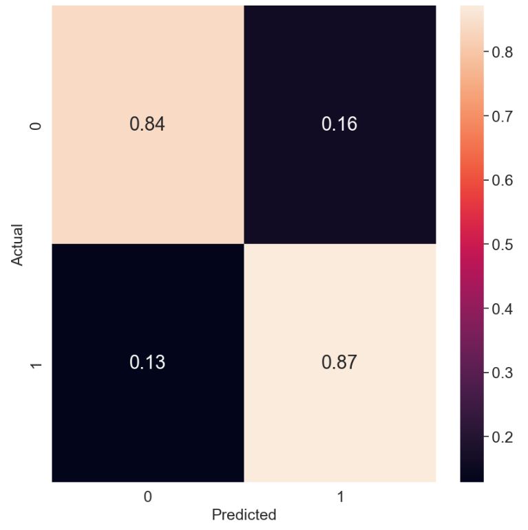
Let’s plot the normalized confusion matrix

from sklearn.metrics import confusion_matrix
import seaborn as sns
cm = confusion_matrix(y_test, y_pred)
target_names=[‘0′,’1’]

cmn = cm.astype(‘float’) / cm.sum(axis=1)[:, np.newaxis]
fig, ax = plt.subplots(figsize=(10,10))
sns.heatmap(cmn, annot=True, fmt=’.2f’, xticklabels=target_names, yticklabels=target_names)
plt.ylabel(‘Actual’,fontsize=18)
plt.xlabel(‘Predicted’,fontsize=18)
plt.rcParams.update({‘font.size’: 22})
SMALL_SIZE=24
plt.rc(‘xtick’, labelsize=SMALL_SIZE) # fontsize of the tick labels
plt.rc(‘ytick’, labelsize=SMALL_SIZE) # fontsize of the tick labels
plt.rc(‘legend’, fontsize=SMALL_SIZE) # legend fontsize
plt.show(block=False)

Let’s plot the Logistic Regression (LR) ROC Curve

Y_test_probs = text_clf.predict_proba(X_test)

skplt.metrics.plot_roc_curve(y_test, Y_test_probs,
title=”LR ROC Curve”, figsize=(12,6));

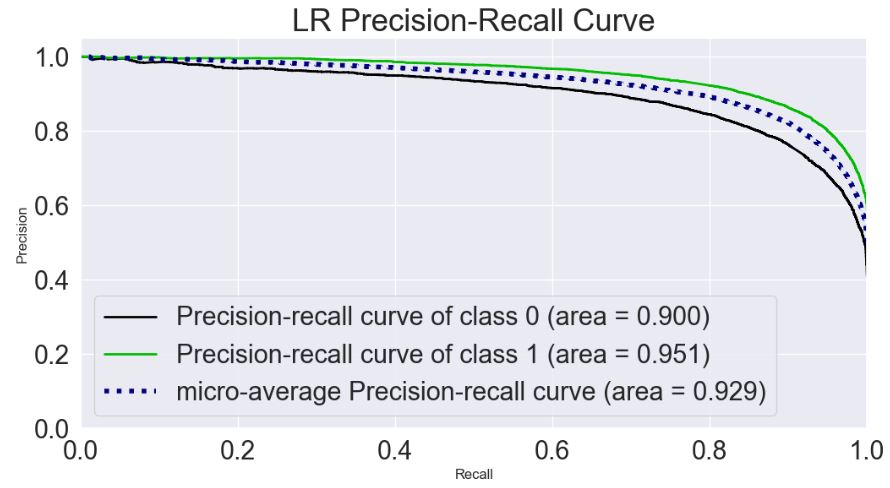
Let’s plot the LR Precision-Recall Curve

skplt.metrics.plot_precision_recall_curve(y_test, Y_test_probs,
title=”LR Precision-Recall Curve”, figsize=(12,6));

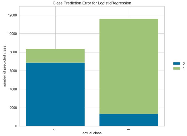
Let’s plot the class prediction error for LR

from yellowbrick.classifier import ClassPredictionError

viz = ClassPredictionError(text_clf,
classes=target_names,
fig=plt.figure(figsize=(9,6)))

viz.fit(X_train, y_train)

viz.score(X_test, y_test)

viz.show();

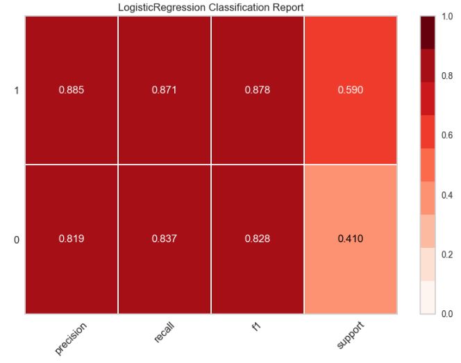
Let’s plot the classification report for LR

from yellowbrick.classifier.classification_report import classification_report

classification_report(text_clf,
X_train, y_train,
X_test, y_test,
classes=target_names,
support=”percent”,
cmap=”Reds”,
font_size=16,
fig=plt.figure(figsize=(8,6))
);

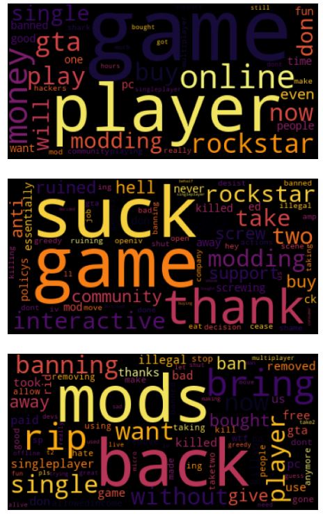
NLP Word Clouds

Here we want to find out why customers who left negative reviews for certain products are not satisfied.

clean_data = data.dropna()

train = clean_data[(clean_data[‘title’] == ‘Grand Theft Auto V’) & (clean_data[‘recommendation_int’] == 0)]

X = train[‘review’]
y = train[‘recommendation_int’]

from sklearn.model_selection import train_test_split

X_train, X_test, y_train, y_test = train_test_split(X, y, test_size=0.2, random_state=273, stratify=y)

from wordcloud import WordCloud, STOPWORDS

def print_top_words(model, feature_names, n_top_words, colormap=’viridis’):
for topic_idx, topic in enumerate(model.components_):

    message = " ".join([feature_names[i]
                         for i in topic.argsort()[:-n_top_words - 1:-1]])


    generate_wordcloud(message, colormap)
print()    

def generate_wordcloud(text, colormap=’viridis’):
wordcloud = WordCloud(
relative_scaling = 1.0,
colormap = colormap
).generate(text)
plt.imshow(wordcloud)
plt.axis(“off”)
plt.show()

Let’s apply the NMF decomposition with n_components=5

from sklearn.decomposition import NMF

tfidf_vect = TfidfVectorizer(max_df=.50)

X_train_topical = tfidf_vect.fit_transform(X_train)

nmf = NMF(n_components=5, random_state=273,
l1_ratio=.5)

document_topics_nmf = nmf.fit_transform(X_train_topical)

Let’s get topic contents and visualize the topics for negative reviews

from sklearn.feature_extraction.text import TfidfVectorizer
tfidf_vect = TfidfVectorizer(max_df=.50)
X_train_topical = tfidf_vect.fit_transform(X_train)
tfidf_vect_feature_names=tfidf_vect.get_feature_names_out()
print_top_words(nmf, tfidf_vect_feature_names, 100, colormap=’inferno’)

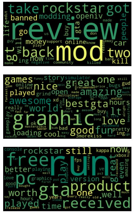
Here’s another data setup for topic modeling, but for different example:
extract topics from positive reviews using LDA with n_components=5

from sklearn.decomposition import LatentDirichletAllocation

vect = CountVectorizer(max_features=10000, max_df=.20)
X_train_topical = vect.fit_transform(X_train)

lda = LatentDirichletAllocation(n_components=5, learning_method=”batch”,
max_iter=25, random_state=273)

vect_feature_names = vect.get_feature_names_out()
print_top_words(lda, vect_feature_names, 100, colormap=’summer’)

Summary

• Online user reviews remain a rich yet underexplored resource for collecting feedback about game experience for the video game industry.
• In this post, we have examined the Steam platform that has has an extensive library of PC video games ranging from a multitude of genres, also referred to as “tags”.
• We have employed NLP analytics to automatically elicit components of the game experience from online reviews and examined each component’s relative importance to user satisfaction. 
• ML/AI for NLP has been applied on online text reviews for predicting factors such as the helpfulness of a review, success/popularity of a product based on reviews, along with other factors that may influence a user’s behavior and increase profitability of a product.
• We have implemented the Tfidf logistic regression and demonstrated its use in modeling data from a business process involving customer feedback.
• We have applied and compared the NMF and LDA topic modelling techniques.
• Results can be used as guidance for game evaluation, marketing strategy, and new game development.
• Future works could include acquiring information such as purchasing patterns, content usage, historical price changes, and patterns of individual games.

Explore More

• Video Game Sales Data Visualization, Wrangling and Market Analysis in Python

• Trending YouTube Video Data Science, NLP Predictions & Sentiment Analysis