
Photo by CardMapr.nl on Unsplash
- In 2023, global card industry losses to fraud are projected to reach $36.13 bln, or $0.0668 per $100 of volume.
- Enhancing credit card fraud detection is therefore a top priority for all banks and financial organizations.
- Thanks to AI-based techniques, credit card fraud detection (CCFD) is becoming easier and more accurate. AI models can recognise unusual credit card transactions and fraud. CCFD involves collecting and sorting raw data, which is then used to train the model to predict the probability of fraud.
- AI allows for creating algorithms that process large datasets with many variables and help find these hidden correlations between user behavior and the likelihood of fraudulent actions. Another strength of AI systems compared to rule-based ones is faster data processing and less manual work.
- Inspired by the recent study, our Python CCFD AI project aims to create an improved binary classifier that can recognize fraudulent credit card transactions with a high degree of confidence.
- Specifically, we have conducted a comparative analysis of the available supervised Machine Learning (ML) and Deep Learning (DL) techniques for CCFD.
- In this post, we will discuss a multiple-model ML/DL approach that closely resembles ensemble learning. An ensemble learning method involves combining the predictions from multiple contributing models.
- In addition, we will compare multiple techniques to determine the best performing model in detecting fraudulent transactions in terms of scikit-learn metrics and scoring to quantify the quality of CCFD predictions.
- Conventionally, we use the open-source Kaggle dataset that contains transactions made by credit cards in September 2013 by European cardholders. These are anonymized credit card transactions labeled as fraudulent (1) or genuine (0). The dataset is highly unbalanced, the positive class (frauds) account for 0.172% of all transactions.
- Read more: Dal Pozzolo, Andrea; Boracchi, Giacomo; Caelen, Olivier; Alippi, Cesare; Bontempi, Gianluca. Credit card fraud detection: a realistic modeling and a novel learning strategy, IEEE transactions on neural networks and learning systems,29,8,3784-3797,2018,IEEE
Clickable Table of Contents
- Data Preparation & Exploratory Analysis
- Keras ANN Model Training & Validation
- Multiple-Model Training & Validation
- Multiple-Model ML/DL F1-Score Comparison
- Best ML/DL Model Performance QC Analysis
- K-Means PCA Clusters & Variance Analysis
- Final XGBoost Classification Report
- Summary
- Explore More
Data Preparation & Exploratory Analysis
Let’s set the working directory
import os
os.chdir(‘YOURPATH’)
os. getcwd()
and import the necessary packages
import pandas as pd
import numpy as np
import matplotlib.pyplot as plt
import seaborn as sns
%matplotlib inline
sns.set_style(“whitegrid”)
Let’s load the dataset from the csv file using Pandas
data = pd.read_csv(“creditcard.csv”)
data.head()
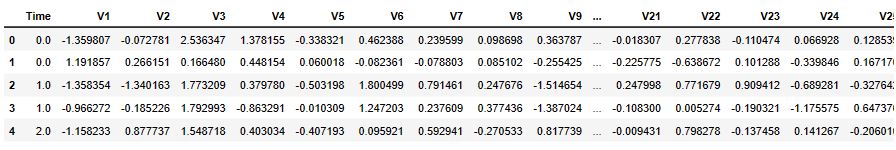
(5 rows × 31 columns)
Here, features V1, V2, … V28 are the principal components obtained with PCA, the only features which have not been transformed with PCA are ‘Time’ and ‘Amount’. Feature ‘Time’ contains the seconds elapsed between each transaction and the first transaction in the dataset. The feature ‘Amount’ is the transaction Amount, this feature can be used for example-dependant cost-sensitive learning. Feature ‘Class’ is the response variable and it takes value 1 in case of fraud and 0 otherwise.
Describing the Input Data:
data.info()
<class 'pandas.core.frame.DataFrame'>
RangeIndex: 284807 entries, 0 to 284806
Data columns (total 31 columns):
 #   Column  Non-Null Count   Dtype
---  ------  --------------   -----
 0   Time    284807 non-null  float64
 1   V1      284807 non-null  float64
 2   V2      284807 non-null  float64
 3   V3      284807 non-null  float64
 4   V4      284807 non-null  float64
 5   V5      284807 non-null  float64
 6   V6      284807 non-null  float64
 7   V7      284807 non-null  float64
 8   V8      284807 non-null  float64
 9   V9      284807 non-null  float64
 10  V10     284807 non-null  float64
 11  V11     284807 non-null  float64
 12  V12     284807 non-null  float64
 13  V13     284807 non-null  float64
 14  V14     284807 non-null  float64
 15  V15     284807 non-null  float64
 16  V16     284807 non-null  float64
 17  V17     284807 non-null  float64
 18  V18     284807 non-null  float64
 19  V19     284807 non-null  float64
 20  V20     284807 non-null  float64
 21  V21     284807 non-null  float64
 22  V22     284807 non-null  float64
 23  V23     284807 non-null  float64
 24  V24     284807 non-null  float64
 25  V25     284807 non-null  float64
 26  V26     284807 non-null  float64
 27  V27     284807 non-null  float64
 28  V28     284807 non-null  float64
 29  Amount  284807 non-null  float64
 30  Class   284807 non-null  int64
dtypes: float64(30), int64(1)
memory usage: 67.4 MB
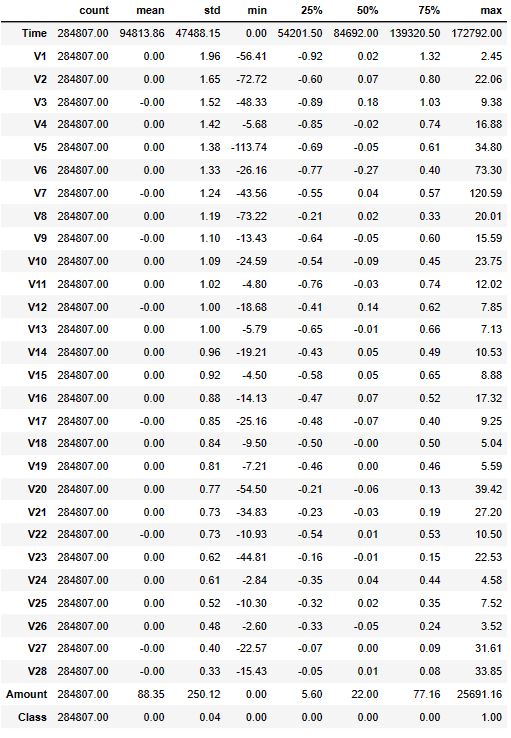
pd.set_option(“display.float”, “{:.2f}”.format)
data.describe().T
Let us now check the missing values in the dataset
data.isnull().sum().sum()
0
data.columns
Index(['Time', 'V1', 'V2', 'V3', 'V4', 'V5', 'V6', 'V7', 'V8', 'V9', 'V10',
       'V11', 'V12', 'V13', 'V14', 'V15', 'V16', 'V17', 'V18', 'V19', 'V20','V21', 'V22', 'V23', 'V24', 'V25', 'V26', 'V27', 'V28', 'Amount',
       'Class'], dtype='object')
Let’s look at the Transaction Class Distribution
LABELS = [“Normal”, “Fraud”]
count_classes = pd.value_counts(data[‘Class’], sort = True)
count_classes.plot(kind = ‘bar’, rot=0)
plt.title(“Transaction Class Distribution”)
plt.xticks(range(2), LABELS)
plt.xlabel(“Class”)
plt.ylabel(“Frequency”);

data.Class.value_counts()
Class
0    284315
1       492
Name: count, dtype: int64
data.Class.value_counts(normalize=True).mul(100).round(3).astype(str) + ‘%’
Class
0    99.827%
1     0.173%
Name: proportion, dtype: object
It appears that most of the transactions are non-fraud. Only 0.173% fraudulent transaction out all the transactions. The data is highly unbalanced.
Let’s separate fraud and normal data
fraud = data[data[‘Class’]==1]
normal = data[data[‘Class’]==0]
print(f”Shape of Fraudulent transactions: {fraud.shape}”)
print(f”Shape of Non-Fraudulent transactions: {normal.shape}”)
Shape of Fraudulent transactions: (492, 31)
Shape of Non-Fraudulent transactions: (284315, 31)
Let’s compare Amount fraud vs normal data
pd.concat([fraud.Amount.describe(), normal.Amount.describe()], axis=1)

Let’s compare Time fraud vs normal data
pd.concat([fraud.Time.describe(), normal.Time.describe()], axis=1)

Let's look at the feature heatmap to find any high correlations
plt.figure(figsize=(10,10))
sns.heatmap(data=data.corr(), cmap=”seismic”)
plt.show();

The correlation matrix graphically gives us an idea of how features correlate with each other and can help us predict what are the features that are most relevant for the prediction. It is clear that most of the features do not correlate to other features but there are some features that either has a positive or a negative correlation with each other. For example, V2 and V5 are highly negatively correlated with the Amount.
Finally, let’s divide the data into features and target variables. In addition, we will be dividing the dataset into two main groups: one for training the model and the other for testing our trained model’s performance:
from sklearn.model_selection import train_test_split
from sklearn.preprocessing import StandardScaler
scalar = StandardScaler()
X = data.drop(‘Class’, axis=1)
y = data.Class
X_train_v, X_test, y_train_v, y_test = train_test_split(X, y,
test_size=0.3, random_state=42)
X_train, X_validate, y_train, y_validate = train_test_split(X_train_v, y_train_v,
test_size=0.2, random_state=42)
X_train = scalar.fit_transform(X_train)
X_validate = scalar.transform(X_validate)
X_test = scalar.transform(X_test)
w_p = y_train.value_counts()[0] / len(y_train)
w_n = y_train.value_counts()[1] / len(y_train)
print(f”Fraudulant transaction weight: {w_n}”)
print(f”Non-Fraudulant transaction weight: {w_p}”)
Fraudulant transaction weight: 0.0017994745785028623
Non-Fraudulant transaction weight: 0.9982005254214972
print(f”TRAINING: X_train: {X_train.shape}, y_train: {y_train.shape}\n{‘’55}”) print(f”VALIDATION: X_validate: {X_validate.shape}, y_validate: {y_validate.shape}\n{”50}”)
print(f”TESTING: X_test: {X_test.shape}, y_test: {y_test.shape}”)
TRAINING: X_train: (159491, 30), y_train: (159491,)
_______________________________________________________
VALIDATION: X_validate: (39873, 30), y_validate: (39873,)
__________________________________________________
TESTING: X_test: (85443, 30), y_test: (85443,)
We will need the following function to print the model score
from sklearn.metrics import accuracy_score, confusion_matrix, classification_report, f1_score
def print_score(label, prediction, train=True):
if train:
clf_report = pd.DataFrame(classification_report(label, prediction, output_dict=True))
print(“Train Result:\n================================================”)
print(f”Accuracy Score: {accuracy_score(label, prediction) * 100:.2f}%”)
print(“___________________________________“)
print(f”Classification Report:\n{clf_report}”)
print(“___________________________________“)
print(f”Confusion Matrix: \n {confusion_matrix(y_train, prediction)}\n”)
elif train==False:
    clf_report = pd.DataFrame(classification_report(label, prediction, output_dict=True))
    print("Test Result:\n================================================")
    print(f"Accuracy Score: {accuracy_score(label, prediction) * 100:.2f}%")
    print("_______________________________________________")
    print(f"Classification Report:\n{clf_report}")
    print("_______________________________________________")
    print(f"Confusion Matrix: \n {confusion_matrix(label, prediction)}\n")
Keras ANN Model Training & Validation
Let’s define the following Artificial Neural Network (ANN) model
from tensorflow import keras
model = keras.Sequential([
keras.layers.Dense(256, activation=’relu’, input_shape=(X_train.shape[-1],)),
keras.layers.BatchNormalization(),
keras.layers.Dropout(0.3),
keras.layers.Dense(256, activation=’relu’),
keras.layers.BatchNormalization(),
keras.layers.Dropout(0.3),
keras.layers.Dense(256, activation=’relu’),
keras.layers.BatchNormalization(),
keras.layers.Dropout(0.3),
keras.layers.Dense(1, activation=’sigmoid’),
])
model.summary()
Model: "sequential"
_________________________________________________________________
 Layer (type)                Output Shape              Param #
=================================================================
 dense (Dense)               (None, 256)               7936

 batch_normalization (BatchN  (None, 256)              1024
 ormalization)

 dropout (Dropout)           (None, 256)               0

 dense_1 (Dense)             (None, 256)               65792

 batch_normalization_1 (Batc  (None, 256)              1024
 hNormalization)

 dropout_1 (Dropout)         (None, 256)               0

 dense_2 (Dense)             (None, 256)               65792

 batch_normalization_2 (Batc  (None, 256)              1024
 hNormalization)

 dropout_2 (Dropout)         (None, 256)               0

 dense_3 (Dense)             (None, 1)                 257

=================================================================
Total params: 142,849
Trainable params: 141,313
Non-trainable params: 1,536
Let’s compile and train this model
METRICS = [
keras.metrics.FalseNegatives(name='fn'),
keras.metrics.FalsePositives(name='fp'),
keras.metrics.TrueNegatives(name='tn'),
keras.metrics.TruePositives(name='tp'),
keras.metrics.Precision(name='precision'),
keras.metrics.Recall(name='recall')
]
model.compile(optimizer=keras.optimizers.Adam(1e-4), loss=’binary_crossentropy’, metrics=METRICS)
callbacks = [keras.callbacks.ModelCheckpoint(‘fraud_model_at_epoch_{epoch}.h5’)]
class_weight = {0:w_p, 1:w_n}
r = model.fit(
X_train, y_train,
validation_data=(X_validate, y_validate),
batch_size=2048,
epochs=300,
callbacks=callbacks,
)
Epoch 1/300
78/78 [==============================] - 4s 39ms/step - loss: 0.8119 - fn: 68.0000 - fp: 74850.0000 - tn: 84354.0000 - tp: 219.0000 - precision: 0.0029 - recall: 0.7631 - val_loss: 0.6675 - val_fn: 7.0000 - val_fp: 11144.0000 - val_tn: 28660.0000 - val_tp: 62.0000 - val_precision: 0.0055 - val_recall: 0.8986
..........................................
Epoch 300/300
78/78 [==============================] - 3s 36ms/step - loss: 8.1106e-04 - fn: 29.0000 - fp: 9.0000 - tn: 159195.0000 - tp: 258.0000 - precision: 0.9663 - recall: 0.8990 - val_loss: 0.0059 - val_fn: 14.0000 - val_fp: 8.0000 - val_tn: 39796.0000 - val_tp: 55.0000 - val_precision: 0.8730 - val_recall: 0.7971
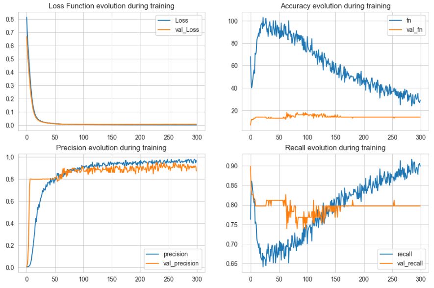
Let’s plot the keras.metrics vs Epochs
plt.figure(figsize=(12, 16))
plt.subplot(4, 2, 1)
plt.plot(r.history[‘loss’], label=’Loss’)
plt.plot(r.history[‘val_loss’], label=’val_Loss’)
plt.title(‘Loss Function evolution during training’)
plt.legend()
plt.subplot(4, 2, 2)
plt.plot(r.history[‘fn’], label=’fn’)
plt.plot(r.history[‘val_fn’], label=’val_fn’)
plt.title(‘Accuracy evolution during training’)
plt.legend()
plt.subplot(4, 2, 3)
plt.plot(r.history[‘precision’], label=’precision’)
plt.plot(r.history[‘val_precision’], label=’val_precision’)
plt.title(‘Precision evolution during training’)
plt.legend()
plt.subplot(4, 2, 4)
plt.plot(r.history[‘recall’], label=’recall’)
plt.plot(r.history[‘val_recall’], label=’val_recall’)
plt.title(‘Recall evolution during training’)
plt.legend()
plt.savefig(‘lossval.png’)
Given the above trained model, let’s predict labels of the train/test data
y_train_pred = model.predict(X_train)
y_test_pred = model.predict(X_test)
print_score(y_train, y_train_pred.round(), train=True)
print_score(y_test, y_test_pred.round(), train=False)
scores_dict = {
‘ANNs’: {
‘Train’: f1_score(y_train, y_train_pred.round()),
‘Test’: f1_score(y_test, y_test_pred.round()),
},
}
4985/4985 [==============================] - 4s 744us/step
2671/2671 [==============================] - 2s 783us/step
Train Result:
================================================
Accuracy Score: 99.99%
_______________________________________________
Classification Report:
                  0      1  accuracy  macro avg  weighted avg
precision      1.00   1.00      1.00       1.00          1.00
recall         1.00   0.97      1.00       0.98          1.00
f1-score       1.00   0.98      1.00       0.99          1.00
support   159204.00 287.00      1.00  159491.00     159491.00
_______________________________________________
Confusion Matrix:
 [[159203      1]
 [     9    278]]

Test Result:
================================================
Accuracy Score: 99.96%
_______________________________________________
Classification Report:
                 0      1  accuracy  macro avg  weighted avg
precision     1.00   0.90      1.00       0.95          1.00
recall        1.00   0.82      1.00       0.91          1.00
f1-score      1.00   0.86      1.00       0.93          1.00
support   85307.00 136.00      1.00   85443.00      85443.00
_______________________________________________
Confusion Matrix:
 [[85295    12]
 [   25   111]]
Multiple-Model Training & Validation
Let’s invoke several popular supervised ML binary classification algorithms.
XGBClassifier
from xgboost import XGBClassifier
xgb_clf = XGBClassifier()
xgb_clf.fit(X_train, y_train, eval_metric=’aucpr’)
y_train_pred = xgb_clf.predict(X_train)
y_test_pred = xgb_clf.predict(X_test)
print_score(y_train, y_train_pred, train=True)
print_score(y_test, y_test_pred, train=False)
scores_dict[‘XGBoost’] = {
‘Train’: f1_score(y_train,y_train_pred),
‘Test’: f1_score(y_test, y_test_pred),
}
Train Result:
================================================
Accuracy Score: 100.00%
_______________________________________________
Classification Report:
                  0      1  accuracy  macro avg  weighted avg
precision      1.00   1.00      1.00       1.00          1.00
recall         1.00   1.00      1.00       1.00          1.00
f1-score       1.00   1.00      1.00       1.00          1.00
support   159204.00 287.00      1.00  159491.00     159491.00
_______________________________________________
Confusion Matrix:
 [[159204      0]
 [     0    287]]

Test Result:
================================================
Accuracy Score: 99.96%
_______________________________________________
Classification Report:
                 0      1  accuracy  macro avg  weighted avg
precision     1.00   0.95      1.00       0.97          1.00
recall        1.00   0.82      1.00       0.91          1.00
f1-score      1.00   0.88      1.00       0.94          1.00
support   85307.00 136.00      1.00   85443.00      85443.00
_______________________________________________
Confusion Matrix:
 [[85301     6]
 [   25   111]]
RandomForestClassifier
from sklearn.ensemble import RandomForestClassifier
rf_clf = RandomForestClassifier(n_estimators=100, oob_score=False)
rf_clf.fit(X_train, y_train)
y_train_pred = rf_clf.predict(X_train)
y_test_pred = rf_clf.predict(X_test)
print_score(y_train, y_train_pred, train=True)
print_score(y_test, y_test_pred, train=False)
scores_dict[‘Random Forest’] = {
‘Train’: f1_score(y_train,y_train_pred),
‘Test’: f1_score(y_test, y_test_pred),
}
Train Result:
================================================
Accuracy Score: 100.00%
_______________________________________________
Classification Report:
                  0      1  accuracy  macro avg  weighted avg
precision      1.00   1.00      1.00       1.00          1.00
recall         1.00   1.00      1.00       1.00          1.00
f1-score       1.00   1.00      1.00       1.00          1.00
support   159204.00 287.00      1.00  159491.00     159491.00
_______________________________________________
Confusion Matrix:
 [[159204      0]
 [     0    287]]

Test Result:
================================================
Accuracy Score: 99.96%
_______________________________________________
Classification Report:
                 0      1  accuracy  macro avg  weighted avg
precision     1.00   0.90      1.00       0.95          1.00
recall        1.00   0.81      1.00       0.90          1.00
f1-score      1.00   0.85      1.00       0.93          1.00
support   85307.00 136.00      1.00   85443.00      85443.00
_______________________________________________
Confusion Matrix:
 [[85295    12]
 [   26   110]]
CatBoostClassifier
from catboost import CatBoostClassifier
cb_clf = CatBoostClassifier()
cb_clf.fit(X_train, y_train)
Learning rate set to 0.089847
0:	learn: 0.3914646	total: 169ms	remaining: 2m 49s
.....
999:	learn: 0.0001216	total: 16.6s	remaining: 0us
y_train_pred = cb_clf.predict(X_train)
y_test_pred = cb_clf.predict(X_test)
print_score(y_train, y_train_pred, train=True)
print_score(y_test, y_test_pred, train=False)
scores_dict[‘CatBoost’] = {
‘Train’: f1_score(y_train,y_train_pred),
‘Test’: f1_score(y_test, y_test_pred),
}
Train Result:
================================================
Accuracy Score: 100.00%
_______________________________________________
Classification Report:
                  0      1  accuracy  macro avg  weighted avg
precision      1.00   1.00      1.00       1.00          1.00
recall         1.00   1.00      1.00       1.00          1.00
f1-score       1.00   1.00      1.00       1.00          1.00
support   159204.00 287.00      1.00  159491.00     159491.00
_______________________________________________
Confusion Matrix:
 [[159204      0]
 [     1    286]]

Test Result:
================================================
Accuracy Score: 99.96%
_______________________________________________
Classification Report:
                 0      1  accuracy  macro avg  weighted avg
precision     1.00   0.93      1.00       0.97          1.00
recall        1.00   0.82      1.00       0.91          1.00
f1-score      1.00   0.87      1.00       0.94          1.00
support   85307.00 136.00      1.00   85443.00      85443.00
_______________________________________________
Confusion Matrix:
 [[85299     8]
 [   25   111]]
DecisionTreeClassifier
from sklearn.tree import DecisionTreeClassifier
lgbm_clf = DecisionTreeClassifier(random_state=0)
lgbm_clf.fit(X_train, y_train)
y_train_pred = lgbm_clf.predict(X_train)
y_test_pred = lgbm_clf.predict(X_test)
print_score(y_train, y_train_pred, train=True)
print_score(y_test, y_test_pred, train=False)
scores_dict[‘DTC’] = {
‘Train’: f1_score(y_train,y_train_pred),
‘Test’: f1_score(y_test, y_test_pred),
}
Train Result:
================================================
Accuracy Score: 100.00%
_______________________________________________
Classification Report:
                  0      1  accuracy  macro avg  weighted avg
precision      1.00   1.00      1.00       1.00          1.00
recall         1.00   1.00      1.00       1.00          1.00
f1-score       1.00   1.00      1.00       1.00          1.00
support   159204.00 287.00      1.00  159491.00     159491.00
_______________________________________________
Confusion Matrix:
 [[159204      0]
 [     0    287]]

Test Result:
================================================
Accuracy Score: 99.90%
_______________________________________________
Classification Report:
                 0      1  accuracy  macro avg  weighted avg
precision     1.00   0.66      1.00       0.83          1.00
recall        1.00   0.74      1.00       0.87          1.00
f1-score      1.00   0.69      1.00       0.85          1.00
support   85307.00 136.00      1.00   85443.00      85443.00
_______________________________________________
Confusion Matrix:
 [[85255    52]
 [   36   100]]
AdaBoostClassifier
from sklearn.ensemble import AdaBoostClassifier
lgbm_clf=AdaBoostClassifier()
lgbm_clf.fit(X_train, y_train)
y_train_pred = lgbm_clf.predict(X_train)
y_test_pred = lgbm_clf.predict(X_test)
print_score(y_train, y_train_pred, train=True)
print_score(y_test, y_test_pred, train=False)
scores_dict[‘Ada’] = {
‘Train’: f1_score(y_train,y_train_pred),
‘Test’: f1_score(y_test, y_test_pred),
}
Train Result:
================================================
Accuracy Score: 99.92%
_______________________________________________
Classification Report:
                  0      1  accuracy  macro avg  weighted avg
precision      1.00   0.80      1.00       0.90          1.00
recall         1.00   0.73      1.00       0.87          1.00
f1-score       1.00   0.76      1.00       0.88          1.00
support   159204.00 287.00      1.00  159491.00     159491.00
_______________________________________________
Confusion Matrix:
 [[159150     54]
 [    77    210]]

Test Result:
================================================
Accuracy Score: 99.93%
_______________________________________________
Classification Report:
                 0      1  accuracy  macro avg  weighted avg
precision     1.00   0.80      1.00       0.90          1.00
recall        1.00   0.76      1.00       0.88          1.00
f1-score      1.00   0.78      1.00       0.89          1.00
support   85307.00 136.00      1.00   85443.00      85443.00
_______________________________________________
Confusion Matrix:
 [[85281    26]
 [   32   104]]
GaussianNB
from sklearn.naive_bayes import GaussianNB
lgbm_clf=GaussianNB()
lgbm_clf.fit(X_train, y_train)
y_train_pred = lgbm_clf.predict(X_train)
y_test_pred = lgbm_clf.predict(X_test)
print_score(y_train, y_train_pred, train=True)
print_score(y_test, y_test_pred, train=False)
scores_dict[‘GNB’] = {
‘Train’: f1_score(y_train,y_train_pred),
‘Test’: f1_score(y_test, y_test_pred),
}
Train Result:
================================================
Accuracy Score: 97.77%
_______________________________________________
Classification Report:
                  0      1  accuracy  macro avg  weighted avg
precision      1.00   0.06      0.98       0.53          1.00
recall         0.98   0.82      0.98       0.90          0.98
f1-score       0.99   0.12      0.98       0.55          0.99
support   159204.00 287.00      0.98  159491.00     159491.00
_______________________________________________
Confusion Matrix:
 [[155706   3498]
 [    52    235]]

Test Result:
================================================
Accuracy Score: 97.78%
_______________________________________________
Classification Report:
                 0      1  accuracy  macro avg  weighted avg
precision     1.00   0.06      0.98       0.53          1.00
recall        0.98   0.85      0.98       0.92          0.98
f1-score      0.99   0.11      0.98       0.55          0.99
support   85307.00 136.00      0.98   85443.00      85443.00
_______________________________________________
Confusion Matrix:
 [[83428  1879]
 [   20   116]]
SVC
from sklearn.svm import SVC
lgbm_clf=SVC()
lgbm_clf.fit(X_train, y_train)
y_train_pred = lgbm_clf.predict(X_train)
y_test_pred = lgbm_clf.predict(X_test)
print_score(y_train, y_train_pred, train=True)
print_score(y_test, y_test_pred, train=False)
scores_dict[‘SVC’] = {
‘Train’: f1_score(y_train,y_train_pred),
‘Test’: f1_score(y_test, y_test_pred),
}
Train Result:
================================================
Accuracy Score: 99.96%
_______________________________________________
Classification Report:
                  0      1  accuracy  macro avg  weighted avg
precision      1.00   0.99      1.00       0.99          1.00
recall         1.00   0.81      1.00       0.91          1.00
f1-score       1.00   0.89      1.00       0.95          1.00
support   159204.00 287.00      1.00  159491.00     159491.00
_______________________________________________
Confusion Matrix:
 [[159201      3]
 [    54    233]]

Test Result:
================================================
Accuracy Score: 99.94%
_______________________________________________
Classification Report:
                 0      1  accuracy  macro avg  weighted avg
precision     1.00   0.92      1.00       0.96          1.00
recall        1.00   0.65      1.00       0.83          1.00
f1-score      1.00   0.76      1.00       0.88          1.00
support   85307.00 136.00      1.00   85443.00      85443.00
_______________________________________________
Confusion Matrix:
 [[85299     8]
 [   47    89]]
KNeighborsClassifier
from sklearn.neighbors import KNeighborsClassifier
lgbm_clf=KNeighborsClassifier()
lgbm_clf.fit(X_train, y_train)
y_train_pred = lgbm_clf.predict(X_train)
y_test_pred = lgbm_clf.predict(X_test)
print_score(y_train, y_train_pred, train=True)
print_score(y_test, y_test_pred, train=False)
scores_dict[‘KNN’] = {
‘Train’: f1_score(y_train,y_train_pred),
‘Test’: f1_score(y_test, y_test_pred),
}
Train Result:
================================================
Accuracy Score: 99.95%
_______________________________________________
Classification Report:
                  0      1  accuracy  macro avg  weighted avg
precision      1.00   0.96      1.00       0.98          1.00
recall         1.00   0.78      1.00       0.89          1.00
f1-score       1.00   0.86      1.00       0.93          1.00
support   159204.00 287.00      1.00  159491.00     159491.00
_______________________________________________
Confusion Matrix:
 [[159194     10]
 [    62    225]]

Test Result:
================================================
Accuracy Score: 99.94%
_______________________________________________
Classification Report:
                 0      1  accuracy  macro avg  weighted avg
precision     1.00   0.87      1.00       0.93          1.00
recall        1.00   0.77      1.00       0.89          1.00
f1-score      1.00   0.82      1.00       0.91          1.00
support   85307.00 136.00      1.00   85443.00      85443.00
_______________________________________________
Confusion Matrix:
 [[85291    16]
 [   31   105]]
LogisticRegression
from sklearn.linear_model import LogisticRegression
lgbm_clf=LogisticRegression()
lgbm_clf.fit(X_train, y_train)
y_train_pred = lgbm_clf.predict(X_train)
y_test_pred = lgbm_clf.predict(X_test)
print_score(y_train, y_train_pred, train=True)
print_score(y_test, y_test_pred, train=False)
scores_dict[‘LR’] = {
‘Train’: f1_score(y_train,y_train_pred),
‘Test’: f1_score(y_test, y_test_pred),
}
Train Result:
================================================
Accuracy Score: 99.92%
_______________________________________________
Classification Report:
                  0      1  accuracy  macro avg  weighted avg
precision      1.00   0.89      1.00       0.94          1.00
recall         1.00   0.62      1.00       0.81          1.00
f1-score       1.00   0.73      1.00       0.87          1.00
support   159204.00 287.00      1.00  159491.00     159491.00
_______________________________________________
Confusion Matrix:
 [[159182     22]
 [   108    179]]

Test Result:
================================================
Accuracy Score: 99.93%
_______________________________________________
Classification Report:
                 0      1  accuracy  macro avg  weighted avg
precision     1.00   0.87      1.00       0.93          1.00
recall        1.00   0.64      1.00       0.82          1.00
f1-score      1.00   0.74      1.00       0.87          1.00
support   85307.00 136.00      1.00   85443.00      85443.00
_______________________________________________
Confusion Matrix:
 [[85294    13]
 [   49    87]]
SGDClassifier
from sklearn.linear_model import SGDClassifier
lgbm_clf=SGDClassifier()
lgbm_clf.fit(X_train, y_train)
y_train_pred = lgbm_clf.predict(X_train)
y_test_pred = lgbm_clf.predict(X_test)
print_score(y_train, y_train_pred, train=True)
print_score(y_test, y_test_pred, train=False)
scores_dict[‘SGD’] = {
‘Train’: f1_score(y_train,y_train_pred),
‘Test’: f1_score(y_test, y_test_pred),
}
Train Result:
================================================
Accuracy Score: 99.91%
_______________________________________________
Classification Report:
                  0      1  accuracy  macro avg  weighted avg
precision      1.00   0.88      1.00       0.94          1.00
recall         1.00   0.58      1.00       0.79          1.00
f1-score       1.00   0.70      1.00       0.85          1.00
support   159204.00 287.00      1.00  159491.00     159491.00
_______________________________________________
Confusion Matrix:
 [[159182     22]
 [   121    166]]

Test Result:
================================================
Accuracy Score: 99.92%
_______________________________________________
Classification Report:
                 0      1  accuracy  macro avg  weighted avg
precision     1.00   0.85      1.00       0.92          1.00
recall        1.00   0.58      1.00       0.79          1.00
f1-score      1.00   0.69      1.00       0.84          1.00
support   85307.00 136.00      1.00   85443.00      85443.00
_______________________________________________
Confusion Matrix:
 [[85293    14]
 [   57    79]]
GradientBoostingClassifier
from sklearn.ensemble import GradientBoostingClassifier
lgbm_clf=GradientBoostingClassifier()
lgbm_clf.fit(X_train, y_train)
y_train_pred = lgbm_clf.predict(X_train)
y_test_pred = lgbm_clf.predict(X_test)
print_score(y_train, y_train_pred, train=True)
print_score(y_test, y_test_pred, train=False)
scores_dict[‘GBC’] = {
‘Train’: f1_score(y_train,y_train_pred),
‘Test’: f1_score(y_test, y_test_pred),
}
Train Result:
================================================
Accuracy Score: 99.85%
_______________________________________________
Classification Report:
                  0      1  accuracy  macro avg  weighted avg
precision      1.00   0.98      1.00       0.99          1.00
recall         1.00   0.19      1.00       0.59          1.00
f1-score       1.00   0.32      1.00       0.66          1.00
support   159204.00 287.00      1.00  159491.00     159491.00
_______________________________________________
Confusion Matrix:
 [[159203      1]
 [   233     54]]

Test Result:
================================================
Accuracy Score: 99.85%
_______________________________________________
Classification Report:
                 0      1  accuracy  macro avg  weighted avg
precision     1.00   0.73      1.00       0.86          1.00
recall        1.00   0.14      1.00       0.57          1.00
f1-score      1.00   0.23      1.00       0.62          1.00
support   85307.00 136.00      1.00   85443.00      85443.00
_______________________________________________
Confusion Matrix:
 [[85300     7]
 [  117    19]]
MLPClassifier
from sklearn.neural_network import MLPClassifier
lgbm_clf=MLPClassifier()
lgbm_clf.fit(X_train, y_train)
y_train_pred = lgbm_clf.predict(X_train)
y_test_pred = lgbm_clf.predict(X_test)
print_score(y_train, y_train_pred, train=True)
print_score(y_test, y_test_pred, train=False)
scores_dict[‘MLP’] = {
‘Train’: f1_score(y_train,y_train_pred),
‘Test’: f1_score(y_test, y_test_pred),
}
Train Result:
================================================
Accuracy Score: 99.98%
_______________________________________________
Classification Report:
                  0      1  accuracy  macro avg  weighted avg
precision      1.00   1.00      1.00       1.00          1.00
recall         1.00   0.87      1.00       0.93          1.00
f1-score       1.00   0.93      1.00       0.96          1.00
support   159204.00 287.00      1.00  159491.00     159491.00
_______________________________________________
Confusion Matrix:
 [[159203      1]
 [    38    249]]

Test Result:
================================================
Accuracy Score: 99.95%
_______________________________________________
Classification Report:
                 0      1  accuracy  macro avg  weighted avg
precision     1.00   0.92      1.00       0.96          1.00
recall        1.00   0.76      1.00       0.88          1.00
f1-score      1.00   0.83      1.00       0.92          1.00
support   85307.00 136.00      1.00   85443.00      85443.00
_______________________________________________
Confusion Matrix:
 [[85298     9]
 [   33   103]]
QuadraticDiscriminantAnalysis
from sklearn.discriminant_analysis import QuadraticDiscriminantAnalysis
lgbm_clf=QuadraticDiscriminantAnalysis()
lgbm_clf.fit(X_train, y_train)
y_train_pred = lgbm_clf.predict(X_train)
y_test_pred = lgbm_clf.predict(X_test)
print_score(y_train, y_train_pred, train=True)
print_score(y_test, y_test_pred, train=False)
scores_dict[‘QDA’] = {
‘Train’: f1_score(y_train,y_train_pred),
‘Test’: f1_score(y_test, y_test_pred),
}
Train Result:
================================================
Accuracy Score: 97.55%
_______________________________________________
Classification Report:
                  0      1  accuracy  macro avg  weighted avg
precision      1.00   0.06      0.98       0.53          1.00
recall         0.98   0.87      0.98       0.92          0.98
f1-score       0.99   0.11      0.98       0.55          0.99
support   159204.00 287.00      0.98  159491.00     159491.00
_______________________________________________
Confusion Matrix:
 [[155334   3870]
 [    38    249]]

Test Result:
================================================
Accuracy Score: 97.55%
_______________________________________________
Classification Report:
                 0      1  accuracy  macro avg  weighted avg
precision     1.00   0.06      0.98       0.53          1.00
recall        0.98   0.90      0.98       0.94          0.98
f1-score      0.99   0.11      0.98       0.55          0.99
support   85307.00 136.00      0.98   85443.00      85443.00
_______________________________________________
Confusion Matrix:
 [[83229  2078]
 [   13   123]]
Multiple-Model ML/DL F1-Score Comparison
scores_df = pd.DataFrame(scores_dict)
scores_df.plot(kind=’barh’, figsize=(15, 8),fontsize=16)

Best ML/DL Model Performance QC Analysis
Let’s compare ML/DL model results and performance using SciKit-Plot visualization
import scikitplot as skplt
import sklearn
from sklearn.model_selection import train_test_split
from sklearn.cluster import KMeans
from sklearn.decomposition import PCA
import matplotlib.pyplot as plt
import sys
import warnings
warnings.filterwarnings(“ignore”)
print(“Scikit Plot Version : “, skplt.version)
print(“Scikit Learn Version : “, sklearn.version)
print(“Python Version : “, sys.version)
%matplotlib inline
Scikit Plot Version :  0.3.7
Scikit Learn Version :  1.2.2
Python Version :  3.9.16 (main, Jan 11 2023, 16:16:36) [MSC v.1916 64 bit (AMD64)]
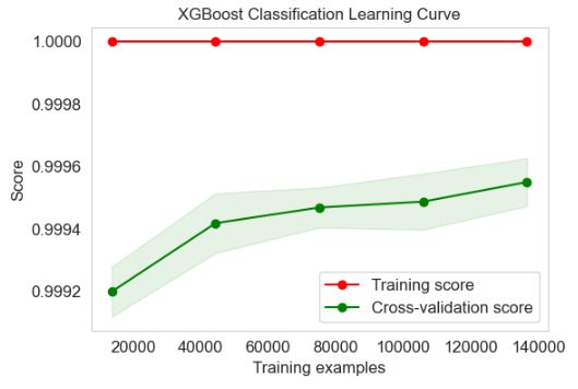
XGBoost Classification Learning Curve
skplt.estimators.plot_learning_curve(xgb_clf, X_train, y_train,
cv=7, shuffle=True, scoring=”accuracy”,
n_jobs=-1, figsize=(6,4), title_fontsize=”large”, text_fontsize=”large”,
title=”XGBoost Classification Learning Curve”);
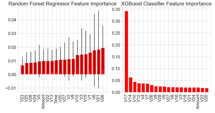
Feature Importance: Random Forest vs XGBoost Classifier
col=data.columns
col.drop(‘Class’)
Index(['Time', 'V1', 'V2', 'V3', 'V4', 'V5', 'V6', 'V7', 'V8', 'V9', 'V10',
       'V11', 'V12', 'V13', 'V14', 'V15', 'V16', 'V17', 'V18', 'V19', 'V20', 'V21', 'V22', 'V23', 'V24', 'V25', 'V26', 'V27', 'V28', 'Amount'],
      dtype='object')
fig = plt.figure(figsize=(11,6))
ax1 = fig.add_subplot(121)
skplt.estimators.plot_feature_importances(rf_clf, feature_names=col,
title=”Random Forest Regressor Feature Importance”,
x_tick_rotation=90, order=”ascending”,
ax=ax1);
ax2 = fig.add_subplot(122)
skplt.estimators.plot_feature_importances(xgb_clf, feature_names=col,
title=”XGBoost Classifier Feature Importance”,
x_tick_rotation=90,
ax=ax2);
plt.tight_layout()
Calibration Plots
lr_probas = CatBoostClassifier().fit(X_train, y_train).predict_proba(X_test)
rf_probas = RandomForestClassifier().fit(X_train, y_train).predict_proba(X_test)
gb_probas = XGBClassifier().fit(X_train, y_train).predict_proba(X_test)
et_scores = MLPClassifier().fit(X_train, y_train).predict_proba(X_test)
probas_list = [lr_probas, rf_probas, gb_probas, et_scores]
clf_names = [‘CatBoost’, ‘Random Forest’, ‘XGBoost’, ‘MLP’]
skplt.metrics.plot_calibration_curve(y_test,
probas_list,
clf_names, n_bins=15,
figsize=(12,6)
);
![Calibration plots clf_names = ['CatBoost', 'Random Forest', 'XGBoost', 'MLP']](https://newdigitals.org/wp-content/uploads/2023/05/credit_calibration_plots.jpg?w=913)
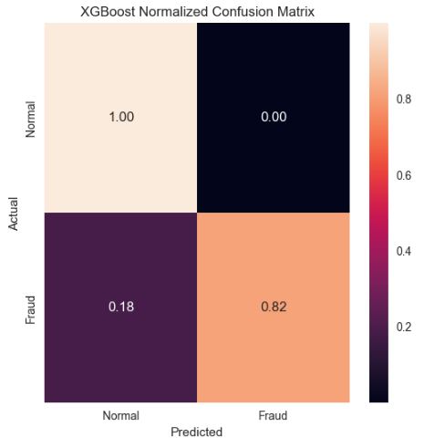
Normalized Confusion Matrix
y_train_pred = xgb_clf.predict(X_train)
y_test_pred = xgb_clf.predict(X_test)
target_names=[‘Normal’,’Fraud’]
from sklearn.metrics import confusion_matrix
import seaborn as sns
cm = confusion_matrix(y_test, y_test_pred)
cmn = cm.astype(‘float’) / cm.sum(axis=1)[:, np.newaxis]
fig, ax = plt.subplots(figsize=(6,6))
sns.heatmap(cmn, annot=True, fmt=’.2f’, xticklabels=target_names, yticklabels=target_names)
plt.ylabel(‘Actual’)
plt.xlabel(‘Predicted’)
plt.title(‘XGBoost Normalized Confusion Matrix’)
plt.show(block=True)
XGBoost ROC Curve
Y_test_probs = xgb_clf.predict_proba(X_test)
skplt.metrics.plot_roc_curve(y_test, Y_test_probs,
title=”XGBoost ROC Curve”, figsize=(12,6));

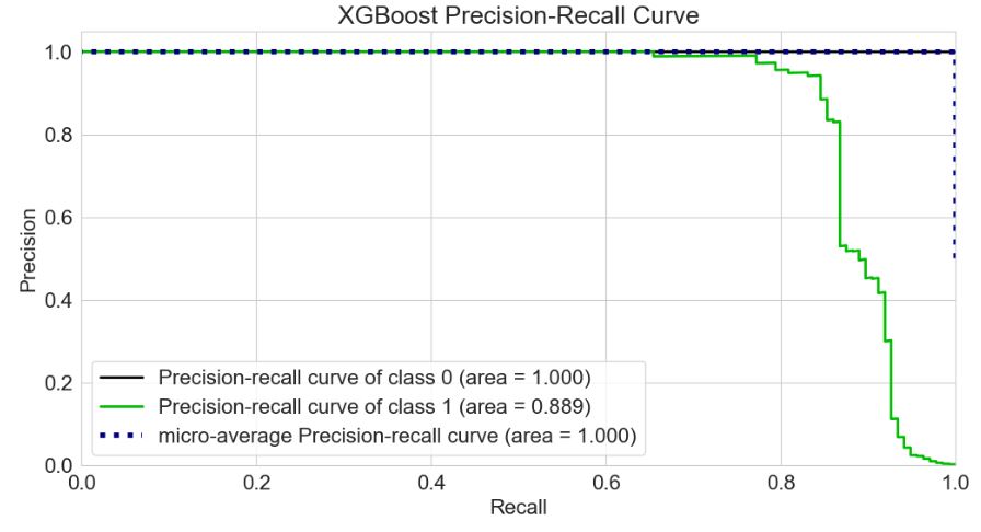
Precision-Recall Curve
skplt.metrics.plot_precision_recall_curve(y_test, Y_test_probs,
title=”XGBoost Precision-Recall Curve”, figsize=(12,6));
XGBoost KS Statistic Plot
Y_probas = xgb_clf.predict_proba(X_test)
skplt.metrics.plot_ks_statistic(y_test, Y_probas, figsize=(10,6));

XGBoost Cumulative Gains Curve
skplt.metrics.plot_cumulative_gain(y_test, Y_probas, figsize=(10,6));

XGBoost Lift Curve
skplt.metrics.plot_lift_curve(y_test, Y_probas, figsize=(10,6));

K-Means PCA Clusters & Variance Analysis
Elbow Plot
skplt.cluster.plot_elbow_curve(KMeans(random_state=1),
X_train,
cluster_ranges=range(2, 20),
figsize=(8,6));

Silhouette Analysis
kmeans = KMeans(n_clusters=10, random_state=1)
kmeans.fit(X_train, y_train)
cluster_labels = kmeans.predict(X_test)
skplt.metrics.plot_silhouette(X_test, cluster_labels,
figsize=(8,6));

PCA Component Explained Variances
pca = PCA(random_state=1)
pca.fit(X_train)
skplt.decomposition.plot_pca_component_variance(pca, figsize=(8,6));

PCA 2-D Projection
skplt.decomposition.plot_pca_2d_projection(pca, X_train, y_train,
figsize=(10,10),
cmap=”tab10″);

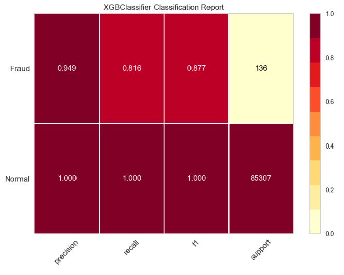
Final XGBoost Classification Report
from yellowbrick.classifier import ClassificationReport
viz = ClassificationReport(xgb_clf,
classes=target_names,
support=True,
fig=plt.figure(figsize=(8,6)))
viz.fit(X_train, y_train)
viz.score(X_test, y_test)
viz.show();
Summary of sklearn.metrics for XGBoost
from sklearn.metrics import class_likelihood_ratios
class_likelihood_ratios(y_test,y_test_pred)
(11604.261029411764, 0.18383645940293095)
from sklearn.metrics import balanced_accuracy_score
balanced_accuracy_score(y_test,y_test_pred)
0.9080530681917697
from sklearn.metrics import cohen_kappa_score
cohen_kappa_score(y_test,y_test_pred)
0.8772897054030634
from sklearn.metrics import hinge_loss
hinge_loss(y_test,y_test_pred)
0.9987711105649381
from sklearn.metrics import matthews_corrcoef
matthews_corrcoef(y_test,y_test_pred)
0.8797814646276692
from sklearn.metrics import roc_auc_score
roc_auc_score(y_test,y_test_pred)
0.9080530681917698
from sklearn.metrics import top_k_accuracy_score
top_k_accuracy_score(y_test,y_test_pred)
1.0
from sklearn.metrics import hamming_loss
hamming_loss(y_test,y_test_pred)
0.0003628149760659153
from sklearn.metrics import jaccard_score
jaccard_score(y_test,y_test_pred)
0.7816901408450704
from sklearn.metrics import log_loss
log_loss(y_test,y_test_pred)
0.013077177241700906
from sklearn.metrics import zero_one_loss
zero_one_loss(y_test,y_test_pred)
0.0003628149760659394
from sklearn.metrics import precision_recall_fscore_support
precision_recall_fscore_support(y_test,y_test_pred)
(array([0.99970701, 0.94871795]),
 array([0.99992967, 0.81617647]),
 array([0.99981832, 0.87747036]),
 array([85307,   136], dtype=int64))
from sklearn.metrics import f1_score
f1_score(y_test,y_test_pred)
0.8774703557312252
from sklearn.metrics import precision_score
precision_score(y_test,y_test_pred)
0.9487179487179487
from sklearn.metrics import recall_score
recall_score(y_test,y_test_pred)
0.8161764705882353
from sklearn.metrics import fbeta_score
fbeta_score(y_test,y_test_pred,beta=0.5)
0.9188741721854304
Discrimination Threshold
from yellowbrick.classifier import DiscriminationThreshold
viz = DiscriminationThreshold(xgb_clf,
classes=target_names,
cv=0.2,
fig=plt.figure(figsize=(9,6)))
viz.fit(X_train, y_train)
viz.score(X_test, y_test)
viz.show();

Summary
- This project presents a comparison of some established supervised ML and ANN algorithms to differentiate between genuine and fraudulent transactions.
- Multiple ML/DL models are built and fit on the training set, followed by comprehensive cross-validation and QC performance tests.
- We found that the XGBoost model performs the best in terms of FP = 18%, f1- and ROC-scores of 88% and 91%, respectively.
- Overfitting challenge: the model shows low bias but high variance. This is a result of an excessively complicated model, and it can be prevented by fitting multiple models and using validation or cross-validation to compare their predictive accuracies on test data.
- In principle, the obtained model can be applied in anti-fraud monitoring systems, or a similar CCFD model development process can be performed in related business areas to detect fraud.
Explore More


Make a one-time donation
Make a monthly donation
Make a yearly donation
Choose an amount
Or enter a custom amount
Your contribution is appreciated.
Your contribution is appreciated.
Your contribution is appreciated.
DonateDonate monthlyDonate yearly
Leave a comment