
Featured Photo by Element5 Digital on Pexels.
- Video games are an integral part of our lives. Expected to reach a value of $314bn by 2027, registering a CAGR of 9% over 2022-2027, gaming is set to become the new battleground for BigTech.
- Also, the number of new games released every year is increasing exponentially with 10,963 games released in 2022 alone.
- This has resulted in a large amount of data available that can be used to gain important BI insights.
- In this post, we will analyze video game sales and perform gaming industry market analysis in Python.
- This analysis will enable a game start-up firm launch a profitable product.
- The dataset contains a list of video games with sales greater than 100,000 copies. It was generated by a scrape of vgchartz.com. There are 16,598 records/rows and 11 attributes/columns
- Rank – Ranking based on overall sales
- Name – Name of the video game
- Platform – Platform on which the game is release
- Year – Year of the game’s release
- Genre – Genre of the game
- Publisher – Publisher of the game
- NA_Sales – Sales in North America (in millions)
- EU_Sales – Sales in Europe (in millions)
- JP_Sales – Sales in Japan (in millions)
- Other_Sales – Sales in the rest of the world (in millions)
- Global_Sales – Total worldwide sales.
- The script to scrape the data is available at https://github.com/GregorUT/vgchartzScrape.
- It is based on BeautifulSoup using Python.
Specific Questions:
- The game genre that generated the highest profit.
- Which Platforms have the highest sales price?
- Top Publishers and Total Revenue by Region
Import Modules
Let’s set the working directory
import os
os.chdir(‘VIDEOGAMES’)
os. getcwd()
and import the necessary modules/libraries
import pandas as pd
import numpy as np
import matplotlib.pyplot as plt
import seaborn as sns
%matplotlib inline
sns.set_style(‘darkgrid’)
Input Dataset
Let’s read the dataset
df = pd.read_csv(‘vgsales.csv’)
df.head()

Dataset shape
df.shape
(16598, 11)
Dataset type
df.dtypes
Rank              int64
Name             object
Platform         object
Year            float64
Genre            object
Publisher        object
NA_Sales        float64
EU_Sales        float64
JP_Sales        float64
Other_Sales     float64
Global_Sales    float64
dtype: object
Column names
df.columns
Index(['Rank', 'Name', 'Platform', 'Year', 'Genre', 'Publisher', 'NA_Sales',
       'EU_Sales', 'JP_Sales', 'Other_Sales', 'Global_Sales'],
      dtype='object')
Dataset summary
df.describe(include=’all’).T

Data Wrangling
Check for missing values
df.isnull().sum()
Rank              0
Name              0
Platform          0
Year            271
Genre             0
Publisher        58
NA_Sales          0
EU_Sales          0
JP_Sales          0
Other_Sales       0
Global_Sales      0
dtype: int64
Drop missing values
df = df.dropna()
(16291 rows × 11 columns)
Check if missing values have been removed
df.isnull().sum()
Rank            0
Name            0
Platform        0
Year            0
Genre           0
Publisher       0
NA_Sales        0
EU_Sales        0
JP_Sales        0
Other_Sales     0
Global_Sales    0
dtype: int64
Count number of entries in each column
df.count()
Rank            16291
Name            16291
Platform        16291
Year            16291
Genre           16291
Publisher       16291
NA_Sales        16291
EU_Sales        16291
JP_Sales        16291
Other_Sales     16291
Global_Sales    16291
dtype: int64
Check for duplicates
df.duplicated().any()
False
Convert year column from float to integers
df.Year = df.Year.astype(int)
Data Visualization Part 1
df_sum = df[df.columns.difference([‘Rank’,’Name’,’Platform’,’Genre’,’Publisher’])].sum()
df_sum
EU_Sales            2406.69
Global_Sales        8811.97
JP_Sales            1284.27
NA_Sales            4327.65
Other_Sales          788.91
Year            32686353.00
dtype: float64
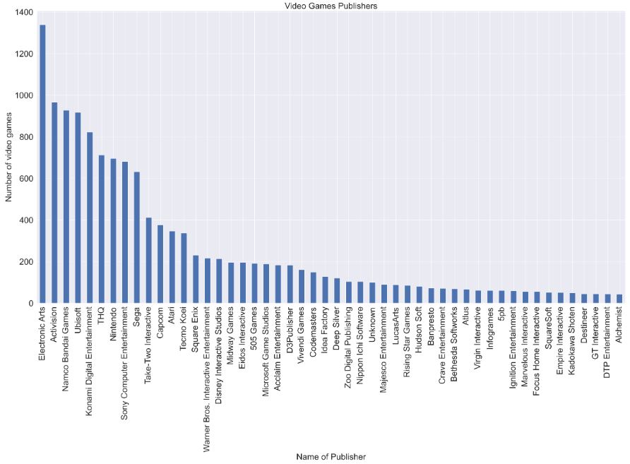
Let’s check the Number of video games vs Video Games Publishers
BIGGER_SIZE = 24
plt.rc(‘font’, size=BIGGER_SIZE) # controls default text sizes
plt.rc(‘axes’, titlesize=BIGGER_SIZE) # fontsize of the axes title
plt.rc(‘axes’, labelsize=BIGGER_SIZE) # fontsize of the x and y labels
plt.rc(‘xtick’, labelsize=BIGGER_SIZE) # fontsize of the tick labels
plt.rc(‘ytick’, labelsize=BIGGER_SIZE) # fontsize of the tick labels
plt.rc(‘legend’, fontsize=BIGGER_SIZE) # legend fontsize
plt.rc(‘figure’, titlesize=BIGGER_SIZE) # fontsize of the figure title
plt.figure(figsize=(30, 15))
df.Publisher.value_counts().nlargest(50).plot(kind=’bar’)
plt.title(‘Video Games Publishers’)
plt.xlabel(‘Name of Publisher’)
plt.ylabel(‘Number of video games’)
Let’s check video game genres
df.Genre.value_counts().nlargest(10).plot(kind=’bar’,figsize=(10,5))
plt.title(‘Video Game Genres’)
plt.xlabel(‘Genres’)
plt.ylabel(‘Number of video games’)
plt.savefig(‘numbergamesgenre.png’)

Let’s check the correlation between numeric columns in the dataset
plt.figure(figsize=(10,7))
v = df.corr()
sns.heatmap(v, cmap=’BrBG’,annot=True)

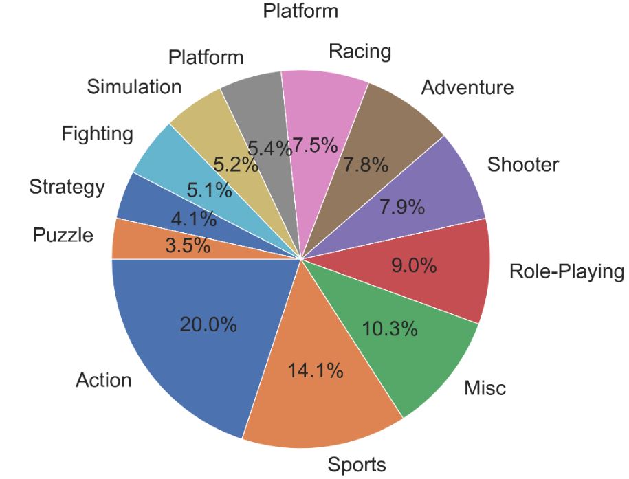
The Pie chart below is just the % distribution of Platforms in the Dataset
plt.figure(figsize=(20,10))
plt.title(‘Platform’)
plt.pie(df.Genre.value_counts(), labels=df.Genre.value_counts().index, autopct=’%1.1f%%’, startangle=180);
Let’s look at value_counts() of Publishers
df[‘Publisher’].value_counts()
Electronic Arts                 1339
Activision                       966
Namco Bandai Games               928
Ubisoft                          918
Konami Digital Entertainment     823
                                ...
Detn8 Games                        1
Pow                                1
Navarre Corp                       1
MediaQuest                         1
UIG Entertainment                  1
Name: Publisher, Length: 576, dtype: int64
Let’s check the total number of Platforms
df.Platform.nunique()
31
Let’s look at value_counts() of Genre
genre_counts = df.Genre.value_counts()
genre_counts
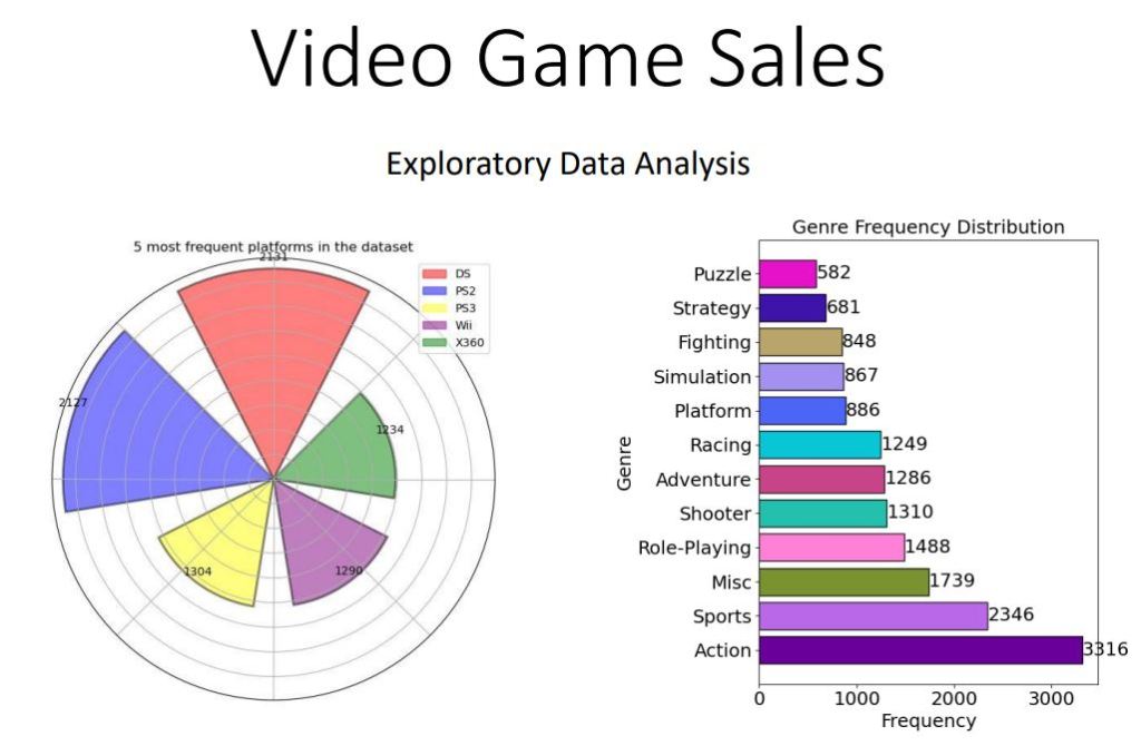
Action          3251
Sports          2304
Misc            1686
Role-Playing    1470
Shooter         1282
Adventure       1274
Racing          1225
Platform         875
Simulation       848
Fighting         836
Strategy         670
Puzzle           570
Name: Genre, dtype: int64
Let’s look at value_counts() of Platform
df[‘Platform’].value_counts()
DS      2131
PS2     2127
PS3     1304
Wii     1290
X360    1234
PSP     1197
PS      1189
PC       938
XB       803
GBA      786
GC       542
3DS      499
PSV      410
PS4      336
N64      316
SNES     239
XOne     213
SAT      173
WiiU     143
2600     116
NES       98
GB        97
DC        52
GEN       27
NG        12
SCD        6
WS         6
3DO        3
TG16       2
GG         1
PCFX       1
Name: Platform, dtype: int64
Data Visualization Part 2
Let’s look at the Video Games Sales dataset in data.world.
import warnings
warnings.filterwarnings(“ignore”)
import matplotlib.pyplot as plt
import seaborn as sns
sns.set()
%config InlineBackend.figure_format = ‘retina’
plt.rcParams[“figure.figsize”] = 8, 5
plt.rcParams[“image.cmap”] = “viridis”
import pandas as pd
df = pd.read_csv(“Video_Games.csv”).dropna()
print(df.shape)
(6825, 16)
Let’s edit the columns
df[“User_Score”] = df[“User_Score”].astype(“float64”)
df[“Year_of_Release”] = df[“Year_of_Release”].astype(“int64”)
df[“User_Count”] = df[“User_Count”].astype(“int64”)
df[“Critic_Count”] = df[“Critic_Count”].astype(“int64”)
useful_cols = [
“Name”,
“Platform”,
“Year_of_Release”,
“Genre”,
“Global_Sales”,
“Critic_Score”,
“Critic_Count”,
“User_Score”,
“User_Count”,
“Rating”,
]
df[useful_cols].head()

Let’s check top 5 platforms
top_platforms = (
df[“Platform”].value_counts().sort_values(ascending=False).head(5).index.values
)
sns.boxplot(
y=”Platform”,
x=”Critic_Score”,
data=df[df[“Platform”].isin(top_platforms)],
orient=”h”,
);

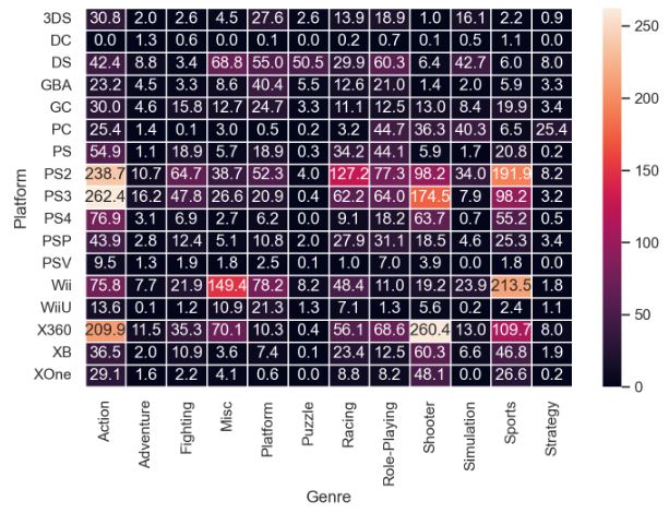
Let’s look at the pivot table Platform-Genre-Sales
platform_genre_sales = (
df.pivot_table(
index=”Platform”, columns=”Genre”, values=”Global_Sales”, aggfunc=sum
)
.fillna(0)
.applymap(float)
)
sns.heatmap(platform_genre_sales, annot=True, fmt=”.1f”, linewidths=0.5);
Let’s import plotly
import plotly
import plotly.graph_objs as go
from plotly.offline import download_plotlyjs, init_notebook_mode, iplot, plot
init_notebook_mode(connected=True)
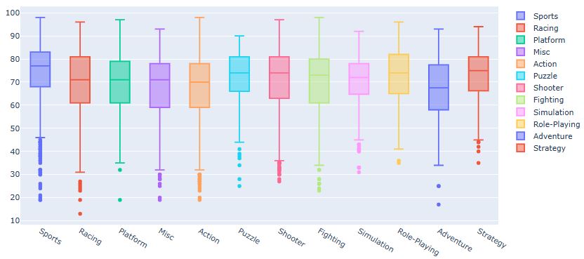
Let’s create a box trace of Critic_Score per genre in our dataset and visualize
data = []
for genre in df.Genre.unique():
data.append(go.Box(y=df[df.Genre == genre].Critic_Score, name=genre))
iplot(data, show_link=False)
Let’s look at the bar chart of genres vs total number of games released
rel = df.groupby([‘Genre’]).count().iloc[:,0]
rel = pd.DataFrame(rel.sort_values(ascending=False))
genres = rel.index
rel.columns = [‘Releases’]
colors = sns.color_palette(“summer”, len(rel))
plt.figure(figsize=(12,8))
ax = sns.barplot(y = genres , x = ‘Releases’, data=rel, orient=’h’, palette=colors)
ax.set_xlabel(xlabel=’Number of Releases’, fontsize=16)
ax.set_ylabel(ylabel=’Genre’, fontsize=16)
ax.set_title(label=’Genres by Total Number of Games Released’, fontsize=20)
ax.set_yticklabels(labels = genres, fontsize=14)
plt.show();

Let’s look at the bar chart of genres vs total revenue
rev = df.groupby([‘Genre’]).sum()[‘Global_Sales’]
rev = pd.DataFrame(rev.sort_values(ascending=False))
genres = rev.index
rev.columns = [‘Revenue’]
colors = sns.color_palette(‘Set3’, len(rev))
plt.figure(figsize=(12,8))
ax = sns.barplot(y = genres , x = ‘Revenue’, data=rev, orient=’h’, palette=colors)
ax.set_xlabel(xlabel=’Revenue in $ Millions’, fontsize=16)
ax.set_ylabel(ylabel=’Genre’, fontsize=16)
ax.set_title(label=’Genres by Total Revenue Generated in $ Millions’, fontsize=20)
ax.set_yticklabels(labels = genres, fontsize=14)
plt.show();

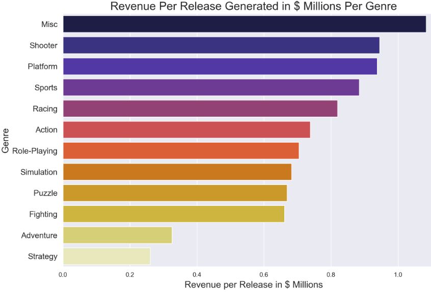
Let’s look at the bar chart revenue per release vs genre
data = pd.concat([rev, rel], axis=1)
data = pd.DataFrame(data[‘Revenue’] / data[‘Releases’])
data.columns = [‘Revenue Per Release’]
data = data.sort_values(by=’Revenue Per Release’,ascending=False)
genres = data.index
colors = sns.color_palette(“CMRmap”, len(data))
plt.figure(figsize=(12,8))
ax = sns.barplot(y = genres , x = ‘Revenue Per Release’, data=data, orient=’h’, palette=colors)
ax.set_xlabel(xlabel=’Revenue per Release in $ Millions’, fontsize=16)
ax.set_ylabel(ylabel=’Genre’, fontsize=16)
ax.set_title(label=’Revenue Per Release Generated in $ Millions Per Genre’, fontsize=20)
ax.set_yticklabels(labels = genres, fontsize=14)
plt.show();
Let’s look at the total revenue of top 10 games
data = pd.concat([df[‘Name’][0:10], df[‘Global_Sales’][0:10]], axis=1)
plt.figure(figsize=(12,8))
colors = sns.color_palette(“gist_earth”, len(data))
ax = sns.barplot(y = ‘Name’ , x = ‘Global_Sales’, data=data, orient=’h’, palette=colors)
ax.set_xlabel(xlabel=’Revenue in $ Millions’, fontsize=16)
ax.set_ylabel(ylabel=’Name’, fontsize=16)
ax.set_title(label=’Top 10 Games by Revenue Generated in $ Millions’, fontsize=20)
ax.set_yticklabels(labels = games, fontsize=14)
plt.show();

Data Visualization Part 3
Let’s look at the dataset vgsales.csv using plotly
import pandas as pd
import numpy as np
import plotly.express as px
import plotly.graph_objects as go
import plotly.figure_factory as ff
import plotly
import matplotlib.pyplot as plt
import re
from plotly.subplots import make_subplots
from scipy.stats import chi2_contingency
from wordcloud import wordcloud
df_train = pd.read_csv(‘vgsales.csv’)
df_train.info()
<class 'pandas.core.frame.DataFrame'>
RangeIndex: 16598 entries, 0 to 16597
Data columns (total 11 columns):
 #   Column        Non-Null Count  Dtype
---  ------        --------------  -----
 0   Rank          16598 non-null  int64
 1   Name          16598 non-null  object
 2   Platform      16598 non-null  object
 3   Year          16327 non-null  float64
 4   Genre         16598 non-null  object
 5   Publisher     16540 non-null  object
 6   NA_Sales      16598 non-null  float64
 7   EU_Sales      16598 non-null  float64
 8   JP_Sales      16598 non-null  float64
 9   Other_Sales   16598 non-null  float64
 10  Global_Sales  16598 non-null  float64
dtypes: float64(6), int64(1), object(4)
memory usage: 1.4+ MB
Let’s edit the data
df_train = df_train.dropna()
df_train = df_train.reset_index(drop = True)
df_train.loc[:, ‘Rank’] = np.arange(df_train.shape[0])+1
df_train[‘Year’] = df_train[‘Year’].astype(int)
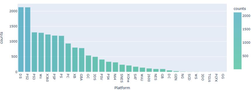
Let’s look at the platform counts
df_platcount = df_train.groupby(df_train[‘Platform’])[[‘Rank’]].count().rename(columns = {‘Rank’:’counts’}).sort_values(‘counts’, ascending = False)
fig = px.bar(df_platcount, x=df_platcount.index, y=’counts’, color=’counts’,color_continuous_scale=[‘rgba(17, 171, 122, 0.6)’, ‘rgba(17, 145, 171, 0.6)’],
height=400)
fig.show()
The following plotly bar chart is representative of the platforms linked to the top 100 games
df_platcount100 = df_train[0:100].groupby(df_train[‘Platform’])[[‘Rank’]].count().rename(columns = {‘Rank’:’counts’}).sort_values(‘counts’, ascending = False)
fig = px.bar(df_platcount100, x = df_platcount100.index, y = ‘counts’, color = ‘counts’, color_continuous_scale = [‘rgba(17, 171, 122. 0.6)’, ‘rgba(17, 145, 171, 0.6)’], height = 400)
fig.show()

Let’s check the Publisher rank counts
df_pubcount = df_train.groupby(df_train[‘Publisher’])[[‘Rank’]].count().rename(columns = {‘Rank’:’counts’}).sort_values(‘counts’, ascending = False)[:10]
fig = px.bar(df_pubcount, x = df_pubcount.index, y=’counts’, color=’counts’,color_continuous_scale=[‘rgb(17, 171, 122, 0.6)’, ‘rgb(17, 145, 171, 0.6)’],
height=400)
fig.show()

Let’s plot the plotly pie chart of Publisher vs Rank counts for the top 100 games
df_pubcount100 = df_train[:100].groupby(df_train[‘Publisher’])[[‘Rank’]].count().rename(columns = {‘Rank’:’counts’}).sort_values(‘counts’, ascending = False)
fig = px.pie(df_pubcount100 , names=df_pubcount100.index, values=’counts’, template=’seaborn’)
fig.update_traces(pull=[0.06,0.06,0.06,0.06,0.06], textinfo=”percent+label”)
fig.show()

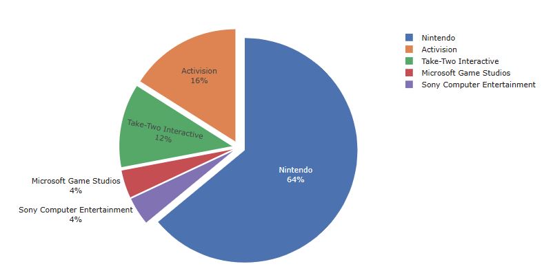
Let’s plot the plotly pie chart of Publisher vs Rank counts for the top 50 games
df_pubcount100 = df_train[:50].groupby(df_train[‘Publisher’])[[‘Rank’]].count().rename(columns = {‘Rank’:’counts’}).sort_values(‘counts’, ascending = False)
fig = px.pie(df_pubcount100 , names=df_pubcount100.index, values =’counts’, template=’seaborn’)
fig.update_traces(pull=[0.06,0.06,0.06,0.06,0.06], textinfo=”percent+label”)
fig.show()
Let’s examine the treemap Genre vs Rank and Sales
df_genrecount = df_train.groupby(df_train[‘Genre’])[[‘Rank’]].count().rename(columns = {‘Rank’:’counts’}).sort_values(‘counts’, ascending = False)
df_genresales = df_train.groupby(df_train[‘Genre’])[[‘Global_Sales’]].sum().sort_values(‘Global_Sales’, ascending = False)
fig = px.treemap(
names = df_genrecount.index, parents = [‘total’]*12,
values = df_genrecount[‘counts’],color=df_genresales[‘Global_Sales’],
color_continuous_scale=’jet’,
color_continuous_midpoint=np.average(df_genresales[‘Global_Sales’])
)
fig.show()

Let’s examine the treemap Genre vs Rank and Sales for the top 100 games
df_genrecount100 = df_train[0:100].groupby(df_train[‘Genre’])[[‘Rank’]].count().rename(columns = {‘Rank’:’counts’}).sort_values(‘counts’, ascending = False)
df_genresales100 = df_train[0:100].groupby(df_train[‘Genre’])[[‘Global_Sales’]].sum().sort_values(‘Global_Sales’, ascending = False)
fig = px.treemap(
names = df_genrecount100.index, parents = [‘total’]*11,
values = df_genrecount100[‘counts’],color=df_genresales100[‘Global_Sales’],
color_continuous_scale=’jet’,
color_continuous_midpoint=np.average(df_genresales100[‘Global_Sales’])
)
fig.show()

Let’s plot the treemap Genre vs Rank and Sales for the top 10 games
df_genrecount10 = df_train[0:10].groupby(df_train[‘Genre’])[[‘Rank’]].count().rename(columns = {‘Rank’:’counts’}).sort_values(‘counts’, ascending = False)
df_genresales10 = df_train[0:10].groupby(df_train[‘Genre’])[[‘Global_Sales’]].sum().sort_values(‘Global_Sales’, ascending = False)
fig = px.treemap(
names = df_genrecount10. index, parents = [‘total’]*7,
values = df_genrecount10[‘counts’],color=df_genresales10[‘Global_Sales’],
color_continuous_scale=’jet’,
color_continuous_midpoint=np.average(df_genresales10[‘Global_Sales’])
)
fig.show()

Let’s compare game sales per region
region_sec = df_train[[‘NA_Sales’, ‘EU_Sales’, ‘JP_Sales’, ‘Other_Sales’]].apply(lambda x: x. sum (), axis = 0)
region_sum = pd.DataFrame.from_dict(region_sec.to_dict(), orient = ‘index’, columns = [‘sum’]).sort_values(‘sum’, ascending = False)
fig = px.pie(region_sum , names=region_sum.index, values=’sum’, template=’seaborn’)
fig.update_traces(pull=[0,0.01,0.01,0.01],textinfo=”percent+label”)
fig.show()

Let’s check regional sales per genre
genre = df_train[‘Genre’].unique()
genre_s = sorted(genre)
na_sales=[]
eu_sales=[]
jp_sales=[]
other_sales=[]
global_sales=[]
for i in genre_s:
val= df_train[df_train.Genre==i]
na_sales.append(val.NA_Sales.sum())
eu_sales.append(val.EU_Sales.sum())
jp_sales.append(val.JP_Sales.sum())
other_sales.append(val.Other_Sales.sum())
fig = go.Figure()
fig.add_trace(go.Bar(x=na_sales,
y=genre_s,
name=’North America Sales’,
marker_color=’teal’,
orientation=’h’))
fig.add_trace(go.Bar(x=eu_sales,
y=genre_s,
name=’Europe Sales’,
marker_color=’purple’,
orientation=’h’))
fig.add_trace(go.Bar(x=jp_sales,
y=genre_s,
name=’Japan Sales’,
marker_color=’gold’,
orientation=’h’))
fig.add_trace(go.Bar(x=other_sales,
y=genre_s,
name=’Other Region Sales’,
marker_color=’deepskyblue’,
orientation=’h’))
fig.update_layout(title_text=’Regional Sales by Genre’,xaxis_title=”Sales in $M”,yaxis_title=”Genre”,
barmode=’stack’)
fig.show()

Data Visualization Part 4
Let’s continue our analysis of the dataset vgsales.csv by comparing sns plots
import numpy as np
import pandas as pd
import scipy.stats as st
pd.set_option(‘display.max_columns’, None)
import math
import matplotlib.pyplot as plt
%matplotlib inline
import seaborn as sns
sns.set_style(‘whitegrid’)
import missingno as msno
from sklearn.preprocessing import StandardScaler
from scipy import stats
data = pd.read_csv(‘vgsales.csv’)
data.head()
drop_row_index = data[data[‘Year’] > 2015].index
data = data.drop(drop_row_index)
data.shape
(16250, 11)
data.isnull().sum()
Rank              0
Name              0
Platform          0
Year            271
Genre             0
Publisher        56
NA_Sales          0
EU_Sales          0
JP_Sales          0
Other_Sales       0
Global_Sales      0
dtype: int64
Let’s count Genre
data[‘Genre’].value_counts()
Action          3196
Sports          2308
Misc            1721
Role-Playing    1446
Shooter         1278
Adventure       1252
Racing          1229
Platform         876
Simulation       857
Fighting         834
Strategy         671
Puzzle           582
Name: Genre, dtype: int64
Let’s look at the sns countplot of Genre
BIGGER_SIZE = 18
plt.rc(‘font’, size=BIGGER_SIZE) # controls default text sizes
plt.rc(‘axes’, titlesize=BIGGER_SIZE) # fontsize of the axes title
plt.rc(‘axes’, labelsize=BIGGER_SIZE) # fontsize of the x and y labels
plt.rc(‘xtick’, labelsize=BIGGER_SIZE) # fontsize of the tick labels
plt.rc(‘ytick’, labelsize=BIGGER_SIZE) # fontsize of the tick labels
plt.rc(‘legend’, fontsize=BIGGER_SIZE) # legend fontsize
plt.rc(‘figure’, titlesize=BIGGER_SIZE) # fontsize of the figure title
plt.figure(figsize=(15, 10))
sns.countplot(x=”Genre”, data=data, order = data[‘Genre’].value_counts().index)
plt.xticks(rotation=90)
(array([ 0,  1,  2,  3,  4,  5,  6,  7,  8,  9, 10, 11]),
 [Text(0, 0, 'Action'),
  Text(1, 0, 'Sports'),
  Text(2, 0, 'Misc'),
  Text(3, 0, 'Role-Playing'),
  Text(4, 0, 'Shooter'),
  Text(5, 0, 'Adventure'),
  Text(6, 0, 'Racing'),
  Text(7, 0, 'Platform'),
  Text(8, 0, 'Simulation'),
  Text(9, 0, 'Fighting'),
  Text(10, 0, 'Strategy'),
  Text(11, 0, 'Puzzle')])

Let’s check the sns barplot of Sales vs Genre
data_genre = data.groupby(by=[‘Genre’])[‘Global_Sales’].sum()
data_genre = data_genre.reset_index()
data_genre = data_genre.sort_values(by=[‘Global_Sales’], ascending=False)
plt.figure(figsize=(15, 10))
sns.barplot(x=”Genre”, y=”Global_Sales”, data=data_genre)
plt.xticks(rotation=90)

Let’s check the sns barplot of Sales vs Platform
data_platform = data.groupby(by=[‘Platform’])[‘Global_Sales’].sum()
data_platform = data_platform.reset_index()
data_platform = data_platform.sort_values(by=[‘Global_Sales’], ascending=False)
plt.figure(figsize=(15, 10))
sns.barplot(x=”Platform”, y=”Global_Sales”, data=data_platform)
plt.xticks(rotation=90)

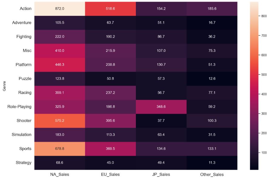
Let’s plot the sns heatmap Genre vs Region
comp_genre = data[[‘Genre’, ‘NA_Sales’, ‘EU_Sales’, ‘JP_Sales’, ‘Other_Sales’]]
comp_map = comp_genre.groupby(by=[‘Genre’]).sum()
plt.figure(figsize=(15, 10))
sns.set(font_scale=1)
sns.heatmap(comp_map, annot=True, fmt = ‘.1f’)
plt.xticks(fontsize=14)
plt.yticks(fontsize=14)
plt.show()
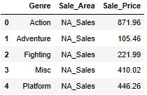
Let’s create the following table
comp_table = comp_map.reset_index()
comp_table = pd.melt(comp_table, id_vars=[‘Genre’], value_vars=[‘NA_Sales’, ‘EU_Sales’, ‘JP_Sales’, ‘Other_Sales’], var_name=’Sale_Area’, value_name=’Sale_Price’)
comp_table.head()
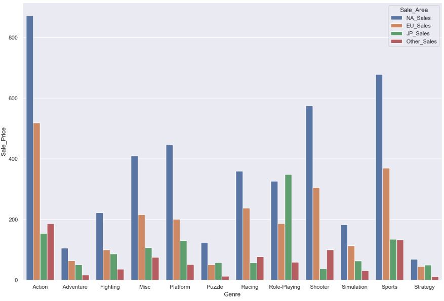
and plot x=’Genre’, y=’Sale_Price’, hue=’Sale_Area’
plt.figure(figsize=(15, 10))
sns.barplot(x=’Genre’, y=’Sale_Price’, hue=’Sale_Area’, data=comp_table)
Let’s create the following table
comp_platform = data[[‘Platform’, ‘NA_Sales’, ‘EU_Sales’, ‘JP_Sales’, ‘Other_Sales’]]
comp_platform.head()

Let’s look at sns.barplot with x=’Platform’, y=’Sale_Price’, hue=’Sale_Area’
BIGGER_SIZE = 24
plt.rc(‘font’, size=BIGGER_SIZE) # controls default text sizes
plt.rc(‘axes’, titlesize=BIGGER_SIZE) # fontsize of the axes title
plt.rc(‘axes’, labelsize=BIGGER_SIZE) # fontsize of the x and y labels
plt.rc(‘xtick’, labelsize=BIGGER_SIZE) # fontsize of the tick labels
plt.rc(‘ytick’, labelsize=BIGGER_SIZE) # fontsize of the tick labels
plt.rc(‘legend’, fontsize=BIGGER_SIZE) # legend fontsize
plt.rc(‘figure’, titlesize=BIGGER_SIZE) # fontsize of the figure title
plt.figure(figsize=(30, 15))
sns.barplot(x=’Platform’, y=’Sale_Price’, hue=’Sale_Area’, data=comp_table)
plt.xticks(fontsize=14)
plt.yticks(fontsize=14)
plt.show()

Let’s look at top 20 publishers
top_publisher = data.groupby(by=[‘Publisher’])[‘Year’].count().sort_values(ascending=False).head(20)
top_publisher = pd.DataFrame(top_publisher).reset_index()
BIGGER_SIZE = 18
plt.rc(‘font’, size=BIGGER_SIZE) # controls default text sizes
plt.rc(‘axes’, titlesize=BIGGER_SIZE) # fontsize of the axes title
plt.rc(‘axes’, labelsize=BIGGER_SIZE) # fontsize of the x and y labels
plt.rc(‘xtick’, labelsize=BIGGER_SIZE) # fontsize of the tick labels
plt.rc(‘ytick’, labelsize=BIGGER_SIZE) # fontsize of the tick labels
plt.rc(‘legend’, fontsize=BIGGER_SIZE) # legend fontsize
plt.rc(‘figure’, titlesize=BIGGER_SIZE) # fontsize of the figure title
plt.figure(figsize=(15, 10))
sns.countplot(x=”Publisher”, data=data, order = data.groupby(by=[‘Publisher’])[‘Year’].count().sort_values(ascending=False).iloc[:20].index)
plt.xticks(rotation=90)

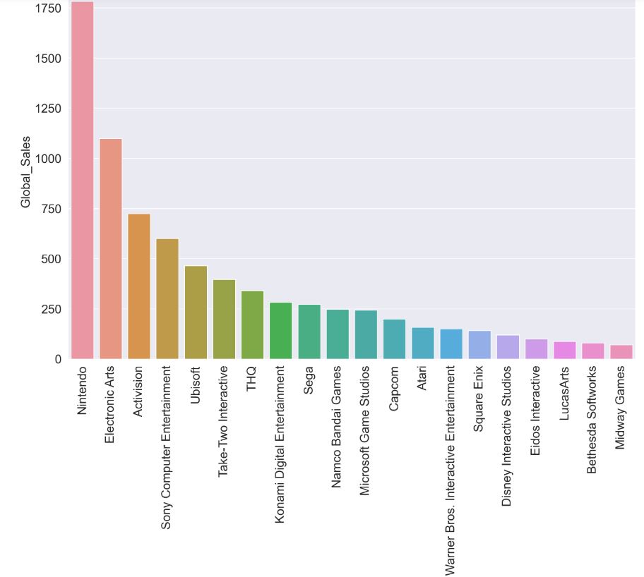
Let’s create the sns barplot x=’Publisher’, y=’Global_Sales’
sale_pbl = data[[‘Publisher’, ‘Global_Sales’]]
sale_pbl = sale_pbl.groupby(‘Publisher’)[‘Global_Sales’].sum().sort_values(ascending=False).head(20)
sale_pbl = pd.DataFrame(sale_pbl).reset_index()
plt.figure(figsize=(15, 10))
sns.barplot(x=’Publisher’, y=’Global_Sales’, data=sale_pbl)
plt.xticks(rotation=90)
Let’s plot sns.barplot with x=’Publisher’, y=’Sale_Price’, hue=’Sale_Area’ for top 20 Publishers
comp_publisher = data[[‘Publisher’, ‘NA_Sales’, ‘EU_Sales’, ‘JP_Sales’, ‘Other_Sales’, ‘Global_Sales’]]
comp_publisher.head()
comp_publisher = comp_publisher.groupby(by=[‘Publisher’]).sum().reset_index().sort_values(by=[‘Global_Sales’], ascending=False)
comp_publisher = comp_publisher.head(20)
comp_publisher = pd.melt(comp_publisher, id_vars=[‘Publisher’], value_vars=[‘NA_Sales’, ‘EU_Sales’, ‘JP_Sales’, ‘Other_Sales’], var_name=’Sale_Area’, value_name=’Sale_Price’)
comp_publisher
BIGGER_SIZE = 24
plt.rc(‘font’, size=BIGGER_SIZE) # controls default text sizes
plt.rc(‘axes’, titlesize=BIGGER_SIZE) # fontsize of the axes title
plt.rc(‘axes’, labelsize=BIGGER_SIZE) # fontsize of the x and y labels
plt.rc(‘xtick’, labelsize=BIGGER_SIZE) # fontsize of the tick labels
plt.rc(‘ytick’, labelsize=BIGGER_SIZE) # fontsize of the tick labels
plt.rc(‘legend’, fontsize=BIGGER_SIZE) # legend fontsize
plt.rc(‘figure’, titlesize=BIGGER_SIZE) # fontsize of the figure title
plt.figure(figsize=(20, 10))
sns.barplot(x=’Publisher’, y=’Sale_Price’, hue=’Sale_Area’, data=comp_publisher)
plt.xticks(fontsize=14, rotation=90)
plt.yticks(fontsize=14)
plt.show()

Let’s create the table
top_sale_reg = data[[‘NA_Sales’, ‘EU_Sales’, ‘JP_Sales’, ‘Other_Sales’]]
top_sale_reg = top_sale_reg.sum().reset_index()
top_sale_reg = top_sale_reg.rename(columns={“index”: “region”, 0: “sale”})
top_sale_reg

and get the sns barplot region vs sale
plt.figure(figsize=(12, 8))
sns.barplot(x=’region’, y=’sale’, data = top_sale_reg)

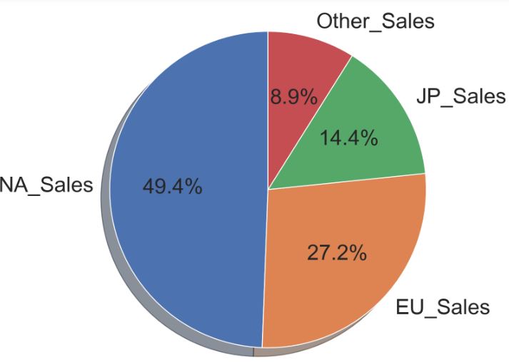
Let’s look at the % region vs sale as plt pie chart
labels = top_sale_reg[‘region’]
sizes = top_sale_reg[‘sale’]
plt.figure(figsize=(10, 8))
plt.pie(sizes, labels=labels, autopct=’%1.1f%%’, shadow=True, startangle=90)
Let’s compute the data correlation matrix
plt.figure(figsize=(13,10))
sns.heatmap(data.corr(), cmap = “Blues”, annot=True, linewidth=3)

Subsector Analysis
- The gaming industry roughly splits into 3 main subgroups: console, PC, and smartphone.
- The console subsector is the oldest and most consolidated with the largest global players being Nintendo, Sony, and Microsoft.
- Japanese Nintendo targets casual gamers between the ages of 15-30 and has been consistently outselling Xbox and PS5 for the past two years.
- In its PS5 launch, Sony confirmed that users will only be able to play on Sony’s console.
- The PC’s subsector, emerged later in time, and as opposed to the console industry is highly fragmented. Companies offer products like keyboards, advanced PC components and monitors to support gaming.
- Smartphone gaming is the newest sector within the industry, recording $79bn in revenues in 2021, and is also the most profitable subsector.
US Outlook 2023
- In 2022, we estimated that more than half (54.2%) of the US population were digital gamers.
- 2023 could be a banner year for the gaming industry, with advancing technology supercharging game product sales.
- A combination of AI and virtual reality (VR) innovations have improved the gaming experience significantly. The use of AI are giving rise to enhanced artistic qualities and photorealistic animation, as well as originality in dialogue and character depth.
- As companies invest in AI and VR, and even 5G infrastructure, expect more impressive-looking games to drive adoption, especially among Gen Z.
- Microsoft’s attempt to acquire Activision Blizzard. The $68.7 billion acquisition would give Microsoft a leadership position.
- Other major media powerhouses such as Netflix are investing in the gaming industry, too. Netflix is adding two more games (Kentucky Route Zero and Twelve Minutes) to its platform, bringing the total number of games available on the service to 48.
Inferences
- Most Popular Genre: Action.
- Action and Sport have highest sales.
- North America have highest sales for every genre.
- Best choice of Platform: DS offers the highest number of games with a total of 2131.
- Highest global sales is PS2. Console launched in 2000 and yet still the unbeaten compared to the rest and even to its upgrade PS3.
- Best choice of Publisher: Electronic Arts sold the highest number of unique games with a frequency of 1364.
- Highest correlations between NA/EU and Global Sales.

Source: adityavipradas
Sources
- Explore Video Game Sales Data
- Video Game Sales EDA, Visualizations, ML Models
- Bilal Data Wrangling and EDA Video Games Sales
- Video Games Sales Analysis
- EXPLORATORY DATA ANALYSIS ON VIDEO GAMES SALES
- Video Games Sales
- World Economic Forum
- BSIC
- Insider Intelligence
- Market Research
Infographic


Make a one-time donation
Make a monthly donation
Make a yearly donation
Choose an amount
Or enter a custom amount
Your contribution is appreciated.
Your contribution is appreciated.
Your contribution is appreciated.
DonateDonate monthlyDonate yearly
Leave a comment