JPM Breakouts: Auto ARIMA, FFT, LSTM & Stock Indicators

Featured Photo by Pixabay

In this post, we will look at the JPM stock price and relevant breakout strategies for 2022-23. Referring to the previous case study, our goal is to combine the Auto ARIMA, FFT, LSTM models and Technical Trading Indicators (TTIs) into a single framework to optimize advantages of each. Specifically, we will focus on the following TTIs: EMA, RSI, OBV, and MCAD.

Table of Contents

1. ARIMA
2. FFT
3. TTIs
4. LSTM
5. Summary
6. Continue Reading
7. Algo Trading Links
8. Stock Market Links
9. min(Risk/Reward Ratio) Links
10. Portfolio De-Risking Links

ARIMA

Let’s set the working directory

import os
os.chdir(‘YOURPATH’)
os. getcwd()

Let’s download the input data

import yfinance as yf
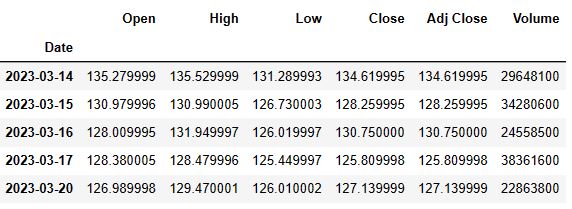
gs = yf.download(“JPM”, start=”2022-01-03″, end=”2023-03-21″)

[*********************100%***********************]  1 of 1 completed

gs.tail()

Let’s preprocess the data

import pandas as pd

dataset_ex_df = gs.copy()
dataset_ex_df = dataset_ex_df.reset_index()
dataset_ex_df[‘Date’] = pd.to_datetime(dataset_ex_df[‘Date’])
dataset_ex_df.set_index(‘Date’, inplace=True)
dataset_ex_df = dataset_ex_df[‘Close’].to_frame()

Let’s run Auto ARIMA to select optimal ARIMA parameters

from pmdarima.arima import auto_arima

model = auto_arima(dataset_ex_df[‘Close’], seasonal=False, trace=True)
print(model.summary())

Performing stepwise search to minimize aic
 ARIMA(2,1,2)(0,0,0)[0] intercept   : AIC=inf, Time=0.32 sec
 ARIMA(0,1,0)(0,0,0)[0] intercept   : AIC=1393.617, Time=0.01 sec
 ARIMA(1,1,0)(0,0,0)[0] intercept   : AIC=1394.786, Time=0.02 sec
 ARIMA(0,1,1)(0,0,0)[0] intercept   : AIC=1394.835, Time=0.02 sec
 ARIMA(0,1,0)(0,0,0)[0]             : AIC=1392.302, Time=0.01 sec
 ARIMA(1,1,1)(0,0,0)[0] intercept   : AIC=1396.288, Time=0.07 sec

Best model:  ARIMA(0,1,0)(0,0,0)[0]          
Total fit time: 0.456 seconds
                               SARIMAX Results                                
==============================================================================
Dep. Variable:                      y   No. Observations:                  304
Model:               SARIMAX(0, 1, 0)   Log Likelihood                -695.151
Date:                Tue, 21 Mar 2023   AIC                           1392.302
Time:                        11:09:24   BIC                           1396.016
Sample:                             0   HQIC                          1393.788
                                - 304                                         
Covariance Type:                  opg                                         
==============================================================================
                 coef    std err          z      P>|z|      [0.025      0.975]
------------------------------------------------------------------------------
sigma2         5.7579      0.365     15.773      0.000       5.042       6.473
===================================================================================
Ljung-Box (L1) (Q):                   0.82   Jarque-Bera (JB):                22.57
Prob(Q):                              0.36   Prob(JB):                         0.00
Heteroskedasticity (H):               0.50   Skew:                            -0.25
Prob(H) (two-sided):                  0.00   Kurtosis:                         4.24
===================================================================================

Warnings:
[1] Covariance matrix calculated using the outer product of gradients (complex-step).

Let’s define the ARIMA prediction model

from statsmodels.tsa.arima.model import ARIMA
import numpy as np

def arima_forecast(history):
# Fit the model
model = ARIMA(history, order=(0,1,0))
model_fit = model.fit()

# Make the prediction
output = model_fit.forecast()
yhat = output[0]
return yhat

Let’s split the data into train and test sets
X = dataset_ex_df.values
size = int(len(X) * 0.8)
train, test = X[0:size], X[size:len(X)]

Walk-forward validation to generate a prediction:
history = [x for x in train]
predictions = list()
for t in range(len(test)):
yhat = arima_forecast(history)
predictions.append(yhat)
Let’s add the predicted value to the training set
obs = test[t]
history.append(obs)

Let’s plot the result

import matplotlib.pyplot as plt

plt.figure(figsize=(12, 6), dpi=100)
plt.plot(dataset_ex_df.iloc[size:,:].index, test, label=’Real’)
plt.plot(dataset_ex_df.iloc[size:,:].index, predictions, color=’red’, label=’Predicted’)
plt.title(‘ARIMA Predictions vs Actual Values’)
plt.xlabel(‘Date’)
plt.ylabel(‘Stock Price’)
plt.legend()
plt.show()

FFT

Let’ calculate the Fourier Transform
data_FT = dataset_ex_df[[‘Close’]]
close_fft = np.fft.fft(np.asarray(data_FT[‘Close’].tolist()))
fft_df = pd.DataFrame({‘fft’:close_fft})
fft_df[‘absolute’] = fft_df[‘fft’].apply(lambda x: np.abs(x))
fft_df[‘angle’] = fft_df[‘fft’].apply(lambda x: np.angle(x))

and plot the partial Fourier Transforms
plt.figure(figsize=(14, 7), dpi=100)
plt.plot(np.asarray(data_FT[‘Close’].tolist()), label=’Real’)
for num_ in [9, 12, 15]:
fft_list_m10= np.copy(close_fft); fft_list_m10[num_:-num_]=0
plt.plot(np.fft.ifft(fft_list_m10), label=’Fourier transform with {} components’.format(num_))
plt.xlabel(‘Days’)
plt.ylabel(‘USD’)
plt.title(‘JPM (close) stock prices & Fourier transforms’)
plt.legend()
plt.show()

TTIs

Let’s calculate EMA
def ema(close, period=20):
return close.ewm(span=period, adjust=False).mean()

Let’s calculate RSI
def rsi(close, period=14):
delta = close.diff()
gain, loss = delta.copy(), delta.copy()
gain[gain < 0] = 0 loss[loss > 0] = 0
avg_gain = gain.rolling(period).mean()
avg_loss = abs(loss.rolling(period).mean())
rs = avg_gain / avg_loss
rsi = 100.0 – (100.0 / (1.0 + rs))
return rsi

Let’s calculate MACD
def macd(close, fast_period=12, slow_period=26, signal_period=9):
fast_ema = close.ewm(span=fast_period, adjust=False).mean()
slow_ema = close.ewm(span=slow_period, adjust=False).mean()
macd_line = fast_ema – slow_ema
signal_line = macd_line.ewm(span=signal_period, adjust=False).mean()
histogram = macd_line – signal_line
return macd_line

Let’s calculate OBV
def obv(close, volume):
obv = np.where(close > close.shift(), volume, np.where(close < close.shift(), -volume, 0)).cumsum()
return obv

Let’s add TTIs to the dataset DF
dataset_ex_df[’ema_20′] = ema(gs[“Close”], 20)
dataset_ex_df[’ema_50′] = ema(gs[“Close”], 50)
dataset_ex_df[’ema_100′] = ema(gs[“Close”], 100)

dataset_ex_df[‘rsi’] = rsi(gs[“Close”])
dataset_ex_df[‘macd’] = macd(gs[“Close”])
dataset_ex_df[‘obv’] = obv(gs[“Close”], gs[“Volume”])

Let’s create arima DF using predictions
arima_df = pd.DataFrame(history, index=dataset_ex_df.index, columns=[‘ARIMA’])

Let’s set the Fourier Transforms DF
fft_df.reset_index(inplace=True)
fft_df[‘index’] = pd.to_datetime(dataset_ex_df.index)
fft_df.set_index(‘index’, inplace=True)
fft_df_real = pd.DataFrame(np.real(fft_df[‘fft’]), index=fft_df.index, columns=[‘Fourier_real’])
fft_df_imag = pd.DataFrame(np.imag(fft_df[‘fft’]), index=fft_df.index, columns=[‘Fourier_imag’])

The TTIs DF is
technical_indicators_df = dataset_ex_df[[’ema_20′, ’ema_50′, ’ema_100′, ‘rsi’, ‘macd’, ‘obv’, ‘Close’]]

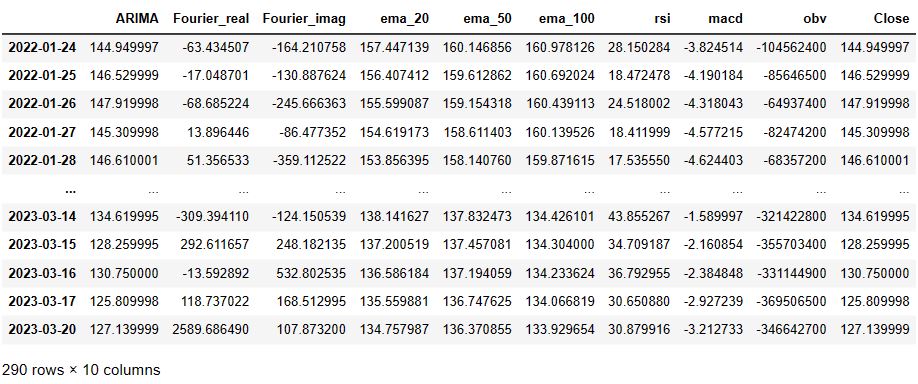
Let’s create the merged DF
merged_df = pd.concat([arima_df, fft_df_real, fft_df_imag, technical_indicators_df], axis=1)
merged_df = merged_df.dropna()
merged_df

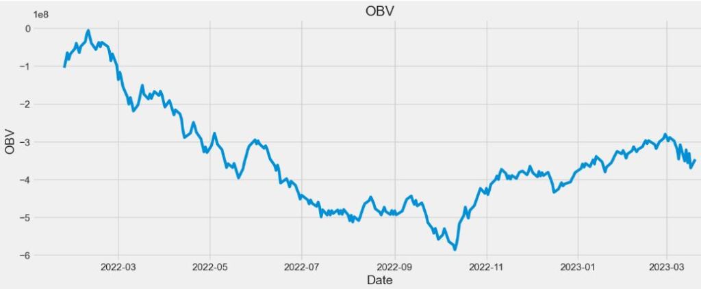
Let’s plot OBV

plt.figure(figsize=(16,6))
plt.title(‘OBV’)
plt.plot(merged_df[‘obv’])
plt.xlabel(‘Date’, fontsize=18)
plt.ylabel(‘OBV’, fontsize=18)

plt.show()

Let’s plot other TTIs against the stock price

import pandas as pd
import numpy as np

import matplotlib.pyplot as plt
import seaborn as sns
sns.set_style(‘whitegrid’)
plt.style.use(“fivethirtyeight”)
%matplotlib inline

from pandas_datareader.data import DataReader
import yfinance as yf
from pandas_datareader import data as pdr

yf.pdr_override()

from datetime import datetime

df = pdr.get_data_yahoo(‘JPM’, start=’2022-01-01′, end=datetime.now())

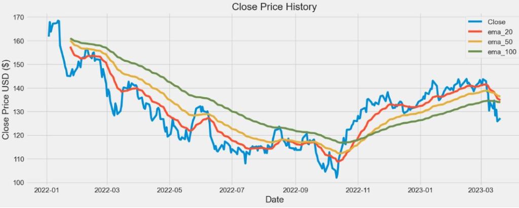
Let’s plot EMA TTI

plt.figure(figsize=(16,6))
plt.title(‘Close Price History’)
plt.plot(df[‘Close’])
plt.plot(merged_df[’ema_20′])
plt.plot(merged_df[’ema_50′])
plt.plot(merged_df[’ema_100′])
plt.legend([‘Close’, ’ema_20′,’ema_50′,’ema_100′], loc=’upper right’)
plt.xlabel(‘Date’, fontsize=18)
plt.ylabel(‘Close Price USD ($)’, fontsize=18)
plt.show()

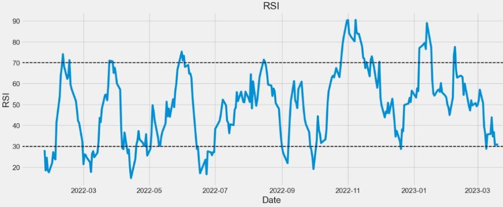
Let’s plot RSI TTI

plt.figure(figsize=(16,6))
plt.title(‘RSI’)
plt.plot(merged_df[‘rsi’])
plt.xlabel(‘Date’, fontsize=18)
plt.ylabel(‘RSI’, fontsize=18)
plt.axhline(30, linestyle = ‘–‘, linewidth = 1.5, color = ‘black’)
plt.axhline(70, linestyle = ‘–‘, linewidth = 1.5, color = ‘black’)
plt.show()

Let’s plot MACD TTI

def get_macd(price, slow, fast, smooth):
exp1 = price.ewm(span = fast, adjust = False).mean()
exp2 = price.ewm(span = slow, adjust = False).mean()
macd = pd.DataFrame(exp1 – exp2).rename(columns = {‘Close’:’macd’})
signal = pd.DataFrame(macd.ewm(span = smooth, adjust = False).mean()).rename(columns = {‘macd’:’signal’})
hist = pd.DataFrame(macd[‘macd’] – signal[‘signal’]).rename(columns = {0:’hist’})
frames = [macd, signal, hist]
df = pd.concat(frames, join = ‘inner’, axis = 1)
return df

googl_macd = get_macd(df[‘Close’], 26, 12, 9)
googl_macd.tail()

def plot_macd(prices, macd, signal, hist):
plt.figure(figsize=(16,6))

plt.plot(macd, color = 'black', linewidth = 1.5, label = 'MACD')
plt.plot(signal, color = 'blue', linewidth = 1.5, label = 'SIGNAL')

for i in range(len(prices)):
    if str(hist[i])[0] == '-':
        plt.bar(prices.index[i], hist[i], color = '#ef5350')
    else:
        plt.bar(prices.index[i], hist[i], color = '#26a69a')

plt.legend(loc = 'upper left')

plot_macd(df[‘Close’], googl_macd[‘macd’], googl_macd[‘signal’], googl_macd[‘hist’])

LSTM

Create a new dataframe with only the ‘Close column
data = df.filter([‘Close’])

dataset = data.values

training_data_len = int(np.ceil( len(dataset) * .95 ))

training_data_len

289

Let’s scale the data
from sklearn.preprocessing import MinMaxScaler

scaler = MinMaxScaler(feature_range=(0,1))
scaled_data = scaler.fit_transform(dataset)

Let’s create the scaled training data set

train_data = scaled_data[0:int(training_data_len), :]

x_train = []
y_train = []

for i in range(60, len(train_data)):
x_train.append(train_data[i-60:i, 0])
y_train.append(train_data[i, 0])
if i<= 61:
print(x_train)
print(y_train)
print()

x_train, y_train = np.array(x_train), np.array(y_train)

x_train = np.reshape(x_train, (x_train.shape[0], x_train.shape[1], 1))

Let’s build, compile and train the LSTM model

from keras.models import Sequential
from keras.layers import Dense, LSTM

model = Sequential()
model.add(LSTM(128, return_sequences=True, input_shape= (x_train.shape[1], 1)))
model.add(LSTM(64, return_sequences=False))
model.add(Dense(25))
model.add(Dense(1))

model.compile(optimizer=’adam’, loss=’mean_squared_error’)

history=model.fit(x_train, y_train, batch_size=1, epochs=32)

print(model.summary())

Model: "sequential_7"
_________________________________________________________________
 Layer (type)                Output Shape              Param #   
=================================================================
 lstm_6 (LSTM)               (None, 60, 128)           66560     
                                                                 
 lstm_7 (LSTM)               (None, 64)                49408     
                                                                 
 dense_18 (Dense)            (None, 25)                1625      
                                                                 
 dense_19 (Dense)            (None, 1)                 26        
                                                                 
=================================================================
Total params: 117,619
Trainable params: 117,619
Non-trainable params: 0
___________________________

Let’s create the testing data set

test_data = scaled_data[training_data_len – 60: , :]

x_test = []
y_test = dataset[training_data_len:, :]
for i in range(60, len(test_data)):
x_test.append(test_data[i-60:i, 0])

x_test = np.array(x_test)

x_test = np.reshape(x_test, (x_test.shape[0], x_test.shape[1], 1 ))

Let’s get the predicted price values

predictions = model.predict(x_test)
predictions = scaler.inverse_transform(predictions)

rmse = np.sqrt(np.mean(((predictions – y_test) ** 2)))
rmse

3.6409877950086997

Let’s calculate the test data metrics
y_pred=predictions
mse = mean_squared_error(y_test, y_pred)
rmse = np.sqrt(mse)
mae = mean_absolute_error(y_test, y_pred)

r2 = r2_score(y_test, y_pred)
evs = explained_variance_score(y_test, y_pred)

mape = np.mean(np.abs((y_test – y_pred) / y_test)) * 100
mpe = np.mean((y_test – y_pred) / y_test) * 100

print(f”Mean Squared Error (MSE): {mse}”)
print(f”Mean Absolute Error (MAE): {mae}”)
print(f”R2 Score: {r2}”)
print(f”Explained Variance Score: {evs}”)
print(f”Mean Absolute Percentage Error (MAPE): {mape}”)
print(f”Mean Percentage Error (MPE): {mpe}”)

Mean Squared Error (MSE): 13.256792123402313
Mean Absolute Error (MAE): 3.025512186686198
R2 Score: 0.64814314091558
Explained Variance Score: 0.6481807176153842
Mean Absolute Percentage Error (MAPE): 2.2817656702555715
Mean Percentage Error (MPE): -0.0674398726228619

Let’s visualize the data

train = data[:training_data_len]
valid = data[training_data_len:]
valid[‘Predictions’] = predictions

plt.figure(figsize=(16,6))
plt.title(‘Model’)
plt.xlabel(‘Date’, fontsize=18)
plt.ylabel(‘Close Price USD ($)’, fontsize=18)
plt.plot(train[‘Close’])
plt.plot(valid[[‘Close’, ‘Predictions’]])
plt.legend([‘Train’, ‘Val’, ‘Predictions’], loc=’lower right’)
plt.show()

Let’s plot the keys

print(history.history.keys())

dict_keys(['loss'])

plt.plot(history.history[‘loss’])
plt.ylabel(‘Loss’)
plt.xlabel(‘epoch’)

Finally, let’ print the validation and predicted prices
valid

Summary

We compared several techniques to predict the JPM stock price for 2022-2023.

1. The (Auto) ARIMA model was built using historical data to forecast future trends.
2. This best model ARIMA(0,1,0)(0,0,0)[0] was assessed using the SARIMAX comprehensive statistical output.
3. We invoked the FFT partial spectral decompositions of stock prices as model features.
4. We calculated s set of TTIs (EMA, RSI, MACD, and OBV) to validate the JPM trading breakouts.
5. The reliable LSTM model was built to predict stock prices with RMSE=3.6.
6. We assessed the LSTM performance using MSE, MAE, R2 score, explained variance score, MAPE, and MPE.

Continue Reading

Risk-Return Analysis and LSTM Price Predictions of 4 Major Tech Stocks in 2023

Revision 360 of Risk Aware Investing after SVB Collapse – 1. The Financial Sector

Portfolio max(Return/Risk) Stochastic Optimization of 20 Dividend Growth Stocks

SARIMAX X-Validation of EIA Crude Oil Prices Forecast in 2023 – 2. Brent

SARIMAX X-Validation of EIA Crude Oil Prices Forecast in 2023 – 1. WTI

SARIMAX-TSA Forecasting, QC and Visualization of E-Commerce Food Delivery Sales

Python Technical Analysis for BioTech – Get Buy Alerts on ABBV in 2023

Algo Trading Links

• The CodeX-Aroon Auto-Trading Approach – the AAPL Use Case

• DJI Market State Analysis using the Cruz Fitting Algorithm
• A TradeSanta’s Quick Guide to Best Swing Trading Indicators
• The Qullamaggie’s OXY Swing Breakouts
• The Qullamaggie’s TSLA Breakouts for Swing Traders
• Algorithmic Testing Stock Portfolios to Optimize the Risk/Reward Ratio
• Algorithmic Trading using Monte Carlo Predictions and 62 AI-Assisted Trading Technical Indicators (TTI)
• Basic Stock Price Analysis in Python
• S&P 500 Algorithmic Trading with FBProphet
• Predicting Trend Reversal in Algorithmic Trading using Stochastic Oscillator in Python
• Stock Forecasting with FBProphet
• Short-Term Stock Market Price Prediction using Deep Learning Models
• ML/AI Regression for Stock Prediction – AAPL Use Case
• Supervised ML/AI Stock Prediction using Keras LSTM Models

Stock Market Links

• A Comparative Analysis of The 3 Best U.S. Growth Stocks in Q1’23 – 1. WMT

• A Comparative Analysis of The 3 Best Global Growth Stocks in Q1’23 – 2. AZN
• Stocks to Watch in 2023: MarketBeat Ideas

• Zacks Investment Research Update Q4’22
• The Zacks Steady Investor – A Quick Look
• All Eyes on ETFs Sep ’22
• Zacks Insights into this High Inflation/Rising Rate Market
• SeekingAlpha Risk/Reward July Rundown
• Zacks Insights into the Commodity Bull Market
• Are Blue-Chips Perfect for This Bear Market?
• Bear Market Similarity Analysis using Nasdaq 100 Index Data
• AAPL Stock Technical Analysis 2 June 2022
• Inflation-Resistant Stocks to Buy
• A Weekday Market Research Update
• Stocks on Watch Tomorrow
• Stock Market ’22 Round Up & ’23 Outlook: Zacks Strategy vs Seeking Alpha Tactics

min(Risk/Reward Ratio) Links

• Towards min(Risk/Reward) – SeekingAlpha August Bear Market Update
• Upswing Resilient Investor Guide
• Investment Risk Management Study
• RISK AWARE INVESTMENT: GUIDE FOR EVERYONE 

Portfolio De-Risking Links

• Bear vs. Bull Portfolio Risk/Return Optimization QC Analysis
• Risk/Return POA – Dr. Dividend’s Positions
• Portfolio Optimization Risk/Return QC – Positions of Humble Div vs Dividend Glenn
• Risk/Return QC via Portfolio Optimization – Current Positions of The Dividend Breeder
• Stock Portfolio Risk/Return Optimization