Risk-Return Analysis and LSTM Price Predictions of 4 Major Tech Stocks in 2023

• Today we will walk through the Exploratory Data Analysis (EDA) and train the LSTM Sequential model by comparing Risk/Return of 4 major tech stocks in 2023: APPLE, GOOGLE, MICROSOFT, and AMAZON.

• Many of the most valuable companies in the world are technology companies. These 4 companies are some of the most dominant tech stocks that investors should consider.

• Recently, Amazon benefited from booming e-commerce sales as shoppers shied away from stores.
• Insatiable demand for PCs, smartphones, and other gadgets boosted sales for Microsoft and Apple.
• OpenAI’s ChatGPT took the world by storm in late 2022, and Microsoft is a major investor.
• Alphabet’s revenue growth slowed dramatically in 2022, with revenue up just 6% year over year in the third quarter. Alphabet’s Google Cloud business is growing rapidly, but its core advertising business is running up against a worsening economy.

The open-source Python workflow breaks down our investigation into the following 4 steps: (1) invoke yfinance to import real-time stock information into a Pandas dataframe; (2) visualize different dataframe columns with Seaborn and Matplotlib; (3) compare stock risk/return using historical data; (4) predict stock prices in 2023 with the trained LSTM model.

Input Data

Let’s set the working directory YOURPATH

import os
os.chdir(‘YOURPATH’)
os. getcwd()

and define the following tech stocks

tech_list = [‘AAPL’, ‘GOOG’, ‘MSFT’, ‘AMZN’]

Let’s read 1Y stock data

end = datetime.now()
start = datetime(end.year – 1, end.month, end.day)

for stock in tech_list:
globals()[stock] = yf.download(stock, start, end)

company_list = [AAPL, GOOG, MSFT, AMZN]
company_name = [“APPLE”, “GOOGLE”, “MICROSOFT”, “AMAZON”]

for company, com_name in zip(company_list, company_name):
company[“company_name”] = com_name

df = pd.concat(company_list, axis=0)
df.tail(10)

[*********************100%***********************]  1 of 1 completed
[*********************100%***********************]  1 of 1 completed
[*********************100%***********************]  1 of 1 completed
[*********************100%***********************]  1 of 1 completed

AAPL Summary Stats:
AAPL.describe()

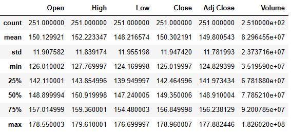
AAPL General info
AAPL.info()

<class 'pandas.core.frame.DataFrame'>
DatetimeIndex: 251 entries, 2022-03-11 to 2023-03-10
Data columns (total 7 columns):
 #   Column        Non-Null Count  Dtype  
---  ------        --------------  -----  
 0   Open          251 non-null    float64
 1   High          251 non-null    float64
 2   Low           251 non-null    float64
 3   Close         251 non-null    float64
 4   Adj Close     251 non-null    float64
 5   Volume        251 non-null    int64  
 6   company_name  251 non-null    object 
dtypes: float64(5), int64(1), object(1)
memory usage: 15.7+ KB

df.shape

(1004, 7)

Exploratory Data Analysis (EDA)

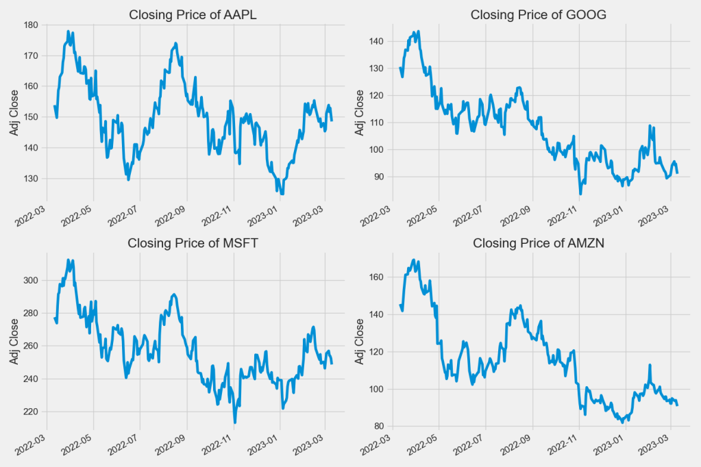
Let’s look at the closing price
plt.figure(figsize=(15, 10))
plt.subplots_adjust(top=1.25, bottom=1.2)

for i, company in enumerate(company_list, 1):
plt.subplot(2, 2, i)
company[‘Adj Close’].plot()
plt.ylabel(‘Adj Close’)
plt.xlabel(None)
plt.title(f”Closing Price of {tech_list[i – 1]}”)

plt.tight_layout()
plt.savefig(‘techclosingprice.png’)

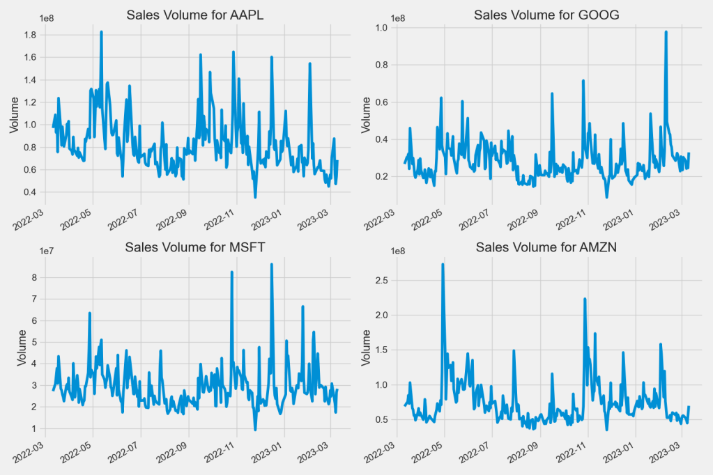
Now let’s plot the total volume of stock being traded each day
plt.figure(figsize=(15, 10))
plt.subplots_adjust(top=1.25, bottom=1.2)

for i, company in enumerate(company_list, 1):
plt.subplot(2, 2, i)
company[‘Volume’].plot()
plt.ylabel(‘Volume’)
plt.xlabel(None)
plt.title(f”Sales Volume for {tech_list[i – 1]}”)

plt.tight_layout()
plt.savefig(‘techvolume.png’)

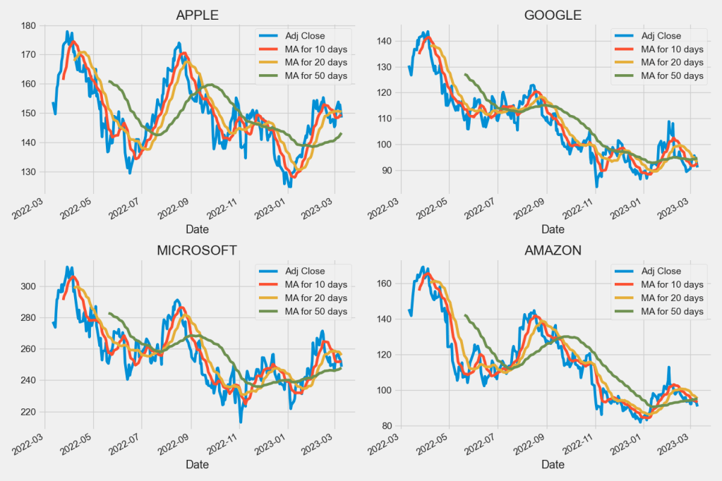
Moving Average (MA)

Let’s compute the Moving Average (MA) for 10, 20, and 50 days

ma_day = [10, 20, 50]

for ma in ma_day:
for company in company_list:
column_name = f”MA for {ma} days”
company[column_name] = company[‘Adj Close’].rolling(ma).mean()

fig, axes = plt.subplots(nrows=2, ncols=2)
fig.set_figheight(10)
fig.set_figwidth(15)

AAPL[[‘Adj Close’, ‘MA for 10 days’, ‘MA for 20 days’, ‘MA for 50 days’]].plot(ax=axes[0,0])
axes[0,0].set_title(‘APPLE’)

GOOG[[‘Adj Close’, ‘MA for 10 days’, ‘MA for 20 days’, ‘MA for 50 days’]].plot(ax=axes[0,1])
axes[0,1].set_title(‘GOOGLE’)

MSFT[[‘Adj Close’, ‘MA for 10 days’, ‘MA for 20 days’, ‘MA for 50 days’]].plot(ax=axes[1,0])
axes[1,0].set_title(‘MICROSOFT’)

AMZN[[‘Adj Close’, ‘MA for 10 days’, ‘MA for 20 days’, ‘MA for 50 days’]].plot(ax=axes[1,1])
axes[1,1].set_title(‘AMAZON’)

fig.tight_layout()
plt.savefig(‘techma102050.png’)

Daily Returns

We’ll use pct_change to find the percentage of Daily Return
for company in company_list:
company[‘Daily Return’] = company[‘Adj Close’].pct_change()

Then we’ll plot the the percentage of Daily Return
fig, axes = plt.subplots(nrows=2, ncols=2)
fig.set_figheight(10)
fig.set_figwidth(15)

AAPL[‘Daily Return’].plot(ax=axes[0,0], legend=True, linestyle=’–‘, marker=’o’)
axes[0,0].set_title(‘APPLE’)

GOOG[‘Daily Return’].plot(ax=axes[0,1], legend=True, linestyle=’–‘, marker=’o’)
axes[0,1].set_title(‘GOOGLE’)

MSFT[‘Daily Return’].plot(ax=axes[1,0], legend=True, linestyle=’–‘, marker=’o’)
axes[1,0].set_title(‘MICROSOFT’)

AMZN[‘Daily Return’].plot(ax=axes[1,1], legend=True, linestyle=’–‘, marker=’o’)
axes[1,1].set_title(‘AMAZON’)

fig.tight_layout()

plt.savefig(‘techdailyreturnpercentage.png’)

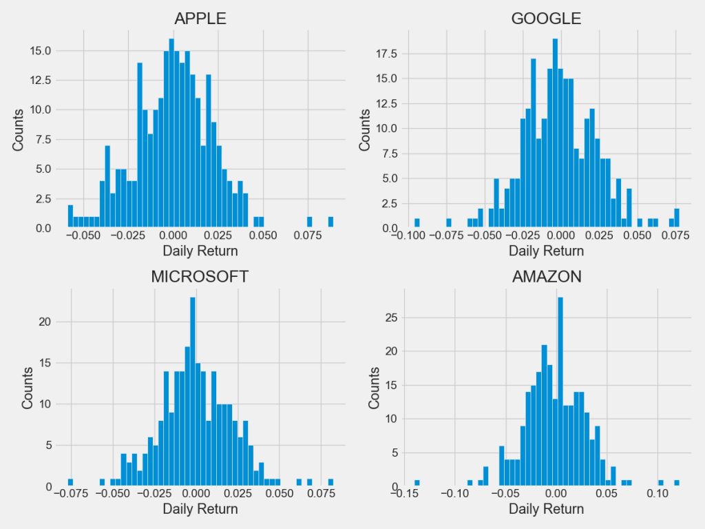
Let’s plot histograms of Daily Returns

plt.figure(figsize=(12, 9))

for i, company in enumerate(company_list, 1):
plt.subplot(2, 2, i)
company[‘Daily Return’].hist(bins=50)
plt.xlabel(‘Daily Return’)
plt.ylabel(‘Counts’)
plt.title(f'{company_name[i – 1]}’)

plt.tight_layout()
plt.savefig(‘techdailyreturnhistograms.png’)

Correlations

Let’ combine closing prices for 4 tech stocks into a single DataFrame

closing_df = pdr.get_data_yahoo(tech_list, start=start, end=end)[‘Adj Close’]

and compute their daily returns
tech_rets = closing_df.pct_change()
tech_rets.head()

[*********************100%***********************]  4 of 4 completed

We’ll use joinplot to compare the daily returns of Google and Microsoft
sns.jointplot(x=’GOOG’, y=’MSFT’, data=tech_rets, kind=’scatter’)
plt.savefig(‘techdailyreturngoogmsft.png’)

Similarly, we can compare the daily returns of AMZN and Microsoft
sns.jointplot(x=’AMZN’, y=’MSFT’, data=tech_rets, kind=’scatter’)
plt.savefig(‘techdailyreturnamznmsft.png’)

Similarly, we can compare the daily returns of AMZN and AAPL

sns.jointplot(x=’AMZN’, y=’AAPL’, data=tech_rets, kind=’scatter’)
plt.savefig(‘techdailyreturnamznappl.png’)

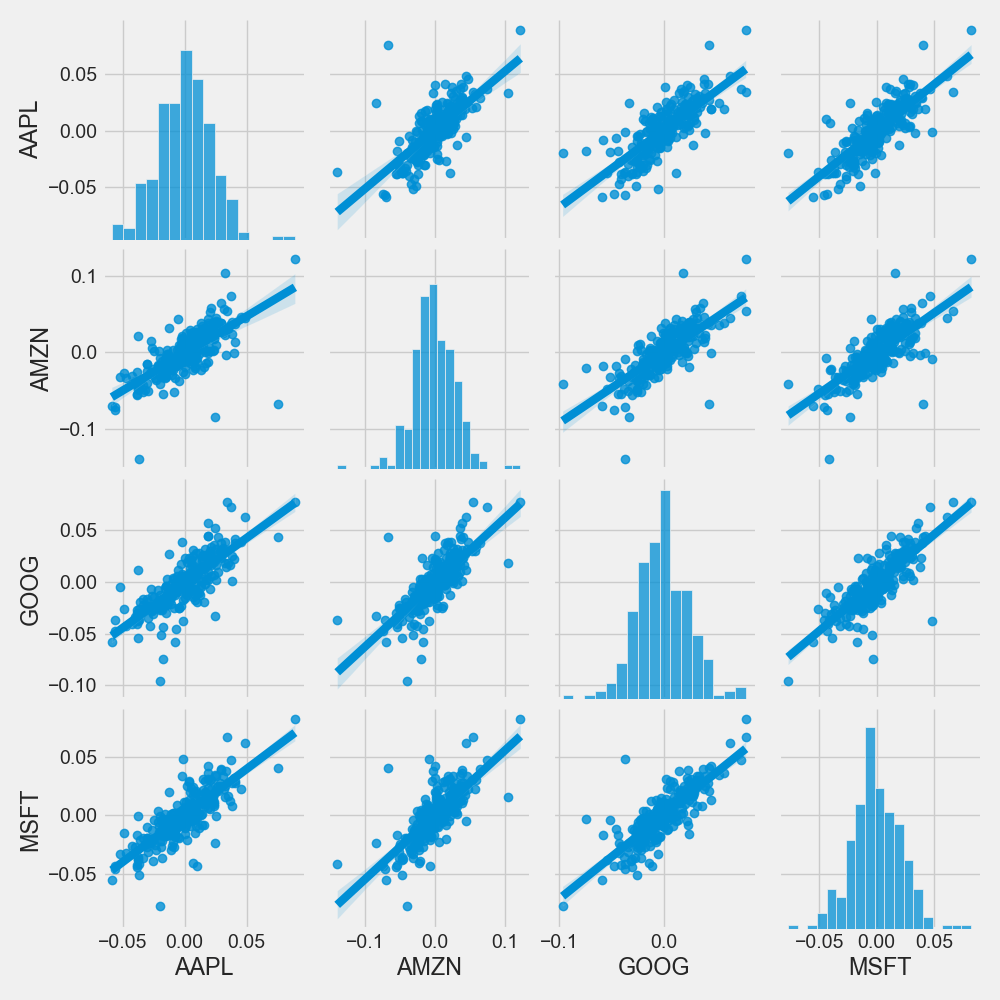
Let’s use pairplot as follows

sns.pairplot(tech_rets, kind=’reg’)
plt.savefig(‘techdailyreturnpairplot.png’)

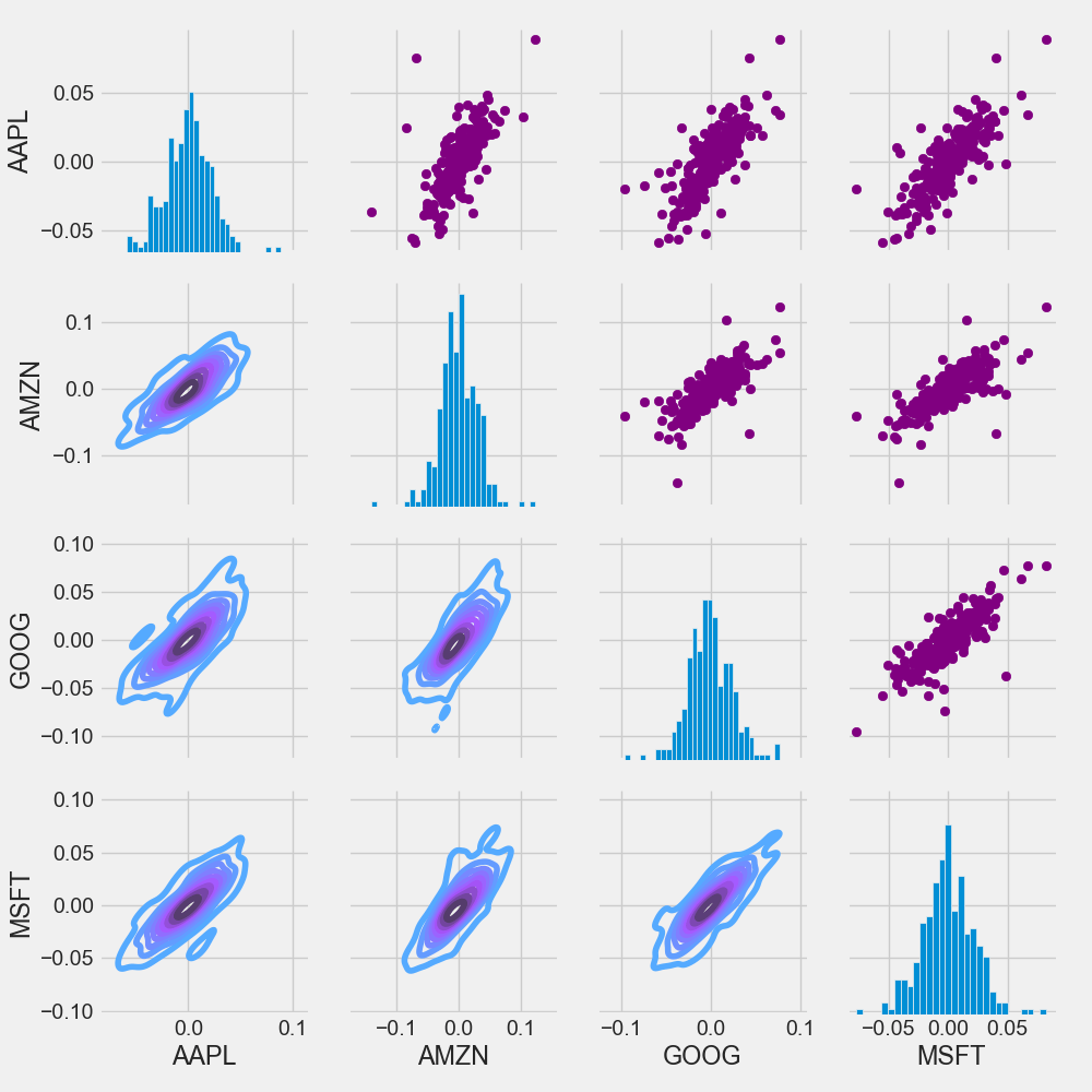
Let’s combine PairGrid, map_upper, map_lower, and map_diag into a single plot

return_fig = sns.PairGrid(tech_rets.dropna())

return_fig.map_upper(plt.scatter, color=’purple’)

return_fig.map_lower(sns.kdeplot, cmap=’cool_d’)

return_fig.map_diag(plt.hist, bins=30)
plt.savefig(‘techmappairgrid.png’)

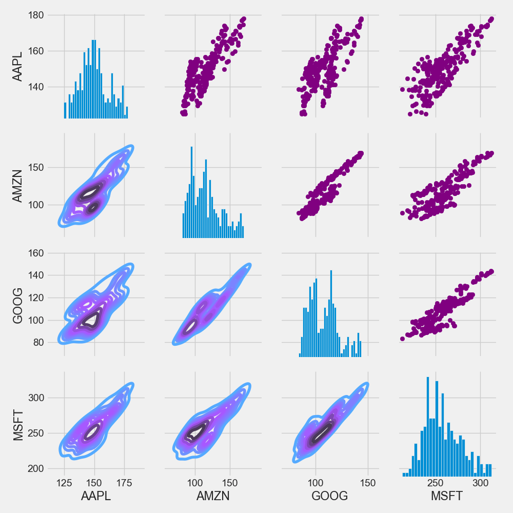
Similarly, we can plot the closing price instead of daily returns

returns_fig = sns.PairGrid(closing_df)

returns_fig.map_upper(plt.scatter,color=’purple’)

returns_fig.map_lower(sns.kdeplot,cmap=’cool_d’)

returns_fig.map_diag(plt.hist,bins=30)
plt.savefig(‘techmappairgridclosingprice.png’)

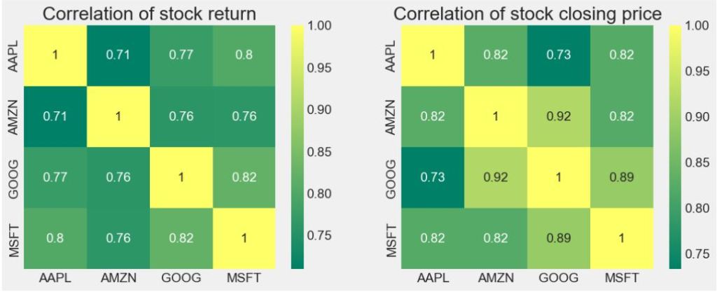
Let’s plot the correlation matrix of stock returns vs closing price

plt.figure(figsize=(12, 10))

plt.subplot(2, 2, 1)
sns.heatmap(tech_rets.corr(), annot=True, cmap=’summer’)
plt.title(‘Correlation of stock return’)

plt.subplot(2, 2, 2)
sns.heatmap(closing_df.corr(), annot=True, cmap=’summer’)
plt.title(‘Correlation of stock closing price’)
plt.savefig(‘techcorrmatrixreturnclosingprice.png’)

Risk-Return Analysis

How much value do we put at risk by investing in a particular stock? Let’s look at the Risk-Return map
rets = tech_rets.dropna()

area = np.pi * 20

plt.figure(figsize=(10, 8))
plt.scatter(rets.mean(), rets.std(), s=area)
plt.xlabel(‘Expected return’)
plt.ylabel(‘Risk’)

for label, x, y in zip(rets.columns, rets.mean(), rets.std()):
plt.annotate(label, xy=(x, y), xytext=(50, 50), textcoords=’offset points’, ha=’right’, va=’bottom’,
arrowprops=dict(arrowstyle=’-‘, color=’blue’, connectionstyle=’arc3,rad=-0.3′))
plt.savefig(‘techstockriskreturnmap.png’)

AAPL Price LSTM Model

Predicting the closing price stock price of APPLE inc.

Let’s get the stock quote
df = pdr.get_data_yahoo(‘AAPL’, start=’2022-01-03′, end=datetime.now())

[*********************100%***********************]  1 of 1 completed

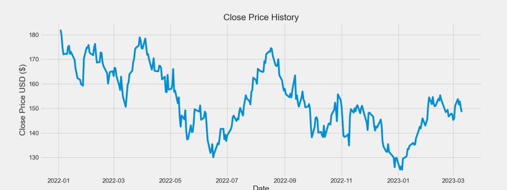
Let’s plot the AAPL close price USD 1Y history

plt.figure(figsize=(16,6))
plt.title(‘Close Price History’)
plt.plot(df[‘Close’])
plt.xlabel(‘Date’, fontsize=18)
plt.ylabel(‘Close Price USD ($)’, fontsize=18)
plt.savefig(‘aaplclosignprice.png’)

Creating a new dataframe with only the ‘Close’ column
data = df.filter([‘Close’])

Convert the dataframe to a numpy array
dataset = data.values

Get the number of rows to train the model on
training_data_len = int(np.ceil( len(dataset) * .95 ))

training_data_len

284

Let’s scale the data
from sklearn.preprocessing import MinMaxScaler

scaler = MinMaxScaler(feature_range=(0,1))
scaled_data = scaler.fit_transform(dataset)

Create the scaled training data set
train_data = scaled_data[0:int(training_data_len), :]

Split the data into x_train and y_train data sets
x_train = []
y_train = []

for i in range(60, len(train_data)):
x_train.append(train_data[i-60:i, 0])
y_train.append(train_data[i, 0])
if i<= 61:
print(x_train)
print(y_train)
print()

Convert the x_train and y_train to numpy arrays
x_train, y_train = np.array(x_train), np.array(y_train)

Reshape the data
x_train = np.reshape(x_train, (x_train.shape[0], x_train.shape[1], 1))

Let’s build, compile and train the LSTM model

from keras.models import Sequential
from keras.layers import Dense, LSTM

model = Sequential()
model.add(LSTM(128, return_sequences=True, input_shape= (x_train.shape[1], 1)))
model.add(LSTM(64, return_sequences=False))
model.add(Dense(25))
model.add(Dense(1))

model.compile(optimizer=’adam’, loss=’mean_squared_error’)

model.fit(x_train, y_train, batch_size=1, epochs=20)

Epoch 1/20
224/224 [==============================] - 5s 13ms/step - loss: 0.0174
Epoch 2/20
224/224 [==============================] - 3s 13ms/step - loss: 0.0078
Epoch 3/20
224/224 [==============================] - 3s 13ms/step - loss: 0.0067
Epoch 4/20
224/224 [==============================] - 3s 13ms/step - loss: 0.0055
Epoch 5/20
224/224 [==============================] - 3s 12ms/step - loss: 0.0063
Epoch 6/20
224/224 [==============================] - 3s 13ms/step - loss: 0.0049
Epoch 7/20
224/224 [==============================] - 3s 13ms/step - loss: 0.0048
Epoch 8/20
224/224 [==============================] - 3s 13ms/step - loss: 0.0045
Epoch 9/20
224/224 [==============================] - 3s 13ms/step - loss: 0.0043
Epoch 10/20
224/224 [==============================] - 3s 13ms/step - loss: 0.0044
Epoch 11/20
224/224 [==============================] - 3s 13ms/step - loss: 0.0043
Epoch 12/20
224/224 [==============================] - 3s 13ms/step - loss: 0.0050
Epoch 13/20
224/224 [==============================] - 3s 13ms/step - loss: 0.0045
Epoch 14/20
224/224 [==============================] - 4s 17ms/step - loss: 0.0051
Epoch 15/20
224/224 [==============================] - 3s 15ms/step - loss: 0.0047
Epoch 16/20
224/224 [==============================] - 3s 14ms/step - loss: 0.0043
Epoch 17/20
224/224 [==============================] - 3s 14ms/step - loss: 0.0040
Epoch 18/20
224/224 [==============================] - 3s 14ms/step - loss: 0.0040
Epoch 19/20
224/224 [==============================] - 3s 15ms/step - loss: 0.0048
Epoch 20/20
224/224 [==============================] - 4s 16ms/step - loss: 0.0043

Out[84]:

<keras.callbacks.History at 0x1d91f3eadc0>

history = model.history.history
print(history)

{'loss': [0.017397716641426086, 0.007797327823936939, 0.0067240772768855095, 0.005469697993248701, 0.0062720817513763905, 0.004899029619991779, 0.0048156785778701305, 0.004509173333644867, 0.00425869133323431, 0.004385276231914759, 0.004279236309230328, 0.004953560419380665, 0.004468429367989302, 0.00513608381152153, 0.004718478303402662, 0.004269555676728487, 0.00395335303619504, 0.004049328621476889, 0.004776121117174625, 0.004271872341632843]}

Let’s plot the LSTM loss vs epoch<20

import math
from matplotlib import pyplot as plt
epoch = np.arange(len(history[‘loss’])) + 1
new_list = range(math.floor(min(epoch)), math.ceil(max(epoch))+1)
plt.xticks(new_list)
histloss=history[‘loss’]
plt.plot(epoch,histloss)
plt.xlabel(“Epoch”)
plt.ylabel(“Loss”)

plt.title(“LSTM History Loss”)
plt.savefig(‘lstmhistoryloss.png’)

Let’s create the testing data set

test_data = scaled_data[training_data_len – 60: , :]

x_test = []
y_test = dataset[training_data_len:, :]
for i in range(60, len(test_data)):
x_test.append(test_data[i-60:i, 0])

Convert the data to a numpy array
x_test = np.array(x_test)

Reshape the data
x_test = np.reshape(x_test, (x_test.shape[0], x_test.shape[1], 1 ))

Get the predicted price values
predictions = model.predict(x_test)
predictions = scaler.inverse_transform(predictions)

Get the root mean squared error (RMSE)
rmse = np.sqrt(np.mean(((predictions – y_test) ** 2)))
rmse

1/1 [==============================] - 0s 427ms/step

Out[92]:

2.7391927142048043

Plot the data:
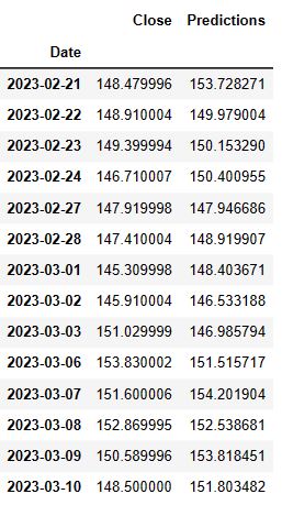
train = data[:training_data_len]
valid = data[training_data_len:]
valid[‘Predictions’] = predictions

plt.figure(figsize=(16,6))
plt.title(‘Model’)
plt.xlabel(‘Date’, fontsize=18)
plt.ylabel(‘Close Price USD ($)’, fontsize=18)
plt.plot(train[‘Close’])
plt.plot(valid[[‘Close’, ‘Predictions’]])
plt.legend([‘Train’, ‘Val’, ‘Predictions’], loc=’lower right’)
plt.savefig(‘aapllstmprediction.png’)

Show the valid and predicted prices
valid

Summary

• In this study, we performed EDA, correlations between different stocks, risk-return value assessment and LSTM model predictions of tech stock prices and their daily returns.

• We believe that this research helps in understanding the underlying patterns and relationships in the stock data. Here we examined the patterns in the stock price of AAPL, AMZN, MSFT, and GOOG.
• We have shown that major tech stocks are positively correlated in that they move up or down in tandem. Stock correlation is important because it can help show an investor that they may not be as diversified as they think.
• We have focused on making short-term predictions to get a probabilistic estimate of what the tech stock “could” look like soon. With enough historical data and useful features, LSTM models might predict short-term fluctuations in the market for an average, uneventful market day.

Explore More

• Portfolio max(Return/Risk) Stochastic Optimization of 20 Dividend Growth Stocks
• The Donchian Channel vs Buy-and-Hold Breakout Trading Systems – $MO Use-Case
• Towards Max(ROI/Risk) Trading in Q1 2023
• A Comparative Analysis of The 3 Best U.S. Growth Stocks in Q1’23 – 1. WMT
• A Comparative Analysis of The 3 Best Global Growth Stocks in Q1’23 – 2. AZN
• A Comparative Analysis of The 3 Best U.S. Growth Stocks in Q1’23 – 3. LYTS
• SARIMAX X-Validation of EIA Crude Oil Prices Forecast in 2023 – 2. Brent
• SARIMAX X-Validation of EIA Crude Oil Prices Forecast in 2023 – 1. WTI
• Stocks to Watch in 2023: MarketBeat Ideas
• SARIMAX-TSA Forecasting, QC and Visualization of E-Commerce Food Delivery Sales
• Python Technical Analysis for BioTech – Get Buy Alerts on ABBV in 2023
• Biotech Genmab Hold Alert via Fibonacci Retracement Trading Simulations
• Stock Market ’22 Round Up & ’23 Outlook: Zacks Strategy vs Seeking Alpha Tactics
• The CodeX-Aroon Auto-Trading Approach – the AAPL Use Case
• DJI Market State Analysis using the Cruz Fitting Algorithm
• Cloud-Native Tech Autumn 2022 Fair
• Bear vs. Bull Portfolio Risk/Return Optimization QC Analysis
• Technology Focus Weekly Update 16 Oct ’22
• A TradeSanta’s Quick Guide to Best Swing Trading Indicators
• Risk/Return POA – Dr. Dividend’s Positions
• Portfolio Optimization Risk/Return QC – Positions of Humble Div vs Dividend Glenn
• Risk/Return QC via Portfolio Optimization – Current Positions of The Dividend Breeder
• Stock Portfolio Risk/Return Optimization
• The Qullamaggie’s OXY Swing Breakouts
• Towards min(Risk/Reward) – SeekingAlpha August Bear Market Update
• Algorithmic Testing Stock Portfolios to Optimize the Risk/Reward Ratio
• Are Blue-Chips Perfect for This Bear Market?
• Bear Market Similarity Analysis using Nasdaq 100 Index Data
• Predicting Trend Reversal in Algorithmic Trading using Stochastic Oscillator in Python
• Inflation-Resistant Stocks to Buy
• ML/AI Regression for Stock Prediction – AAPL Use Case
• Supervised ML/AI Stock Prediction using Keras LSTM Models
• Upswing Resilient Investor Guide
• Macroaxis Wealth Optimization
• AI-Driven Stock Prediction using Keras LSTM Models
• Investment Risk Management Study
• Stocks on Watch Tomorrow
• Short-Term Stock Market Price Prediction using Deep Learning Models
• A Weekday Market Research Update

---