
- Cancer is the common problem for all people in the world with all types. Particularly, Breast Cancer (BC) is the most frequent disease as a cancer type for women.
- Therefore, any development for diagnosis and prediction of BC disease is capital important for public health.
- AI Health uses the power of Machine Learning (ML) and Artificial Intelligence (AI) to accelerate the process of early diagnosis and prediction of BC.
- In this post, 12 of the most popular ML techniques have been used for BC binary classification. The performance of these techniques have been conducted using available QC/QA and cross-validation metrics.
- Our current aim is to assess pros and cons of different ML models in BC prediction.
- The overall objective is to promote the integration of ML and public health to improve BC clinical diagnostic accuracy.
Contents:
- BC Dataset
- Cross-Validation Score
- Classification Report
- Learning Curves
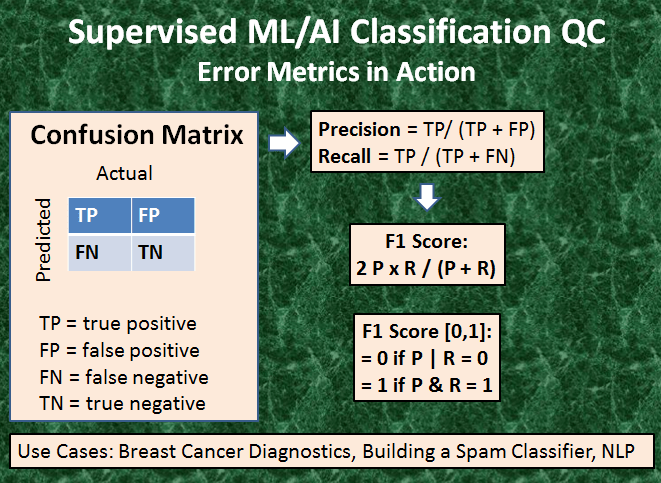
- Confusion Matrix
- from confusion matrix calculate accuracy
- from confusion matrix calculate accuracy
- * The specificity of a test is its ability to designate an individual who does not have a disease as negative.
- * A highly specific test means that there are few false positive results.
- * Sensitivity is the indicator on the ability of screening to find cancer in the detectable preclinical phase (DPCP).
- * The ability is usually specified as to the screening test.
- Accuracy-Precision-Recall-Cohen-F1 KPIs
- Other Performance Matrics
- Conclusions
- Explore More
- Embed Socials
- Infographic
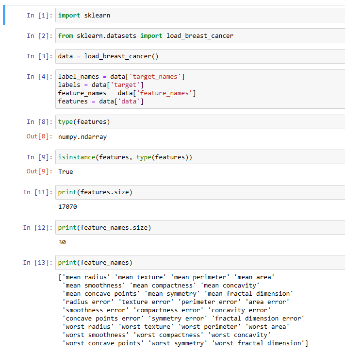
BC Dataset
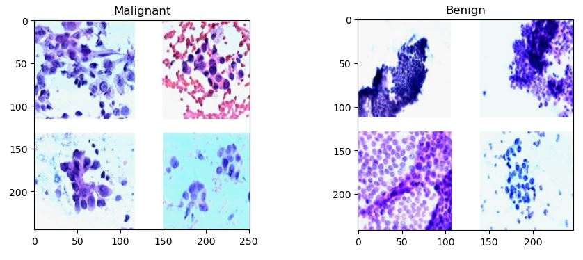
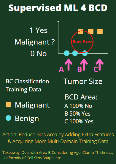
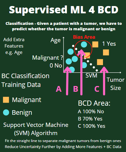
Conventionally, the Breast Cancer Wisconsin (Diagnostic) Data Set has been used to predict whether the breast cancer is benign or malignant. Features were computed from a digitized image of a fine needle aspirate (FNA) of a breast mass. They describe characteristics of the cell nuclei present in the image.
The dataset can be found on UCI ML Repository.
Attribute Information:
1) ID number
2) Diagnosis (M = malignant, B = benign)
3-32)
Ten real-valued features are computed for each cell nucleus:
a) radius (mean of distances from center to points on the perimeter)
b) texture (standard deviation of gray-scale values)
c) perimeter
d) area
e) smoothness (local variation in radius lengths)
f) compactness (perimeter^2 / area – 1.0)
g) concavity (severity of concave portions of the contour)
h) concave points (number of concave portions of the contour)
i) symmetry
j) fractal dimension (“coastline approximation” – 1)
The mean, standard error and “worst” or largest (mean of the three
largest values) of these features were computed for each image,
resulting in 30 features. For instance, field 3 is Mean Radius, field
13 is Radius SE, field 23 is Worst Radius.
All feature values are recoded with four significant digits.
Missing attribute values: none
Class distribution: 357 benign (B), 212 malignant (M).

Cross-Validation Score
The K-fold cross-validation (CV) workflow consists of the following steps:
import libraries, get BC data, normalize the data, apply BC classifiers, and get CV scores.
Let’s set the working directory YOURPATH
import os
os.chdir(‘YOURPATH’) # Set working directory
os. getcwd()
Let’s import the key libraries
import numpy as np
from sklearn.datasets import load_breast_cancer
from sklearn.preprocessing import MinMaxScaler
from sklearn.linear_model import LogisticRegression
from sklearn.model_selection import cross_val_score
load the BC data
cancer = load_breast_cancer()
X_cancer = cancer['data']
y_cancer = cancer['target']
normalized the data
scaler = MinMaxScaler()
X_cancer_scaled = scaler.fit_transform(X_cancer)
apply the LR classifier
clf = LogisticRegression()
and get the CV scores
cv_scores = cross_val_score(clf, X_cancer_scaled, y_cancer, cv = 5)

print('Cross validation scores (5 folds): {}'.format(cv_scores))
print('The average cross validation score (5 folds): {}'.format(np.mean(cv_scores)))
Cross validation scores (5 folds): [0.95614035 0.96491228 0.97368421 0.95614035 0.96460177]
The average cross validation score (5 folds): 0.9630957925787922
Let’s look at the GaussianNB classifier
from sklearn.naive_bayes import GaussianNB
estimator = GaussianNB()
cv_scores = cross_val_score(estimator, X_cancer_scaled, y_cancer, cv = 5)
print(‘Cross validation scores (5 folds): {}’.format(cv_scores))
print(‘The average cross validation score (5 folds): {}’.format(np.mean(cv_scores)))
Cross validation scores (5 folds): [0.90350877 0.9122807  0.95614035 0.94736842 0.92035398]
The average cross validation score (5 folds): 0.927930445582984
Let’s look at the SVC classifier
from sklearn.svm import SVC
estimator = SVC()
cv_scores = cross_val_score(estimator, X_cancer_scaled, y_cancer, cv = 5)
print(‘Cross validation scores (5 folds): {}’.format(cv_scores))
print(‘The average cross validation score (5 folds): {}’.format(np.mean(cv_scores)))
Cross validation scores (5 folds): [0.96491228 0.96491228 0.99122807 0.96491228 0.98230088]
The average cross validation score (5 folds): 0.9736531594472908
Let’s look at the KNeighborsClassifier
from sklearn.neighbors import KNeighborsClassifier
logreg = KNeighborsClassifier(n_neighbors=6)
cv_scores = cross_val_score(logreg, X_cancer_scaled, y_cancer, cv = 5)
print(‘Cross validation scores (5 folds): {}’.format(cv_scores))
print(‘The average cross validation score (5 folds): {}’.format(np.mean(cv_scores)))
Cross validation scores (5 folds): [0.95614035 0.94736842 0.99122807 0.96491228 0.96460177]
The average cross validation score (5 folds): 0.9648501785437043
Let’s invoke more sklearn classifiers
from sklearn.ensemble import RandomForestClassifier, GradientBoostingClassifier, ExtraTreesClassifier
estimator = RandomForestClassifier()
cv_scores = cross_val_score(estimator, X_cancer_scaled, y_cancer, cv = 5)
print(‘Cross validation scores (5 folds): {}’.format(cv_scores))
print(‘The average cross validation score (5 folds): {}’.format(np.mean(cv_scores)))
Cross validation scores (5 folds): [0.92982456 0.94736842 0.99122807 0.97368421 0.97345133]
The average cross validation score (5 folds): 0.9631113181183046
estimator = GradientBoostingClassifier()
cv_scores = cross_val_score(estimator, X_cancer_scaled, y_cancer, cv = 5)
print(‘Cross validation scores (5 folds): {}’.format(cv_scores))
print(‘The average cross validation score (5 folds): {}’.format(np.mean(cv_scores)))
Cross validation scores (5 folds): [0.92982456 0.93859649 0.97368421 0.98245614 0.98230088]
The average cross validation score (5 folds): 0.9613724576929048
Cross validation scores (5 folds): [0.92982456 0.93859649 0.97368421 0.98245614 0.98230088]
The average cross validation score (5 folds): 0.9613724576929048
estimator = ExtraTreesClassifier()
cv_scores = cross_val_score(estimator, X_cancer_scaled, y_cancer, cv = 5)
print(‘Cross validation scores (5 folds): {}’.format(cv_scores))
print(‘The average cross validation score (5 folds): {}’.format(np.mean(cv_scores)))
Cross validation scores (5 folds): [0.94736842 0.96491228 0.98245614 0.97368421 0.96460177]
The average cross validation score (5 folds): 0.9666045645086166
Here is the summary table based on the average CV score
| Nr | Method | mean CV score | CV Rank |
| 1 | LR | 0.963 | 3 |
| 2 | GNB | 0.928 | 5 |
| 3 | SVC | 0.973 | 1 |
| 4 | KNN | 0.965 | 2 |
| 5 | RF | 0.963 | 3 |
| 6 | GB | 0.961 | 4 |
| 7 | ET | 0.966 | 2 |
Classification Report
Let’s import the key libraries and prepare the input BC data
import matplotlib.pyplot as plt
from sklearn.datasets import load_breast_cancer
dataset = load_breast_cancer(as_frame=True)
X = dataset[‘data’]
y = dataset[‘target’]
dataset[‘data’].head()

Let’s check the target variable
dataset[‘target’].value_counts()
1    357
0    212
Name: target, dtype: int64
Let’s perform train/test data split with test_size=0.25
from sklearn.model_selection import train_test_split
X_train, X_test, y_train, y_test = train_test_split(X, y , test_size=0.25, random_state=0)
Let’s apply RobustScaler to our data
from sklearn.preprocessing import RobustScaler
ss_train = RobustScaler()
X_train = ss_train.fit_transform(X_train)
ss_test = RobustScaler()
X_test = ss_test.fit_transform(X_test)
Let’s compare several classifiers in terms of the accuracy score
from sklearn.neighbors import KNeighborsClassifier
modelknn = KNeighborsClassifier(n_neighbors=6)
modelknn.fit(X_train, y_train)
modelknn.score(X_test, y_test)
KNN accuracy score:
0.9440559440559441
Let’s make KNN predictions
predictions = modelknn.predict(X_test)
and calculate the confusion matrix
from sklearn.metrics import confusion_matrix
cm = confusion_matrix(y_test, predictions)
TN, FP, FN, TP = confusion_matrix(y_test, predictions).ravel()
print(‘True Positive(TP) = ‘, TP)
print(‘False Positive(FP) = ‘, FP)
print(‘True Negative(TN) = ‘, TN)
print(‘False Negative(FN) = ‘, FN)
True Positive(TP)  =  88
False Positive(FP) =  6
True Negative(TN)  =  47
False Negative(FN) =  2
The accuracy score is given by
accuracy = (TP + TN) / (TP + FP + TN + FN)
print(‘Accuracy of the binary classifier = {:0.3f}’.format(accuracy))
Accuracy of the binary classifier = 0.944
Let’s look at several ML models
models = {}
Logistic Regression
from sklearn.linear_model import LogisticRegression
models[‘Logistic Regression’] = LogisticRegression()
Support Vector Machines
from sklearn.svm import LinearSVC
models[‘Support Vector Machines’] = LinearSVC()
Decision Trees
from sklearn.tree import DecisionTreeClassifier
models[‘Decision Trees’] = DecisionTreeClassifier()
Random Forest
from sklearn.ensemble import RandomForestClassifier
models[‘Random Forest’] = RandomForestClassifier()
Naive Bayes
from sklearn.naive_bayes import GaussianNB
models[‘Naive Bayes’] = GaussianNB()
K-Nearest Neighbors
from sklearn.neighbors import KNeighborsClassifier
models[‘K-Nearest Neighbor’] = KNeighborsClassifier()
Let’s calculate the accuracy, precision and recall scores for these classifiers
from sklearn.metrics import accuracy_score, precision_score, recall_score
accuracy, precision, recall = {}, {}, {}
for key in models.keys():
# Fit the classifier
models[key].fit(X_train, y_train)

# Make predictions
predictions = models[key].predict(X_test)

# Calculate metrics
accuracy[key] = accuracy_score(predictions, y_test)
precision[key] = precision_score(predictions, y_test)
recall[key] = recall_score(predictions, y_test)
import pandas as pd
df_model = pd.DataFrame(index=models.keys(), columns=[‘Accuracy’, ‘Precision’, ‘Recall’])
df_model[‘Accuracy’] = accuracy.values()
df_model[‘Precision’] = precision.values()
df_model[‘Recall’] = recall.values()
df_model

Let’s create the corresponding bar chart

From this comparison it follows that KNN returns the best precision score of 98.8%, whereas Logistic Regression performs the best in terms of the accuracy and recall scores of 97.2% and 97.7%, respectively.
Let’s further expand the list of classifiers
modelss = {}
Logistic Regression
from sklearn.linear_model import LogisticRegression
modelss[‘Logistic Regression’] = LogisticRegression()
Support Vector Machines
from sklearn.svm import LinearSVC
modelss[‘Support Vector Machines’] = LinearSVC()
Decision Trees
from sklearn.tree import DecisionTreeClassifier
modelss[‘Decision Trees’] = DecisionTreeClassifier()
Random Forest
from sklearn.ensemble import RandomForestClassifier
modelss[‘Random Forest’] = RandomForestClassifier()
Naive Bayes
from sklearn.naive_bayes import GaussianNB
modelss[‘Naive Bayes’] = GaussianNB()
K-Nearest Neighbors
from sklearn.neighbors import KNeighborsClassifier
modelss[‘K-Nearest Neighbor’] = KNeighborsClassifier()
MLP
modelss[‘MLP’] = MLPClassifier(alpha=1, max_iter=1000)
modelss[‘GP’] = GaussianProcessClassifier(1.0 * RBF(1.0))
modelss[‘Ada’] = AdaBoostClassifier()
modelss[‘GNB’] = GaussianNB()
modelss[‘QDA’] = QuadraticDiscriminantAnalysis()
Let’s fit/train the classifier, make test predictions, and compute key metrics
from sklearn.metrics import accuracy_score, precision_score, recall_score
accuracy, precision, recall = {}, {}, {}
for key in modelss.keys():
# Fit the classifier
modelss[key].fit(X_train, y_train)

# Make predictions
predictions = modelss[key].predict(X_test)

# Calculate metrics
accuracy[key] = accuracy_score(predictions, y_test)
precision[key] = precision_score(predictions, y_test)
recall[key] = recall_score(predictions, y_test)
import pandas as pd
df_model = pd.DataFrame(index=modelss.keys(), columns=[‘Accuracy’, ‘Precision’, ‘Recall’])
df_model[‘Accuracy’] = accuracy.values()
df_model[‘Precision’] = precision.values()
df_model[‘Recall’] = recall.values()
df_model
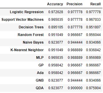
Let’s create the corresponding bar chart

From this comparison it follows that KNN and MLP return the best precision score of 98.8%, whereas Logistic Regression still performs the best in terms of the accuracy and recall scores.
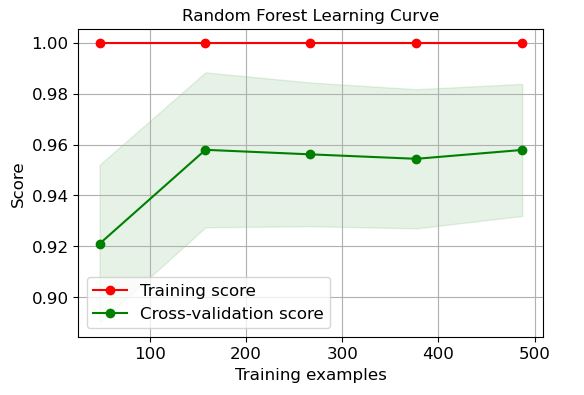
Learning Curves
Let’s look at the scikitplot learning curves
import scikitplot as skplt
import sklearn
from sklearn.datasets import load_digits, load_boston, load_breast_cancer
from sklearn.model_selection import train_test_split
from sklearn.ensemble import RandomForestClassifier, RandomForestRegressor, GradientBoostingClassifier, ExtraTreesClassifier
from sklearn.linear_model import LinearRegression, LogisticRegression
from sklearn.cluster import KMeans
from sklearn.decomposition import PCA
import matplotlib.pyplot as plt
import sys
import warnings
warnings.filterwarnings(“ignore”)
print(“Scikit Plot Version : “, skplt.version)
print(“Scikit Learn Version : “, sklearn.version)
print(“Python Version : “, sys.version)
%matplotlib inline
Scikit Plot Version :  0.3.7
Scikit Learn Version :  1.1.3
Python Version :  3.9.13 (main, Aug 25 2022, 23:51:50) [MSC v.1916 64 bit (AMD64)]
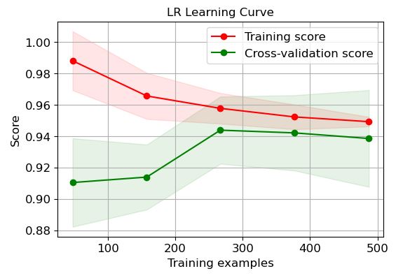
LR:
logreg=modelss[‘Logistic Regression’]
skplt.estimators.plot_learning_curve(logreg, X, y,
cv=7, shuffle=True, scoring=”accuracy”,
n_jobs=-1, figsize=(6,4), title_fontsize=”large”, text_fontsize=”large”,
title=”LR Learning Curve”);
plt.savefig(‘learningcurvelr.png’, dpi=300, bbox_inches=’tight’)
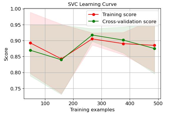
SVC:
logreg=modelss[‘Support Vector Machines’]
skplt.estimators.plot_learning_curve(logreg, X, y,
cv=7, shuffle=True, scoring=”accuracy”,
n_jobs=-1, figsize=(6,4), title_fontsize=”large”, text_fontsize=”large”,
title=”SVC Learning Curve”);
plt.savefig(‘learningcurvesvc.png’, dpi=300, bbox_inches=’tight’)
DT:
logreg=modelss[‘Decision Trees’]
skplt.estimators.plot_learning_curve(logreg, X, y,
cv=7, shuffle=True, scoring=”accuracy”,
n_jobs=-1, figsize=(6,4), title_fontsize=”large”, text_fontsize=”large”,
title=”DT Learning Curve”);
plt.savefig(‘learningcurvedt.png’, dpi=300, bbox_inches=’tight’)

RF:
logreg=modelss[‘Random Forest’]
skplt.estimators.plot_learning_curve(logreg, X, y,
cv=7, shuffle=True, scoring=”accuracy”,
n_jobs=-1, figsize=(6,4), title_fontsize=”large”, text_fontsize=”large”,
title=”Random Forest Learning Curve”);
plt.savefig(‘learningcurverf.png’, dpi=300, bbox_inches=’tight’)
NB:
logreg=modelss[‘Naive Bayes’]
skplt.estimators.plot_learning_curve(logreg, X, y,
cv=7, shuffle=True, scoring=”accuracy”,
n_jobs=-1, figsize=(6,4), title_fontsize=”large”, text_fontsize=”large”,
title=”Naive Bayes Learning Curve”);
plt.savefig(‘learningcurvenb.png’, dpi=300, bbox_inches=’tight’)

KNN:
logreg=modelss[‘K-Nearest Neighbor’]
skplt.estimators.plot_learning_curve(logreg, X, y,
cv=7, shuffle=True, scoring=”accuracy”,
n_jobs=-1, figsize=(6,4), title_fontsize=”large”, text_fontsize=”large”,
title=”K-Nearest Neighbor Learning Curve”);
plt.savefig(‘learningcurveknn.png’, dpi=300, bbox_inches=’tight’)

MLP:
logreg=modelss[‘MLP’]
skplt.estimators.plot_learning_curve(logreg, X, y,
cv=7, shuffle=True, scoring=”accuracy”,
n_jobs=-1, figsize=(6,4), title_fontsize=”large”, text_fontsize=”large”,
title=”MLP Learning Curve”);
plt.savefig(‘learningcurvemlp.png’, dpi=300, bbox_inches=’tight’)

GP:
logreg=modelss[‘GP’]
skplt.estimators.plot_learning_curve(logreg, X, y,
cv=7, shuffle=True, scoring=”accuracy”,
n_jobs=-1, figsize=(6,4), title_fontsize=”large”, text_fontsize=”large”,
title=”GP Learning Curve”);
plt.savefig(‘learningcurvegp.png’, dpi=300, bbox_inches=’tight’)

Ada:
logreg=modelss[‘Ada’]
skplt.estimators.plot_learning_curve(logreg, X, y,
cv=7, shuffle=True, scoring=”accuracy”,
n_jobs=-1, figsize=(6,4), title_fontsize=”large”, text_fontsize=”large”,
title=”Ada Learning Curve”);
plt.savefig(‘learningcurveada.png’, dpi=300, bbox_inches=’tight’)

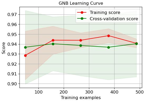
GNB:
logreg=modelss[‘GNB’]
skplt.estimators.plot_learning_curve(logreg, X, y,
cv=7, shuffle=True, scoring=”accuracy”,
n_jobs=-1, figsize=(6,4), title_fontsize=”large”, text_fontsize=”large”,
title=”GNB Learning Curve”);
plt.savefig(‘learningcurvegnb.png’, dpi=300, bbox_inches=’tight’)
QDA:
logreg=modelss[‘QDA’]
skplt.estimators.plot_learning_curve(logreg, X, y,
cv=7, shuffle=True, scoring=”accuracy”,
n_jobs=-1, figsize=(6,4), title_fontsize=”large”, text_fontsize=”large”,
title=”QDA Learning Curve”);
plt.savefig(‘learningcurveqda.png’, dpi=300, bbox_inches=’tight’)

It is clear that LR and GP learning curves perform the best in terms of training and CV scores when the number of training examples exceeds 450.
Confusion Matrix
Let’s look at the confusion matrix and the f1-score derived from the classification report
import seaborn as sns
from sklearn.metrics import classification_report, confusion_matrix
key=’Logistic Regression’
modelss[key].fit(X_train, y_train)
predictions = modelss[key].predict(X_test)
print(key)
print(classification_report(predictions, y_test))
Logistic Regression
              precision    recall  f1-score   support

           0       0.96      0.96      0.96        53
           1       0.98      0.98      0.98        90

    accuracy                           0.97       143
   macro avg       0.97      0.97      0.97       143
weighted avg       0.97      0.97      0.97       143
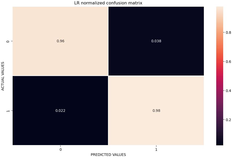
Let’s plot the LR normalized confusion matrix
confusion_matrix= confusion_matrix(y_test, predictions)
cm_normalized = confusion_matrix.astype(‘float’) / confusion_matrix.sum(axis=1)[:, np.newaxis]
fig, ax = plt.subplots(figsize=(12,7))
sns.heatmap(cm_normalized, annot=True, linewidths = 0.01, ax = ax)
ax.set_title(‘LR normalized confusion matrix’)
ax.set_xlabel(‘PREDICTED VALUES’)
ax.set_ylabel(‘ACTUAL VALUES’)
plt.savefig(‘normconfmatrixlr.png’, dpi=300, bbox_inches=’tight’)
Let’s calculate the accuracy, sensitivity and specificity derived from the above matrix
from sklearn.metrics import confusion_matrix
cm1 = confusion_matrix(y_test, predictions)
print(‘Confusion Matrix : \n’, cm1)
total1=sum(sum(cm1))
from confusion matrix calculate accuracy
accuracy1=(cm1[0,0]+cm1[1,1])/total1
print (‘Accuracy : ‘, accuracy1)
sensitivity1 = cm1[0,0]/(cm1[0,0]+cm1[0,1])
print(‘Sensitivity : ‘, sensitivity1 )
specificity1 = cm1[1,1]/(cm1[1,0]+cm1[1,1])
print(‘Specificity : ‘, specificity1)
Confusion Matrix :
 [[51  2]
 [ 2 88]]
Accuracy :  0.972027972027972
Sensitivity :  0.9622641509433962
Specificity :  0.9777777777777777
The higher the values of a test’s sensitivity and specificity (each out of 100%), the more accurate the test is in diagnosing BC.
Sensitivity: the ability of a test to correctly identify patients with BC.
Specificity: the ability of a test to correctly identify people without BC.
TP: the person has the disease and the test is positive.
TN: the person does not have the disease and the test is negative.
Let’s look at the SVC classifier
import seaborn as sns
from sklearn.metrics import classification_report, confusion_matrix
key=’Support Vector Machines’
modelss[key].fit(X_train, y_train)
predictions = modelss[key].predict(X_test)
print(key)
print(classification_report(predictions, y_test))
Support Vector Machines
              precision    recall  f1-score   support

           0       0.94      0.96      0.95        52
           1       0.98      0.97      0.97        91

    accuracy                           0.97       143
   macro avg       0.96      0.96      0.96       143
weighted avg       0.97      0.97      0.97       143
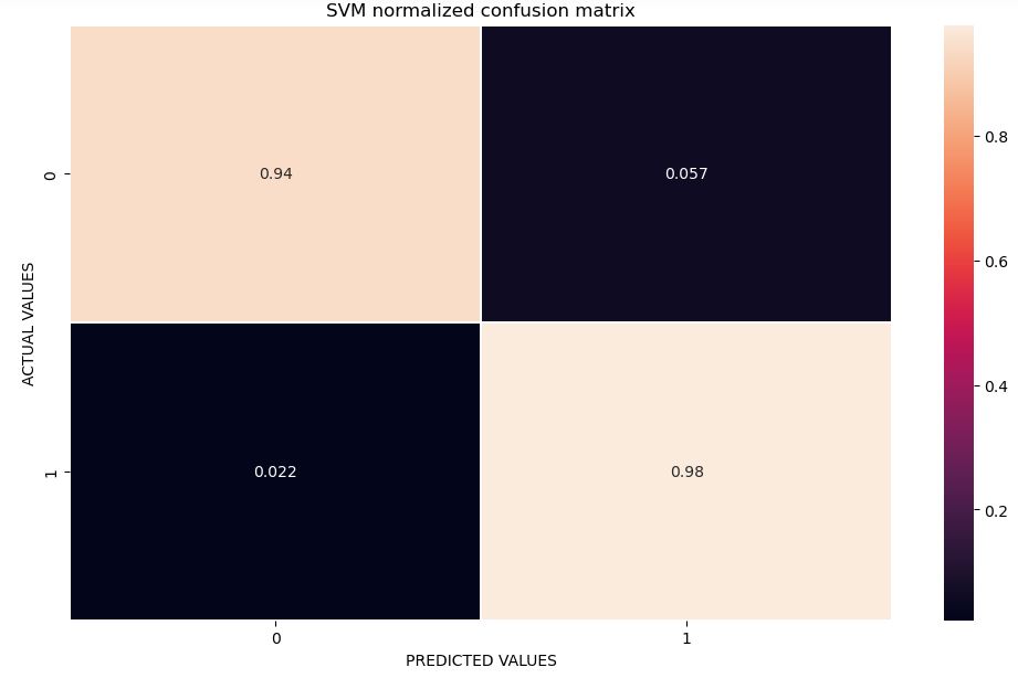
Let’s plot the SVM confusion matrix
confusion_matrix= confusion_matrix(y_test, predictions)
cm_normalized = confusion_matrix.astype(‘float’) / confusion_matrix.sum(axis=1)[:, np.newaxis]
fig, ax = plt.subplots(figsize=(12,7))
sns.heatmap(cm_normalized, annot=True, linewidths = 0.01, ax = ax)
ax.set_title(‘SVM normalized confusion matrix’)
ax.set_xlabel(‘PREDICTED VALUES’)
ax.set_ylabel(‘ACTUAL VALUES’)
plt.savefig(‘normconfmatrixsvm.png’, dpi=300, bbox_inches=’tight’)
Let’s calculate the SVM accuracy, sensitivity and specificity
from sklearn.metrics import confusion_matrix
cm1 = confusion_matrix(y_test, predictions)
print(‘Confusion Matrix : \n’, cm1)
total1=sum(sum(cm1))
from confusion matrix calculate accuracy
accuracy1=(cm1[0,0]+cm1[1,1])/total1
print (‘Accuracy : ‘, accuracy1)
sensitivity1 = cm1[0,0]/(cm1[0,0]+cm1[0,1])
print(‘Sensitivity : ‘, sensitivity1 )
specificity1 = cm1[1,1]/(cm1[1,0]+cm1[1,1])
print(‘Specificity : ‘, specificity1)
Confusion Matrix :
 [[50  3]
 [ 2 88]]
Accuracy :  0.965034965034965
Sensitivity :  0.9433962264150944
Specificity :  0.9777777777777777
* The specificity of a test is its ability to designate an individual who does not have a disease as negative.
* A highly specific test means that there are few false positive results.
* Sensitivity is the indicator on the ability of screening to find cancer in the detectable preclinical phase (DPCP).
* The ability is usually specified as to the screening test.
Accuracy-Precision-Recall-Cohen-F1 KPIs
Let’s look at the sklearn summary of model evaluation KPIs
from sklearn.metrics import accuracy_score, precision_score, recall_score
from sklearn.metrics import cohen_kappa_score
from sklearn.metrics import f1_score
accuracy, precision, recall, cohen, f1 = {}, {}, {}, {}, {}
for key in modelss.keys():
# Fit the classifier
modelss[key].fit(X_train, y_train)

# Make predictions
predictions = modelss[key].predict(X_test)

# Calculate metrics
accuracy[key] = accuracy_score(predictions, y_test)
precision[key] = precision_score(predictions, y_test)
recall[key] = recall_score(predictions, y_test)
cohen[key] = cohen_kappa_score(y_test, predictions)
f1[key]= f1_score(y_test, predictions)
import pandas as pd
df_model = pd.DataFrame(index=modelss.keys(), columns=[‘Accuracy’, ‘Precision’, ‘Recall’,’Cohen’])
df_model[‘Accuracy’] = accuracy.values()
df_model[‘Precision’] = precision.values()
df_model[‘Recall’] = recall.values()
df_model[‘Cohen’] = cohen.values()
df_model[‘f1’] = f1.values()
df_model

Let’s create the bar chart of this summary table
ax = df_model.plot.barh()
ax.legend(
ncol=len(models.keys()),
bbox_to_anchor=(0, 1),
loc=’lower left’,
prop={‘size’: 14}
)
plt.tight_layout()
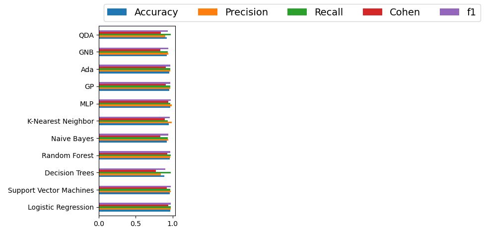
Cohen suggested the Kappa result be interpreted as follows: values ≤ 0 as indicating no agreement and 0.01–0.20 as none to slight, 0.21–0.40 as fair, 0.41– 0.60 as moderate, 0.61–0.80 as substantial, and 0.81–1.00 as almost perfect agreement.
Here is the summary of best performers based upon the above 5 KPIs
| Method | Accuracy | Precision | Recall | Cohen | F1 |
| QDA | * | * | 0.976 | * | * |
| GNB | * | * | * | * | * |
| Ada | * | * | * | * | * |
| GP | * | * | * | * | * |
| MLP | * | 0.988 | * | * | 0.978 |
| KNN | * | 0.988 | * | * | * |
| NB | * | * | * | * | * |
| RF | * | * | 0.977 | * | * |
| DT | * | * | * | * | * |
| SVM | * | * | * | * | * |
| LR | 0.972 | 0.977 | 0.977 | 0.94 | 0.977 |
It is clear that LR performs the best among these ML methods.
Other Performance Matrics
Let’s look at other available KPIs: matthews_corrcoef, log_loss, hinge_loss, jaccard_score, and fbeta_score
from sklearn.metrics import matthews_corrcoef
from sklearn.metrics import log_loss
from sklearn.metrics import hinge_loss
from sklearn.metrics import jaccard_score
from sklearn.metrics import fbeta_score
accuracy, precision, recall, cohen, f1 = {}, {}, {}, {}, {}
for key in modelss.keys():
# Fit the classifier
modelss[key].fit(X_train, y_train)

# Make predictions
predictions = modelss[key].predict(X_test)

# Calculate metrics
accuracy[key] = matthews_corrcoef(y_test,predictions)
precision[key] = log_loss(y_test,predictions)
recall[key] = hinge_loss(y_test,predictions)
cohen[key] = jaccard_score(y_test,predictions)
f1[key]= fbeta_score(y_test, predictions,beta=2)
import pandas as pd
df_model = pd.DataFrame(index=modelss.keys(), columns=[‘Mat’, ‘LL’, ‘HL’,’JS’,’FB’])
df_model[‘Mat’] = accuracy.values()
df_model[‘LL’] = precision.values()
df_model[‘HL’] = recall.values()
df_model[‘JS’] = cohen.values()
df_model[‘FB’] = f1.values()
df_model

Let’s create the bar chart of these attributes
ax = df_model.plot.barh()
ax.legend(
ncol=len(models.keys()),
bbox_to_anchor=(0, 1),
loc=’lower left’,
prop={‘size’: 14}
)
plt.tight_layout()
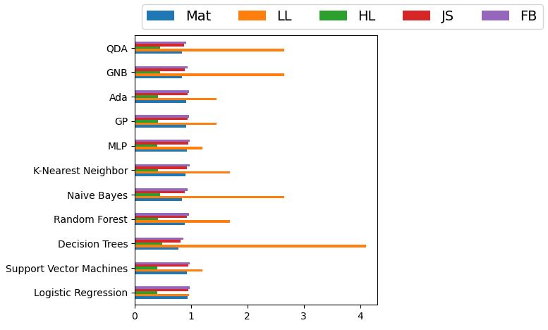
The Matthews correlation coefficient (MCC)
- A correlation of: Mat = 1 indicates perfect agreement, Mat = 0 is expected for a prediction no better than random, and Mat = -1 indicates total disagreement between prediction and observation.
- Log-loss is indicative of how close the prediction probability is to the corresponding actual/true value (0 or 1 in case of binary classification). The more the predicted probability diverges from the actual value, the higher is the log-loss value.
- Hinge-loss function is a scoring function used to evaluate how well a given boundary separates the training data.
- The Jaccard similarity index (sometimes called the Jaccard similarity coefficient) compares members for two sets to see which members are shared and which are distinct. It’s a measure of similarity for the two sets of data, with a range from 0% to 100%. The higher the percentage, the more similar the two populations.
- The F-beta score is the weighted harmonic mean of precision and recall, reaching its optimal value at 1 and its worst value at 0.
Conclusions
- A precise and reliable system is vital for the classification of cancerous sequences.
- ML/AI classifiers contribute much to the process of early prediction and diagnosis of BC.
- In this project, a comparative analysis of 12 ML BC binary classification models is implemented.
- We look at the following classifiers: LR, GB/GP, GNB, SVC, KNN, RF, ET, DT, MLP, QDA, Ada, and NB.
- Performance evaluation is conducted, and all classifiers are compared based on the available QC/QA metrics.
- The Linear Regression (LR) classifier of test data performs the best in terms of accuracy, precision, recall, f1-score, Cohen’s Kappa, MCC, log-loss, hinge-loss, the Jaccard similarity index, and fbeta-score.
- SVC returns the best average CV score of 0.973.
- Both SVC and LR return 2.2% FN, where the test result incorrectly indicates the absence of a condition.
- LR is the best performer in terms of FP=3.8%, where a test result incorrectly indicates the presence of a condition.
- LR and GP learning curves perform the best in terms of training and CV scores when the number of training examples exceeds 450.
- The best classification report
Logistic Regression
precision recall f1-score support
0 0.96 0.96 0.96 53
1 0.98 0.98 0.98 90
accuracy 0.97 143
macro avg 0.97 0.97 0.97 143
weighted avg 0.97 0.97 0.97 143
Explore More
Supervised ML/AI Breast Cancer Diagnostics (BCD) – The Power of HealthTech
HealthTech ML/AI Q3 ’22 Round-Up
A Comparative Analysis of Breast Cancer ML/AI Binary Classifications
A Comparison of Binary Classifiers for Enhanced ML/AI Breast Cancer Diagnostics – 1. Scikit-Plot
ML/AI Breast Cancer Diagnosis with 98% Confidence
ML/AI Breast Cancer Diagnostics – SciKit-Learn QC
Embed Socials
Infographic


Python BC ML code snippet 1:
Python BC ML code snippet 2:

Python BC ML code snippet 3:

AIHealth belongs to AIOps just like ML belongs to AI


Make a one-time donation
Make a monthly donation
Make a yearly donation
Choose an amount
Or enter a custom amount
Your contribution is appreciated.
Your contribution is appreciated.
Your contribution is appreciated.

Leave a comment