ML/AI Diamond Price Prediction with R

Inspired by the recent study, this post will cover an analysis of diamonds with R Studio. On the demand side, customers in the market for a less expensive, smaller diamond are probably more sensitive to price than more well-to-do buyers. Therefore, it makes a perfect sense to use a pre-trained ML/AI model to get an idea of whether you are overpaying.

Contents:

Preparation Phase

Let’s change our working directory to YOURPATH

setwd(“YOURPATH”)
getwd()

and install the following packages

type = “binary”
install.packages(“GGally”, type = “binary”)
install.packages(“tidymodels”, type = “binary”)
install.packages(“tictoc”, type = “binary”)
install.packages(“caTools”, type = “binary”)
install.packages(“xgboost”, type = “binary”)
install.packages(“e1071”, type = “binary”)
install.packages(“rpart”, type = “binary”)
install.packages(“randomForest”, type = “binary”)
install.packages(“Metrics”, type = “binary”)

We need a few libraries

library(‘tidyverse’)
library(‘GGally’)

library(caTools)
library(tictoc)

library(xgboost)

library(e1071)

library(rpart)

library(randomForest)

library(Metrics)

library(modelr)

and call the diamond data

data(diamonds)

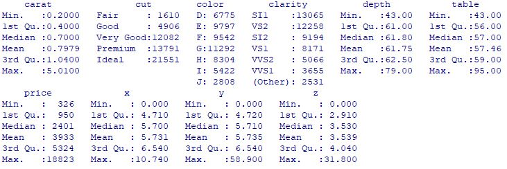
Here is the summary

summary(diamonds)

Exploratory Data Analysis (EDA)

Let’s look at the pair correlation plot

Let’s look at the Q-Q plot of log Price

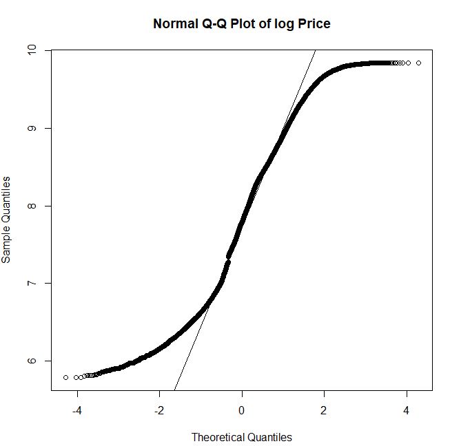
We can see that the multi-modal histogram of log Price does not follows the normal distribution

hist_norm <- ggplot(diamonds, aes(log(price))) +
geom_histogram(aes(y = ..density..), colour = “black”, fill = ‘yellow’, bins = 55) +
stat_function(fun = dnorm, args = list(mean = mean(log(diamonds$price)), sd = sd(log(diamonds$price))))
hist_norm

Let’s consider log Price as the target variable and split the input data with SplitRatio = 0.7

split = sample.split(diamonds$log_price, SplitRatio = 0.7)
diamonds_train = subset(diamonds, split == TRUE)
diamonds_test = subset(diamonds, split == FALSE)

Let’s prepare the data for ML

diamonds_train <- diamonds_train %>%
mutate_at(c(‘table’, ‘depth’), ~(scale(.) %>% as.vector))
diamonds_test <- diamonds_test %>%
mutate_at(c(‘table’, ‘depth’), ~(scale(.) %>% as.vector))

Training Model

Let’s call the lm() function to fit linear models

mlm <- lm(log_price ~ carat + color + cut + clarity + table + depth, diamonds_train)
mlm
summary(mlm)

mlm: 0.04 sec elapsed

lm summary: residuals, coefficients, signif. codes, residual standard error 0.345, R2=0.88, p-value 2.2.e-16, and F-statistic 1.51e+4.

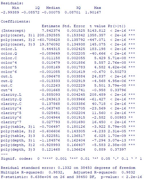
Let’s call the 3rd order polynomial function lm()

poly <- lm(log_price ~ poly(carat,3) + color + cut + clarity + poly(table,3) + poly(depth,3), diamonds_train)
poly
summary(poly)

lm poly 3 summary: residuals, coefficients, signif. codes, residual standard error 0.1332, R2=0.98, p-value 2.2.e-16, and F-statistic 8.64e+4.

Let’s apply the XGBoost algorithm to both training and test data

diamonds_train_xgb <- diamonds_train %>%
mutate_if(is.factor, as.numeric)
diamonds_test_xgb <- diamonds_test %>%
mutate_if(is.factor, as.numeric)

xgb <- xgboost(data = as.matrix(diamonds_train_xgb[-7]), label = diamonds_train_xgb$log_price, nrounds = 6166, verbose = 0)

xgb

xgb_pred = predict(xgb, as.matrix(diamonds_test_xgb[-7]))

y_actual <- diamonds_test_xgb$log_price
y_predicted <- xgb_pred

test <- data.frame(cbind(y_actual, y_predicted))

let’s look at the test actual-predicted data cross-plot

xgb_scatter <- ggplot(test, aes(10y_actual, 10y_predicted)) + geom_point(colour = ‘black’, alpha = 0.3) + geom_smooth(method = lm)
xgb_scatter

XGBoost test actual-predicted data cross-plot

Let’s apply the SVM algorithm to both training and test data using kernel = ‘radial’

svr <- svm(formula = log_price ~ .,
data = diamonds_train,
type = ‘eps-regression’,
kernel = ‘radial’)

Call:
svm(formula = log_price ~ ., data = diamonds_train, type = “eps-regression”, kernel = “radial”)

Parameters:
SVM-Type: eps-regression
SVM-Kernel: radial
cost: 1
gamma: 0.04761905
epsilon: 0.1

Number of Support Vectors: 13718

Let’s switch to the Decision Tree algorithm

tree <- rpart(formula = log_price ~ .,
data = diamonds_train,
method = ‘anova’,
model = TRUE)
tree

Let’s consider the Random Forest approach

rf <- randomForest(log_price ~ .,
data = diamonds_train,
ntree = 500)
rf

Call:
randomForest(formula = log_price ~ ., data = diamonds_train, ntree = 500)
Type of random forest: regression
Number of trees: 500
No. of variables tried at each split: 2

      Mean of squared residuals: 0.01172975
                % Var explained: 98.89

Model Performance

Let’s make predictions and compare model performance

mlm_pred <- predict(mlm, diamonds_test)
poly_pred <- predict(poly, diamonds_test)
svr_pred <- predict(svr, diamonds_test)
tree_pred <- predict(tree, diamonds_test)
rf_pred <- predict(rf, diamonds_test)
xgb_pred <- predict(xgb, as.matrix(diamonds_test_xgb[-7]))

xgb_resid <- diamonds_test_xgb$log_price – xgb_pred

resid <- diamonds_test %>%
spread_residuals(mlm, poly, svr, tree, rf) %>%
select(mlm, poly, svr, tree, rf) %>%
rename_with( ~ paste0(.x, ‘_resid’)) %>%
cbind(xgb_resid)

predictions <- diamonds_test %>%
select(log_price) %>%
cbind(mlm_pred) %>%
cbind(poly_pred) %>%
cbind(svr_pred) %>%
cbind(tree_pred) %>%
cbind(rf_pred) %>%
cbind(xgb_pred) %>%
cbind(resid)

mean_log_price <- mean(diamonds_test$log_price)
tss = sum((diamonds_test_xgb$log_price – mean_log_price)^2 )

square <- function(x) {x**2}
r2 <- function(x) {1 – x/tss}

r2_df <- resid %>%
mutate_all(square) %>%
summarize_all(sum) %>%
mutate_all(r2) %>%
gather(key = ‘model’, value = ‘r2’) %>%
mutate(model = str_replace(model, ‘_resid’, ”))
r2_df

model r2
1 mlm 0.8916784
2 poly 0.9813779
3 svr 0.9862363
4 tree 0.9103298
5 rf 0.9882366
6 xgb 0.9860271

xgb_rmse = sqrt(mean(residuals^2))

Let’s look at the model performance plot

r2_plot <- ggplot(r2_df, aes(x = model, y = r2, colour = model, fill = model)) + geom_bar(stat = ‘identity’)
r2_plot + ggtitle(‘R-squared Values for each Model’) + coord_cartesian(ylim = c(0.75, 1))

Model performance in terms of R-squared values

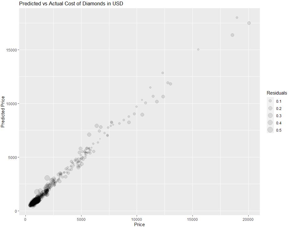
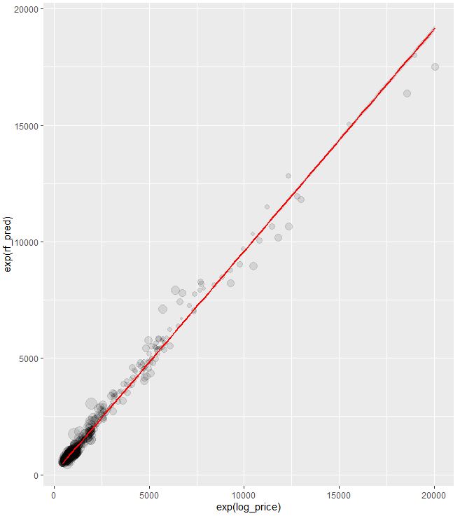
Let’s look at the predicted vs actual price of the test data

diamonds_test_sample <- diamonds_test %>%
left_join(predictions, by = ‘log_price’) %>%
slice_sample(n = 1000)
ggplot(diamonds_test_sample, aes(x = exp(log_price), y = exp(rf_pred), size = abs(rf_resid))) +
geom_point(alpha = 0.1) + labs(title = ‘Predicted vs Actual Cost of Diamonds in USD’, x = ‘Price’, y = ‘Predicted Price’, size = ‘Residuals’)

Predicted vs actual price in USD of the test data

Linear fit: Predicted vs actual price in USD of the test data — Linear fit (red line): Predicted vs actual price in USD of the test data

Key Takeaways

The Random Forest model performed best according to the R2 value.

The critical factor driving price is the size or the carat weight of the diamond.

Recall that we applied the log transformation to our long-tailed dollar variable before using it in regression.

You can use the above pre-trained model to get a sense of whether you are overpaying for establishing a lasting business relationship with a jeweler you can trust.