
Gulf states to gain $1.3 trillion in additional oil revenue by 2026: IMF.
- The gains, due to high oil prices, are expected to provide ‘firepower’ to the region’s sovereign wealth funds (SWFs), one of the largest in the world.
- Most of the oil and gas exporters in the region have large SWFs and have been using them to use the windfall in further investments. Some of these are Saudi Arabia’s Public Investment Fund, the Qatar Investment Authority, Abu Dhabi Investment Authority, Mubadala, and ADQ.
- Saudi’s PIF is chaired by crown prince Mohammed bin Salman. It has invested over $620 billion in total. Out of these, $7.5 billion alone were invested in US stocks during the second quarter, when the share prices were relatively low. PIF bought stocks of Amazon. PayPal, and BlackRock, among others, according to the report.
Let’s discuss the basics of sourcing oil market price data for free online. Webscraping in R is a technique to retrieve large amounts of data from the Internet.
We’ll be scraping data on Gulf’s oil prices from the Oil Price website and converting it into a usable format.
Let’s install the R version 4.1.2 (2021-11-01) of the R Foundation for Statistical Computing. It is available within the Anaconda IDE.
Let’s set up the working directory YOURPATH
setwd(“YOURPATH”)
and install the following packages via CRAN
type = “binary”
install.packages(“rvest”, type = “binary”)
install.packages(“tidyverse”, type = “binary”)
install.packages(“ggpubr”, type = “binary”)
We need the following libraries
library(rvest)
library(tidyverse)
library(ggplot2)
library(ggpubr)
The relevant R webscraping script is given by
url <- “https://oilprice.com/oil-price-charts” webpage <- read_html(url) print(webpage) value <- webpage %>%
html_nodes( css = “.last_price”) %>%
html_text()
name <- webpage %>%
html_nodes(., css = “td:nth-child(2)”) %>%
html_text() %>%
.[c(41:72, 74, 76:77, 79, 81:82, 84:85, 87:89, 91, 94:96, 98:99, 101:103, 105:107, 109:112, 114:116, 118:120, 122:124,
126:128, 130:131, 133, 135:142, 145:160, 162:164, 166:167, 169:170, 172, 174,
176:178, 180:182, 184:186, 188:189, 191, 193:196, 198:199, 201:213)]
name1=append (name, NA, after=138)
name2=append (name1, NA, after=139)
name3=append (name2, NA, after=140)
prices <- tibble(name = name3,
last_price = value)
name10=head(name3,n=10)
value10=head(value,n=10)
prices10 <- tibble(namex = name10,
last_pricex = value10)
tabprices10=table(prices10$namex, prices10$last_pricex)
Let’s create the basic scatter plot
df <- data.frame(brand=prices10$namex,
price=prices10$last_pricex)
print(df)
brand price
1 Al Shaheen – Qatar 88.77
2 Iraq 95.02
3 Basrah Heavy 96.07
4 Basrah Medium 8.361
5 Saudi Arabia 3.617
6 Arab Extra Light 86.19
7 Arab Heavy 95.28
8 Arab Medium 66.49
9 Nigeria 93.53
10 Brass River 82.50
ggbarplot(df, “brand”, “price”,
fill = “steelblue”, color = “steelblue”,
label = TRUE, lab.pos = “in”, lab.col = “white”)
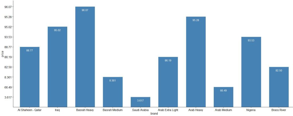
This chart is crucial for competitive pricing. In order to keep prices of your products competitive and attractive, you need to monitor and keep track of prices set by your competitors. If you know what your competitors’ pricing strategy is, you can accordingly align your pricing strategy to get an edge over them.
Explore More
Webscraping in R – IMDb ETL Showcase
Firsthand Data Visualization in R: Examples
Tutorial: Web Scraping in R with rvest
Web Scrape Text from ANY Website – Web Scraping in R (Part 1)


Leave a comment