
Featured Photo by Mike Newbry on Unsplash
Contents:
- Introduction
- Canadian Dataset
- ML/AI Workflow
- E2E Use-Case
- ML Performance Plots
- ML Classification Reports
- Summary
- Conclusions
- References
Introduction
Wildfire is a widespread and critical element of the Earth’s system. Wildfires can result in significant impacts to humans, either directly through loss of life and destruction to communities or indirectly through smoke exposure. As the climate warms, we are seeing increasing impacts from wildfire.
Consequently, billions of dollars are spent every year on the Fire Technology (FireTech) development to support wildfire science, management, and disaster mitigation. Understanding and better predicting wildfires is therefore crucial in several important areas of wildfire management, including emergency response, ecosystem management, land-use planning, and climate adaptation to name a few [1-2].
Remote sensing (RS) can play an enormous role in FireTech for preventing and planning for wildfires. While some aspects require more advanced RS skills, many can be performed with the guided tools such as Machine Learning (ML) and Artificial Intelligence (AI) algorithms [1-7].
The goal of this case study is to apply the depolyed FireTech ML/AI applications [4,5] to the RS data acquired in Canada [1]. Different binary classifiers will be adopted. The predicted results will then be compared with the actual occurrence of forest fires for validation and performance QC.
Canadian Dataset
The input dataset was created based on RS data to predict and monitor the occurrence of wildfires [1]. It contains data related to the state of crops (NDVI: Normalized Difference Vegetation Index), meteorological conditions (LST: Land Surface Temperature) as well as the fire indicator “Thermal Anomalies” (TA). The fourth column represents the corresponding class (fire or no_fire). The data were downloaded from the official website of NASA‘s Land Processes Distributed Active Archive Center (LP DAAC), and then we preprocessed them using multiple preprocessing techniques to remove noises and correct inconsistencies, and finally extracting useful information.
The study area is composed of multiple zones located in the center of Canada. The surface of this area is approximately 2 million hectares. These zones differ in their size, burn period, date of burn and extent. We have chosen to apply the experiment in a big region of Canada’s forests because it is known for its high rate of wildfires and also for the availability of fire information (start and end fire date, cause of fire and the surface of the burned area in hectares), these information were acquired from The Canadian Wild-land Fire Information System (CWFIS) which creates daily fire weather and fire behavior maps year-round and hot spot maps throughout the forest fire season
ML/AI Workflow
The entire Python-3 workflow implemented in Jupyter/Anaconda IDE is as follows:
- Import/install relevant libraries
- Read/download input dataset
- Exploratory Data Analysis (EDA)
- ML Data Preparation/Scaling/Balancing
- Train Different Binary Classifiers
- Compare Full Classification Reports
- Hyperparameter Optimization (HPO)
- Predict Test Data using Trained Models
- Final Performance QC Visualization
- Save Training Models for Future Use.
E2E Use-Case
Import Libraries
Let’s set the working directory YOURPATH
import os
os. getcwd()
os.chdir(‘YOURPATH’)
and import the libraries
import numpy as np
import pandas as pd
import matplotlib.pyplot as plt
plt.style.use(‘seaborn’)
import seaborn as sns
from sklearn.preprocessing import LabelEncoder, StandardScaler, MinMaxScaler
from sklearn.model_selection import train_test_split
from sklearn.metrics import r2_score
import tensorflow as tensorflow
from keras.models import Sequential
from keras.layers import Dense, Dropout
from tensorflow import keras
from tensorflow.keras import layers
from tensorflow.keras.optimizers import SGD
from tensorflow.keras.utils import to_categorical
from keras.callbacks import EarlyStopping
from keras.callbacks import ModelCheckpoint
from keras.utils.vis_utils import plot_model
import warnings
import time
%matplotlib inline
warnings.filterwarnings(‘ignore’)
sns.set_style(“darkgrid”)
Read Input Data
Let’s read the input dataset
data = pd.read_csv(‘WildFires_DataSet.csv’)
data.head(5)
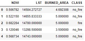
Here, NDVI = Normalized Difference Vegetation Index, LST = Land Surface Temperature, BURNED_AREA = TA (see above), and CLASS represents the binary class (fire or no_fire).
Exploratory Data Analysis
The dataset shape is
print(data.shape)
(1713, 4)
There are 1713 rows (measurements) and 4 attributes/features.
We see that there are no null values
data.info(verbose=True)
<class 'pandas.core.frame.DataFrame'>
RangeIndex: 1713 entries, 0 to 1712
Data columns (total 4 columns):
 #   Column       Non-Null Count  Dtype
---  ------       --------------  -----
 0   NDVI         1713 non-null   float64
 1   LST          1713 non-null   float64
 2   BURNED_AREA  1713 non-null   float64
 3   CLASS        1713 non-null   object
dtypes: float64(3), object(1)
memory usage: 53.7+ KB
Let’s drop duplicates
df=data.drop_duplicates()
df.info(verbose=True)
<class 'pandas.core.frame.DataFrame'>
Int64Index: 1438 entries, 0 to 1712
Data columns (total 4 columns):
 #   Column       Non-Null Count  Dtype
---  ------       --------------  -----
 0   NDVI         1438 non-null   float64
 1   LST          1438 non-null   float64
 2   BURNED_AREA  1438 non-null   float64
 3   CLASS        1438 non-null   object
dtypes: float64(3), object(1)
memory usage: 56.2+ KB
So, we have removed 275 duplicates.
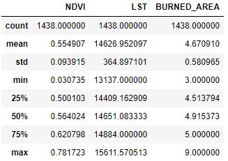
Let’s check statistical information about numerical fields
data_train=df
data_train.describe()
Selecting rows based on condition
fire_df = df[df[‘CLASS’] == “fire”]
print(fire_df.shape)
(329, 4)
nofire_df = df[df[‘CLASS’] == “no_fire”]
print(nofire_df.shape)
(1109, 4)
Let’s compare them to check the class imbalance of target variable CLASS in
data_train[‘CLASS’].value_counts(normalize=True)
no_fire    0.77121
fire       0.22879
Name: CLASS, dtype: float64
Let’s check null/missing values
df.info()
<class 'pandas.core.frame.DataFrame'>
Int64Index: 1438 entries, 0 to 1712
Data columns (total 4 columns):
 #   Column       Non-Null Count  Dtype
---  ------       --------------  -----
 0   NDVI         1438 non-null   float64
 1   LST          1438 non-null   float64
 2   BURNED_AREA  1438 non-null   float64
 3   CLASS        1438 non-null   object
dtypes: float64(3), object(1)
memory usage: 56.2+ KB
df.isnull().sum().sort_values()
NDVI           0
LST            0
BURNED_AREA    0
CLASS          0
dtype: int64
Let’s plot the target variable
plt.figure(figsize= (8,4))
df[“CLASS”].value_counts(normalize = True).plot.bar()
plt.title(“Bar chart analysing CLASS variable\n”, fontdict={‘fontsize’: 20, ‘fontweight’ : 5, ‘color’ : ‘Green’})
plt.show()
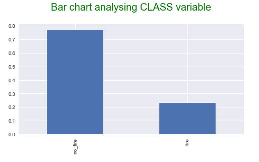
This plot shows that this is an imbalanced classification problem where the distribution of CLASS is uneven by a small amount in the training dataset.
Let’s look at the pairplot of other variables
sns.pairplot(df)

The histogram of BURNED_AREA is
data[‘BURNED_AREA’].nunique()
sns.displot(data[‘BURNED_AREA’])

We can see that BURNED_AREA ~ 3-5.
The histogram of NDVI is
data[‘NDVI’].nunique()
sns.displot(data[‘NDVI’])

It appears that NDVI ~ 0.4-0.7.
The histogram of LST is
data[‘LST’].nunique()
sns.displot(data[‘LST’])

It is clear that LST ~ 13500-15500.
The scatter plot NDVI vs BURNED_AREA is
plt.figure(figsize= [10,6])
plt.scatter(data[“NDVI”], data[“BURNED_AREA”], alpha = 0.5)
plt.title(“Scatter plot analysing NDVI vs BURNED_AREA\n”, fontdict={‘fontsize’: 20, ‘fontweight’ : 5, ‘color’ : ‘Green’})
plt.xlabel(“NDVI”, fontdict={‘fontsize’: 12, ‘fontweight’ : 5, ‘color’ : ‘Black’})
plt.ylabel(“BURNED_AREA”, fontdict={‘fontsize’: 12, ‘fontweight’ : 5, ‘color’ : ‘Black’} )
plt.show()

This plot illustrates subzero correlation between NDVI and BURNED_AREA.
We can also plot the 3×3 correlation matrix
import seaborn as sns
sns_heat=sns.heatmap(df.corr(), annot=True)
sns_heat.figure.savefig(“snscorrheatmap.png”)
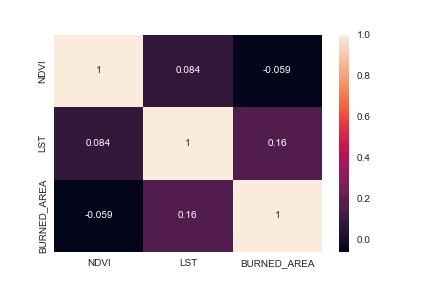
So I draw a pairplot/heatmap from the feature correlations of a dataset and see a set of features that bears weak/subzero correlations both with:
- every other feature and
- also with the target/label.
Let’s look at the following boxplots
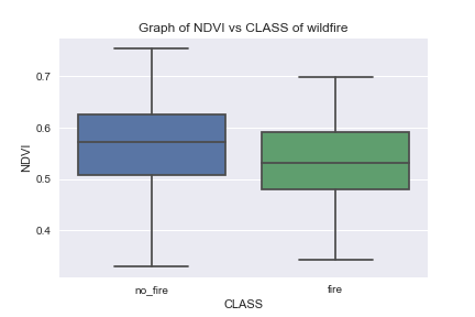
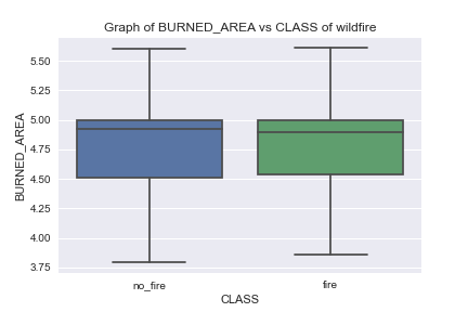
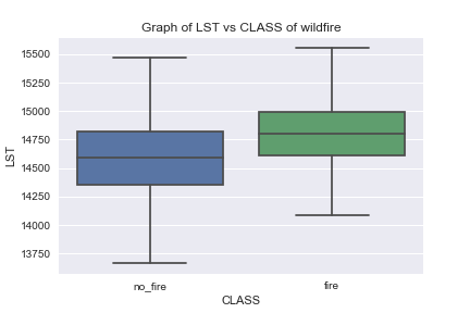
We can see the least overlap of LST-CLASS boxplots compared to BURNED_AREA- and NDVI-CLASS boxplots.
Let’s split the target and other features
X = df[[‘NDVI’, ‘LST’ , ‘BURNED_AREA’]]
Y=df[‘CLASS’]
Let’s perform Y encoding using LabelEncoder
from sklearn.preprocessing import LabelEncoder
labelencoder_y = LabelEncoder()
Y= labelencoder_y.fit_transform(Y)
print(labelencoder_y.fit_transform(Y))
[1 1 0 ... 1 0 0]
Let’s split the input dataset into 80% training and 20% testing data
from sklearn.model_selection import train_test_split
X_train, X_test, Y_train, Y_test= train_test_split(X,Y,test_size=0.20, random_state=1)
Let’s perform data scaling using RobustScaler
from sklearn.preprocessing import RobustScaler
sc = RobustScaler()
X_train = sc.fit_transform(X_train)
X_test = sc.transform(X_test)
y_train=Y_train
Training Model
Let’s define a function which trains models
def models(X_train,y_train):
#Using Logistic Regression
from sklearn.linear_model import LogisticRegression
log = LogisticRegression(random_state = 0)
log.fit(X_train, y_train)
#Using SVC linear
from sklearn.svm import SVC
svc_lin = SVC(kernel = ‘linear’, random_state = 0)
svc_lin.fit(X_train, y_train)
#Using SVC rbf
from sklearn.svm import SVC
svc_rbf = SVC(kernel = ‘rbf’, random_state = 0)
svc_rbf.fit(X_train, y_train)
#Using DecisionTreeClassifier
from sklearn.tree import DecisionTreeClassifier
tree = DecisionTreeClassifier(criterion = ‘entropy’, random_state = 0)
tree.fit(X_train, y_train)
#Using Random Forest Classifier
from sklearn.ensemble import RandomForestClassifier
forest = RandomForestClassifier(n_estimators = 10, criterion = ‘entropy’, random_state = 0)
forest.fit(X_train, y_train)
#print model accuracy on the training data.
print(‘[0]Logistic Regression Training Accuracy:’, log.score(X_train, y_train))
print(‘[1]Support Vector Machine (Linear Classifier) Training Accuracy:’, svc_lin.score(X_train, y_train))
print(‘[2]Support Vector Machine (RBF Classifier) Training Accuracy:’, svc_rbf.score(X_train, y_train))
print(‘[3]Decision Tree Classifier Training Accuracy:’, tree.score(X_train, y_train))
print(‘[4]Random Forest Classifier Training Accuracy:’, forest.score(X_train, y_train))
return log, svc_lin, svc_rbf, tree, forest
and get the training results using this function
model = models(X_train,y_train)
[0]Logistic Regression Training Accuracy: 0.7747826086956522
[1]Support Vector Machine (Linear Classifier) Training Accuracy: 0.7695652173913043
[2]Support Vector Machine (RBF Classifier) Training Accuracy: 0.7834782608695652
[3]Decision Tree Classifier Training Accuracy: 1.0
[4]Random Forest Classifier Training Accuracy: 0.9878260869565217
We can see that model 4 yields the best training accuracy of 98%, whereas the 100% accuracy of model 3 signifies data overfitting.
Testing Model
Let’s predict our test data while calculating the confusion matrix
y_test=Y_test
from sklearn.metrics import confusion_matrix
for i in range(len(model)):
cm = confusion_matrix(y_test, model[i].predict(X_test))
TN = cm[0][0]
TP = cm[1][1]
FN = cm[1][0]
FP = cm[0][1]
print(cm)
print(‘Model[{}] Testing Accuracy = “{}”‘.format(i, (TP + TN) / (TP + TN + FN + FP)))
[[  7  57]
 [  8 216]]
Model[0] Testing Accuracy = "0.7743055555555556"
[[  0  64]
 [  0 224]]
Model[1] Testing Accuracy = "0.7777777777777778"
[[  2  62]
 [  2 222]]
Model[2] Testing Accuracy = "0.7777777777777778"
[[ 25  39]
 [ 33 191]]
Model[3] Testing Accuracy = "0.75"
[[ 20  44]
 [ 21 203]]
Model[4] Testing Accuracy = "0.7743055555555556"
We can see that the prediction accuracy of model 4 is about 77%.
Let’s create the classification report
from sklearn.metrics import classification_report
from sklearn.metrics import accuracy_score
for i in range(len(model)):
print(‘Model ‘,i)
#Check precision, recall, f1-score
print(classification_report(y_test, model[i].predict(X_test)))
#Another way to get the models accuracy on the test data
print(accuracy_score(y_test, model[i].predict(X_test)))
print()#Print a new line
Model  0
              precision    recall  f1-score   support

           0       0.47      0.11      0.18        64
           1       0.79      0.96      0.87       224

    accuracy                           0.77       288
   macro avg       0.63      0.54      0.52       288
weighted avg       0.72      0.77      0.72       288

0.7743055555555556

Model  1
              precision    recall  f1-score   support

           0       0.00      0.00      0.00        64
           1       0.78      1.00      0.88       224

    accuracy                           0.78       288
   macro avg       0.39      0.50      0.44       288
weighted avg       0.60      0.78      0.68       288

0.7777777777777778

Model  2
              precision    recall  f1-score   support

           0       0.50      0.03      0.06        64
           1       0.78      0.99      0.87       224

    accuracy                           0.78       288
   macro avg       0.64      0.51      0.47       288
weighted avg       0.72      0.78      0.69       288

0.7777777777777778

Model  3
              precision    recall  f1-score   support

           0       0.43      0.39      0.41        64
           1       0.83      0.85      0.84       224

    accuracy                           0.75       288
   macro avg       0.63      0.62      0.63       288
weighted avg       0.74      0.75      0.75       288

0.75

Model  4
              precision    recall  f1-score   support

           0       0.49      0.31      0.38        64
           1       0.82      0.91      0.86       224

    accuracy                           0.77       288
   macro avg       0.65      0.61      0.62       288
weighted avg       0.75      0.77      0.76       288

0.7743055555555556
Recall that the f1-score can range from 0 to 1, with 1 representing a model that perfectly classifies each observation into the correct class and 0 representing a model that is unable to classify any observation into the correct class.
It is given by
f1-score = 2 * (Precision * Recall) / (Precision + Recall)
where:
- Precision: Correct positive predictions relative to total positive predictions
- Recall: Correct positive predictions relative to total actual positives
results show that the f1-score of 0.84-0.88 is close to 1.0 representing a model that perfectly classifies test observations into the target CLASS=1 (fire).
Hyperparameter Optimization (HPO)
Let’s apply HPO using GridSearchCV
from sklearn.linear_model import LogisticRegression
from sklearn.model_selection import GridSearchCV
from sklearn import linear_model
Let’s consider linear logistic regression
logistic = linear_model.LogisticRegression()
and make the scoring function with beta = 2
from sklearn.metrics import fbeta_score, make_scorer
ftwo_scorer = make_scorer(fbeta_score, beta=2)
Let’s create the regularization penalty space
penalty = [‘none’, ‘l2’]
and hyperparameters
C = np.logspace(0, 4, 10)
hyperparameters = dict(C=C, penalty=penalty)
Let’s run grid search with the 5-fold cross validation
clf = GridSearchCV(logistic, hyperparameters, cv=5, scoring=ftwo_scorer, verbose=0)
and fit the training set
best_model = clf.fit(X_train, y_train)
View best hyperparameters
print(‘Best Penalty:’, best_model.best_estimator_.get_params()[‘penalty’])
print(‘Best C:’, best_model.best_estimator_.get_params()[‘C’])
Best Penalty: l2
Best C: 2.7825594022071245
Let’s make test predictions
predictions = best_model.predict(X_test)
print(“Accuracy score %f” % accuracy_score(y_test, predictions))
print(classification_report(y_test, predictions))
print(confusion_matrix(y_test, predictions))
Accuracy score 0.774306
              precision    recall  f1-score   support

           0       0.47      0.11      0.18        64
           1       0.79      0.96      0.87       224

    accuracy                           0.77       288
   macro avg       0.63      0.54      0.52       288
weighted avg       0.72      0.77      0.72       288

[[  7  57]
 [  8 216]]
Let’s create the score
y_scores = best_model.predict_proba(X_test)[:, 1]
print(y_scores)
[0.79745919 0.77771936 0.54059685 0.87961689 0.66450793 0.36927774
 0.60238209 0.87317147 0.71121616 0.56358383 0.89626439 0.85553933
 0.73748319 0.81283213 0.83050708 0.76913056 0.94599292 0.72874697
 0.68789026 0.68294327 0.7584037  0.40763254 0.83691165 0.95716624
 0.76167625 0.81272648 0.72029233 0.86360586 0.61850486 0.67717831
 0.2847362  0.81108591 0.84943916 0.85264938 0.81796591 0.74797941
 0.93641704 0.45521339 0.81596063 0.47823083 0.87812436 0.76108541
 0.69501061 0.90666732 0.66302205 0.92545223 0.88600113 0.75850962
 0.79424947 0.5690601  0.37354364 0.62210546 0.60449876 0.62218612
 0.87522281 0.73177788 0.90970642 0.88695691 0.6046835  0.64995969
etc.
]
Y_test= labelencoder_y.fit_transform(Y_test)
print(labelencoder_y.fit_transform(Y_test))
[1 1 0 0 0 0 1 1 0 1 1 0 1 1 1 1 1 1 0 1 1 1 1 1 1 1 1 1 0 1 1 1 0 1 1 1 1
 0 1 1 0 1 1 1 1 0 1 1 1 0 0 1 1 1 1 1 0 1 1 1 1 0 1 1 0 1 1 0 0 1 1 1 1 1
 1 0 1 1 1 1 1 0 1 0 1 1 1 1 0 1 1 1 1 1 1 1 1 0 0 0 1 0 1 1 1 1 0 1 1 1 1
 1 0 0 1 0 1 1 1 0 1 1 1 1 0 0 0 1 1 1 0 1 1 1 1 1 1 1 1 1 0 1 1 1 0 1 1 1
 1 1 1 1 1 1 1 1 0 1 1 1 1 1 1 1 1 1 0 1 1 1 1 1 1 1 1 0 1 1 1 1 1 1 0 1 1
 1 0 1 1 1 1 1 0 1 0 0 1 1 0 1 1 1 1 1 0 1 1 1 1 1 1 0 0 1 1 1 1 1 1 1 1 1
 1 1 0 1 1 0 1 1 1 1 1 0 0 1 1 1 1 1 1 0 1 1 1 1 0 0 1 1 1 1 1 1 1 1 1 1 1
 0 0 1 0 1 0 1 1 0 1 1 1 1 1 1 1 1 1 1 1 1 0 1 1 1 1 1 0 1]
Let’s call the precision_recall_curve function
from sklearn.metrics import precision_recall_curve
p, r, thresholds = precision_recall_curve(Y_test, y_scores)
and define the function
def precision_recall_threshold(p, r, thresholds, t=0.5):
y_pred_adj = adjusted_classes(y_scores, t)
print(pd.DataFrame(confusion_matrix(Y_test, y_pred_adj),
columns=[‘pred_neg’, ‘pred_pos’],
index=[‘neg’, ‘pos’]))
print(classification_report(Y_test, y_pred_adj))
and call this function
precision_recall_threshold(p, r, thresholds, 0.42)
 pred_neg  pred_pos
neg         3        61
pos         3       221
              precision    recall  f1-score   support

           0       0.50      0.05      0.09        64
           1       0.78      0.99      0.87       224

    accuracy                           0.78       288
   macro avg       0.64      0.52      0.48       288
weighted avg       0.72      0.78      0.70       288
Let’s plot precision as a function of the decision threshold
plt.figure(figsize=(12,10))
plt.plot(thresholds, p[:-1])
plt.xlabel(‘threshold’,fontsize=18)
plt.ylabel(‘precision’,fontsize=18)
plt.title(‘Precision as a function of the decision threshold’,fontsize=18)
plt.xticks(fontsize=16)
plt.yticks(fontsize=16)
plt.grid(True)
plt.savefig(‘precisionthreshold_class.png’)

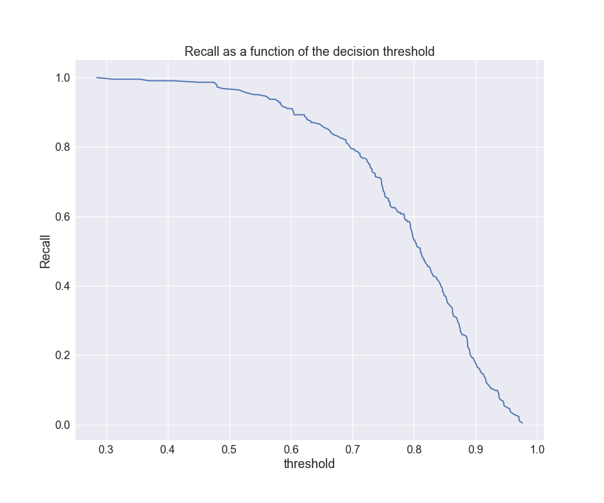
Let’s plot recall as a function of the decision threshold
plt.figure(figsize=(12,10))
plt.plot(thresholds, r[:-1])
plt.xlabel(‘threshold’,fontsize=18)
plt.ylabel(‘Recall’,fontsize=18)
plt.title(‘Recall as a function of the decision threshold’,fontsize=18)
plt.xticks(fontsize=16)
plt.yticks(fontsize=16)
plt.grid(True)
plt.savefig(‘recallthreshold_class.png’)
Let’s plot the ROC curve
from sklearn import metrics
from sklearn.metrics import roc_curve
#Compute predicted probabilities: y_pred_prob
y_pred_prob = best_model.predict_proba(X_test)[:,1]
#Generate ROC curve values: fpr, tpr, thresholds
fpr, tpr, thresholds = roc_curve(Y_test, y_pred_prob)
print(metrics.auc(fpr, tpr))
plt.figure(figsize=(12,10))
#Plot ROC curve
#plt.plot([0, 1], [0, 1], ‘k — ‘)
plt.plot(fpr, tpr)
plt.xlabel(‘False Positive Rate’,fontsize=18)
plt.ylabel(‘True Positive Rate’,fontsize=18)
plt.title(‘ROC Curve for Logistic Regression’,fontsize=18)
plt.xticks(fontsize=16)
plt.yticks(fontsize=16)
plt.savefig(‘ROCcurve.png’)
#plt.show()

and print the ROC score for Logistic Regression + HPO
0.6778041294642856
ML Performance Plots
Let’s invoke Scikit-Plot for Visualizing ML Algorithm Results & Performance:
import scikitplot as skplt
import sklearn
from sklearn.datasets import load_digits, load_boston, load_breast_cancer
from sklearn.model_selection import train_test_split
from sklearn.ensemble import RandomForestClassifier, RandomForestRegressor, GradientBoostingClassifier, ExtraTreesClassifier
from sklearn.linear_model import LinearRegression, LogisticRegression
from sklearn.cluster import KMeans
from sklearn.decomposition import PCA
import matplotlib.pyplot as plt
import sys
import warnings
warnings.filterwarnings(“ignore”)
print(“Scikit Plot Version : “, skplt.version)
print(“Scikit Learn Version : “, sklearn.version)
print(“Python Version : “, sys.version)
%matplotlib inline
Scikit Plot Version :  0.3.7
Scikit Learn Version :  1.0.2
Python Version :  3.9.12 (main, Apr  4 2022, 05:22:27) [MSC v.1916 64 bit (AMD64)]
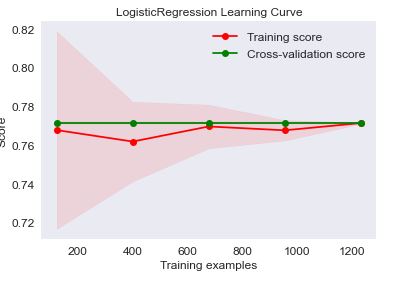
Let’s look at the LogisticRegression Learning Curve
skplt.estimators.plot_learning_curve(LogisticRegression(), X, Y,
cv=7, shuffle=True, scoring=”accuracy”,
n_jobs=-1, figsize=(6,4), title_fontsize=”large”, text_fontsize=”large”,
title=”LogisticRegression Learning Curve”);
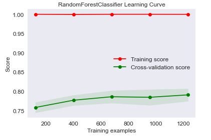
The RandomForestClassifier Learning Curve is
skplt.estimators.plot_learning_curve(RandomForestClassifier(), X, Y,
cv=7, shuffle=True, scoring=”accuracy”,
n_jobs=-1, figsize=(6,4), title_fontsize=”large”, text_fontsize=”large”,
title=”RandomForestClassifier Learning Curve”);
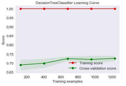
The DecisionTreeClassifier Learning Curve is
from sklearn.tree import DecisionTreeClassifier
skplt.estimators.plot_learning_curve(DecisionTreeClassifier(), X, Y,
cv=7, shuffle=True, scoring=”accuracy”,
n_jobs=-1, figsize=(6,4), title_fontsize=”large”, text_fontsize=”large”,
title=”DecisionTreeClassifier Learning Curve”);
The SVC Learning Curve is
from sklearn.svm import SVC
skplt.estimators.plot_learning_curve(SVC(), X, Y,
cv=7, shuffle=True, scoring=”accuracy”,
n_jobs=-1, figsize=(6,4), title_fontsize=”large”, text_fontsize=”large”,
title=”SVC Learning Curve”);

The ExtraTreesClassifier Learning Curve is
skplt.estimators.plot_learning_curve(ExtraTreesClassifier(), X, Y,
cv=7, shuffle=True, scoring=”accuracy”,
n_jobs=-1, figsize=(6,4), title_fontsize=”large”, text_fontsize=”large”,
title=”ExtraTreesClassifier Learning Curve”);

The XGBClassifier Learning Curve is
from xgboost import XGBClassifier
skplt.estimators.plot_learning_curve(XGBClassifier(), X, Y,
cv=7, shuffle=True, scoring=”accuracy”,
n_jobs=-1, figsize=(6,4), title_fontsize=”large”, text_fontsize=”large”,
title=”XGBClassifier Learning Curve”);

The GradientBoostingClassifier Learning Curve is
skplt.estimators.plot_learning_curve(GradientBoostingClassifier(), X, Y,
cv=7, shuffle=True, scoring=”accuracy”,
n_jobs=-1, figsize=(6,4), title_fontsize=”large”, text_fontsize=”large”,
title=”GradientBoostingClassifier Learning Curve”);

We can see that the GradientBoostingClassifier (GBC) yields the best performance in terms of ML convergence and error bounds of both training and cross-validation scores as functions of 1200+ training examples.
GBC GridSearchCV
Let’s apply GridSearchCV to GBC:
from sklearn.model_selection import GridSearchCV
Create GradientBoostingClassifier
gbc = GradientBoostingClassifier()
parameters = {
“n_estimators”:[5,50,250,500],
“max_depth”:[1,3,5,7,9],
“learning_rate”:[0.01,0.1,1,10,100]
}
Create grid search using 5-fold cross validation
clf = GridSearchCV(gbc,parameters)
Fit grid search
best_model = clf.fit(X_train, Y_train)
y_pred=gbc.fit(X_train, Y_train)
Recall the GBC parameter keys
GradientBoostingClassifier().get_params().keys()
dict_keys(['ccp_alpha', 'criterion', 'init', 'learning_rate', 'loss', 'max_depth', 'max_features', 'max_leaf_nodes', 'min_impurity_decrease', 'min_samples_leaf', 'min_samples_split', 'min_weight_fraction_leaf', 'n_estimators', 'n_iter_no_change', 'random_state', 'subsample', 'tol', 'validation_fraction', 'verbose', 'warm_start'])
Recall the label encoder
Y_test= labelencoder_y.fit_transform(Y_test)
print(labelencoder_y.fit_transform(Y_test))
Let’s look at the classification report
print(classification_report(Y_test, labelencoder_y.fit_transform(gbc.predict(X_test))))
precision    recall  f1-score   support

           0       0.52      0.19      0.28        64
           1       0.80      0.95      0.87       224

    accuracy                           0.78       288
   macro avg       0.66      0.57      0.57       288
weighted avg       0.74      0.78      0.74       288
Recall the label encoder
predict=labelencoder_y.fit_transform(gbc.predict(X_test))
and the libraries of interest
import pandas as pd
import numpy as np
import matplotlib.pyplot as plt
import seaborn as sns
from sklearn.preprocessing import LabelEncoder
from sklearn.feature_selection import SelectKBest, f_classif
from sklearn.model_selection import train_test_split
from sklearn.metrics import accuracy_score, f1_score,classification_report,precision_score,recall_score
from imblearn.over_sampling import SMOTE
from sklearn.linear_model import LogisticRegression
from sklearn.ensemble import RandomForestClassifier
from sklearn.svm import SVC
from xgboost import XGBClassifier
Let’s summarize the classification report
print(‘Accuracy –> ‘,accuracy_score(predict,Y_test))
print(‘F1 Score –> ‘,f1_score(predict,Y_test))
print(‘Classification Report –> \n’,classification_report(predict,Y_test))
Accuracy -->  0.78125
F1 Score -->  0.8711656441717791
Classification Report  -->
               precision    recall  f1-score   support

           0       0.19      0.52      0.28        23
           1       0.95      0.80      0.87       265

    accuracy                           0.78       288
   macro avg       0.57      0.66      0.57       288
weighted avg       0.89      0.78      0.82       288
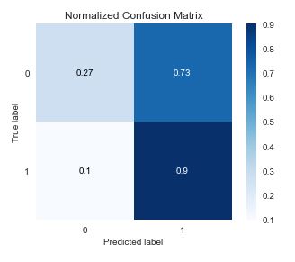
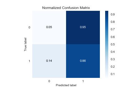
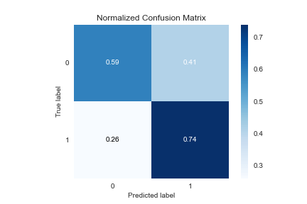
including the normalized confusion matrix
skplt.metrics.plot_confusion_matrix(Y_test, predict, normalize=True)

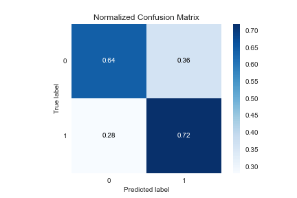
This can be compared against the GBC performance without HPO:
gc=GradientBoostingClassifier(n_estimators=100000,max_depth=5,learning_rate=0.001)
predict=gc.predict(X_test)
predict=labelencoder_y.fit_transform(gc.predict(X_test))
print(‘Accuracy –> ‘,accuracy_score(predict,Y_test))
print(‘F1 Score –> ‘,f1_score(predict,Y_test))
print(‘Classification Report –> \n’,classification_report(predict,Y_test))
print(‘Accuracy –> ‘,accuracy_score(predict,Y_test))
print(‘F1 Score –> ‘,f1_score(predict,Y_test))
print(‘Classification Report –> \n’,classification_report(predict,Y_test))
Accuracy -->  0.7604166666666666
F1 Score -->  0.8541226215644819
Classification Report  -->
               precision    recall  f1-score   support

           0       0.27      0.44      0.33        39
           1       0.90      0.81      0.85       249

    accuracy                           0.76       288
   macro avg       0.58      0.62      0.59       288
weighted avg       0.82      0.76      0.78       288
and the confusion matrix
skplt.metrics.plot_confusion_matrix(Y_test, predict, normalize=True)
ML Performance Plots
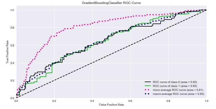
Let’s plot the ROC curve
Y_test_probs = gc.predict_proba(X_test)
skplt.metrics.plot_roc_curve(Y_test, Y_test_probs,
title=”GradientBoostingClassifier ROC Curve”, figsize=(12,6));
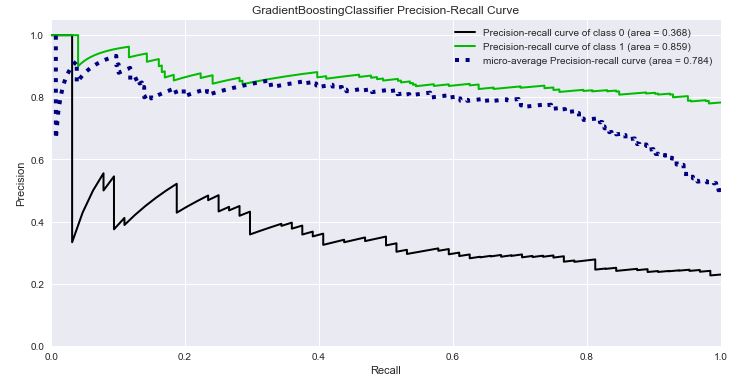
The GradientBoostingClassifier Precision-Recall Curve is
Let’s look at the KMeans clusters
kmeans = KMeans(n_clusters=10, random_state=1)
kmeans.fit(X_train, Y_train)
cluster_labels = kmeans.predict(X_test)
skplt.metrics.plot_silhouette(X_test, cluster_labels,
figsize=(8,6));
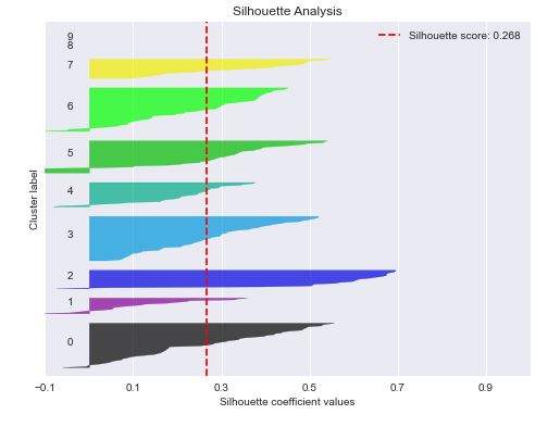
How do I know my silhouette score is good?
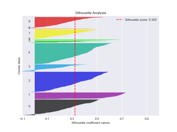
The higher the silhouette score value, the better spread the clusters are.
A silhouette score is great for determining if you have chosen the right number of clusters.
let’s break down the extreme cases of silhouette scores:
1 — This score means that every data point is very compact within the cluster to which it belongs and far away from the other clusters.
0 — Your clusters are overlapping.
-1 — This score means that data belonging to the clusters is incorrect.
As your score tends from 0 to 1, the clusters become more separated and the points within them — closer together. As your score tends from 0 to -1, points may be assigned to the wrong clusters.
Let’s compare calibration curves of various ML algorithms
train_x=X_train
train_y=Y_train
test_x=X_test
lr_probas = LogisticRegression().fit(train_x, train_y).predict_proba(test_x)
rf_probas = RandomForestClassifier().fit(train_x, train_y).predict_proba(test_x)
gb_probas = GradientBoostingClassifier().fit(train_x, train_y).predict_proba(test_x)
et_scores = ExtraTreesClassifier().fit(train_x, train_y).predict_proba(test_x)
probas_list = [lr_probas, rf_probas, gb_probas, et_scores]
clf_names = [‘Logistic Regression’, ‘Random Forest’, ‘Gradient Boosting’, ‘Extra Trees Classifier’]
test_y=Y_test
skplt.metrics.plot_calibration_curve(test_y,
probas_list,
clf_names, n_bins=15,
figsize=(12,6)
);

Let’s look at the GBC KS Statistic plot
rf = GradientBoostingClassifier()
rf.fit(train_x, train_y)
Y_cancer_probas =rf.predict_proba(test_x)
skplt.metrics.plot_ks_statistic(test_y, Y_cancer_probas, figsize=(10,6));

Let’s plot the cumulative gains curve
skplt.metrics.plot_cumulative_gain(test_y, Y_cancer_probas, figsize=(10,6));

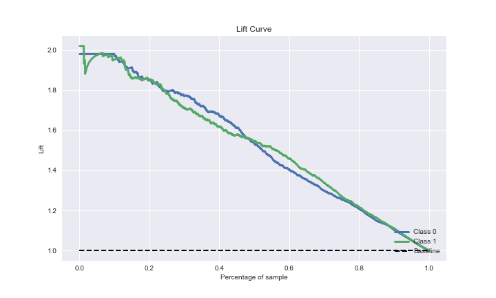
Let’s plot the lift curve
skplt.metrics.plot_lift_curve(test_y, Y_cancer_probas, figsize=(10,6));

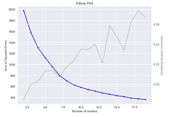
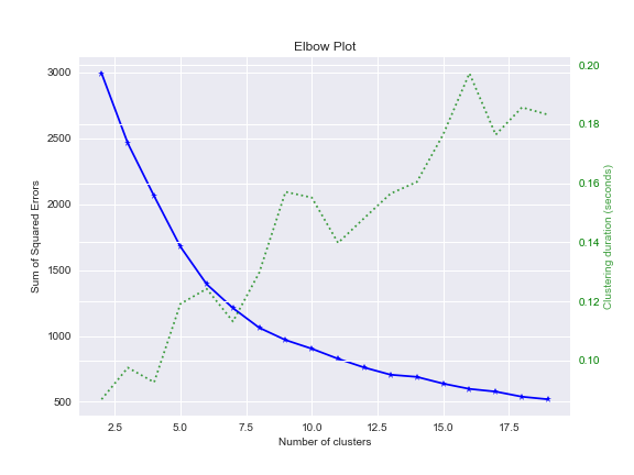
The GBC Kmeans elbow plot is
skplt.cluster.plot_elbow_curve(KMeans(random_state=1),
train_x,
cluster_ranges=range(2, 20),
figsize=(8,6));
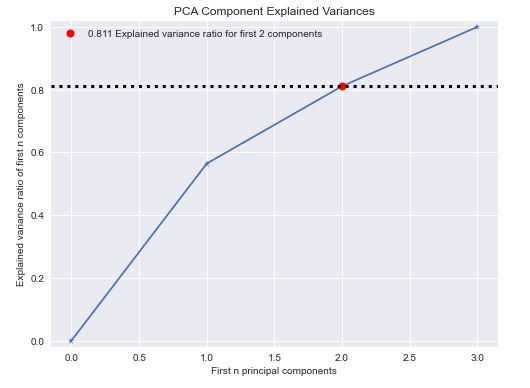
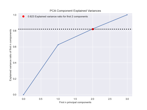
Let’s check the PCA component explained variances
pca = PCA(random_state=1)
pca.fit(train_x)
skplt.decomposition.plot_pca_component_variance(pca, figsize=(8,6));
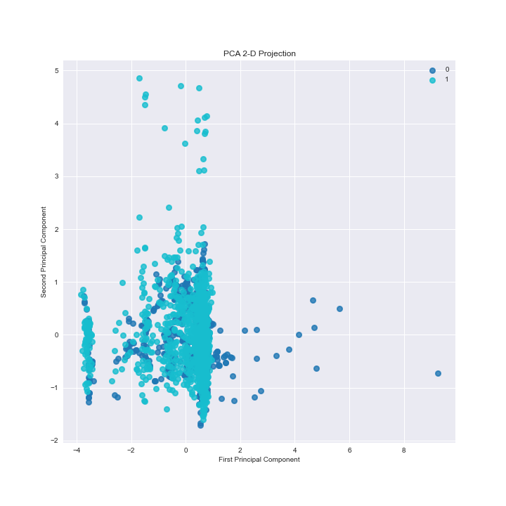
Let’s check the PCA 2-D projection
skplt.decomposition.plot_pca_2d_projection(pca, train_x, train_y,
figsize=(10,10),
cmap=”tab10″);

Data Balancing via Resampling
let’s import additional methods from sklearn.metrics
from sklearn.metrics import precision_score, recall_score, confusion_matrix, classification_report, accuracy_score, f1_score
and check the training and testing data shape
print(f”train data shape:{X_train.shape}”)
print(f”Test data shape:{X_test.shape}”)
train data shape:(1150, 3)
Test data shape:(288, 3)

Base Model
Let’s look at the base GBC model
lreg = GradientBoostingClassifier()
lreg.fit(X_train, Y_train)
GradientBoostingClassifier()
y_pred = lreg.predict(X_test)
y_pred=labelencoder_y.fit_transform(gc.predict(X_test))
y_test=labelencoder_y.fit_transform(y_test)
The classification report is
print (‘Accuracy: ‘, accuracy_score(y_test, y_pred))
print (‘F1 score: ‘, f1_score(y_test, y_pred))
print (‘Recall: ‘, recall_score(y_test, y_pred))
print (‘Precision: ‘, precision_score(y_test, y_pred))
print (‘\n clasification report:\n’, classification_report(y_test,y_pred))
print (‘\n confusion matrix:\n’,confusion_matrix(y_test, y_pred))
Accuracy:  0.7604166666666666
F1 score:  0.8541226215644819
Recall:  0.9017857142857143
Precision:  0.8112449799196787

 clasification report:
               precision    recall  f1-score   support

           0       0.44      0.27      0.33        64
           1       0.81      0.90      0.85       224

    accuracy                           0.76       288
   macro avg       0.62      0.58      0.59       288
weighted avg       0.73      0.76      0.74       288


 confusion matrix:
 [[ 17  47]
 [ 22 202]]
Random OverSampling
Let’s look at random oversampling of the training dataset
from imblearn.over_sampling import RandomOverSampler
over_sample = RandomOverSampler(sampling_strategy = 1)
X_resampled_os, y_resampled_os = over_sample.fit_resample(X_train, Y_train)
len(X_resampled_os)
1770
from collections import Counter
print(sorted(Counter(y_resampled_os).items()))
[(0, 885), (1, 885)]
Let’s make GBC predictions
lreg_os = GradientBoostingClassifier()
lreg_os.fit(X_resampled_os, y_resampled_os)
y_pred_os = lreg_os.predict(X_test)
y_pred_os=labelencoder_y.fit_transform(y_pred_os)
The classification report is
print (‘Accuracy: ‘, accuracy_score(y_test, y_pred_os))
print (‘F1 score: ‘, f1_score(y_test, y_pred_os))
print (‘Recall: ‘, recall_score(y_test, y_pred_os))
print (‘Precision: ‘, precision_score(y_test, y_pred_os))
print (‘\n clasification report:\n’, classification_report(y_test,y_pred_os))
print (‘\n confusion matrix:\n’,confusion_matrix(y_test, y_pred_os))
Accuracy:  0.6805555555555556
F1 score:  0.7766990291262136
Recall:  0.7142857142857143
Precision:  0.851063829787234

 clasification report:
               precision    recall  f1-score   support

           0       0.36      0.56      0.44        64
           1       0.85      0.71      0.78       224

    accuracy                           0.68       288
   macro avg       0.61      0.64      0.61       288
weighted avg       0.74      0.68      0.70       288


 confussion matrix:
 [[ 36  28]
 [ 64 160]]
We can see that RandomOverSampler did not improve prediction results in terms of Accuracy and F1 score.
SMOTE
Let’s invoke SMOTE oversampling
from imblearn.over_sampling import SMOTE
smt = SMOTE(random_state=45, k_neighbors=5)
X_resampled_smt, y_resampled_smt = smt.fit_resample(X_train, y_train)
len(X_resampled_smt)
1770
print(sorted(Counter(y_resampled_smt).items()))
[(0, 885), (1, 885)]
Let’s perform GBC predictions
lreg_smt = GradientBoostingClassifier()
lreg_smt.fit(X_resampled_smt, y_resampled_smt)
y_pred_smt = lreg_smt.predict(X_test)
y_pred_smt=labelencoder_y.fit_transform(y_pred_smt)
The classification report is
print (‘Accuracy: ‘, accuracy_score(y_test, y_pred_smt))
print (‘F1 score: ‘, f1_score(y_test, y_pred_smt))
print (‘Recall: ‘, recall_score(y_test, y_pred_smt))
print (‘Precision: ‘, precision_score(y_test, y_pred_smt))
print (‘\n clasification report:\n’, classification_report(y_test,y_pred_smt))
print (‘\n confusion matrix:\n’,confusion_matrix(y_test, y_pred_smt))
Accuracy:  0.7083333333333334
F1 score:  0.7980769230769232
Recall:  0.7410714285714286
Precision:  0.8645833333333334

 clasification report:
               precision    recall  f1-score   support

           0       0.40      0.59      0.48        64
           1       0.86      0.74      0.80       224

    accuracy                           0.71       288
   macro avg       0.63      0.67      0.64       288
weighted avg       0.76      0.71      0.73       288


 confusion matrix:
 [[ 38  26]
 [ 58 166]]
which looks as follows
predict=y_pred_smt
skplt.metrics.plot_confusion_matrix(Y_test, predict, normalize=True)
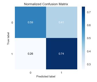
We can see that SMOTE did not improve prediction results in terms of Accuracy and F1 score.
Let’s look at the GBC SMOTE Learning Curve
skplt.estimators.plot_learning_curve(GradientBoostingClassifier(), X_resampled_smt, y_resampled_smt,
cv=7, shuffle=True, scoring=”accuracy”,
n_jobs=-1, figsize=(6,4), title_fontsize=”large”, text_fontsize=”large”,
title=”GradientBoostingClassifier SMOTE Learning Curve”);

Let’s look at the GBC SMOTE ROC Curve
Y_test_probs = gc.predict_proba(X_resampled_smt)
plot=skplt.metrics.plot_roc_curve(y_resampled_smt, Y_test_probs,
title=”GradientBoostingClassifier SMOTE ROC Curve”, figsize=(12,6));
plot.figure.savefig(“gbcsmoterocurve.png”)

The GBC SMOTE Precision-Recall Curve is
plot=skplt.metrics.plot_precision_recall_curve(y_resampled_smt, Y_test_probs,
title=”GradientBoostingClassifier SMOTE Precision-Recall Curve”, figsize=(12,6));
plot.figure.savefig(“gbcsmoteprecisionrecallcurve.png”)

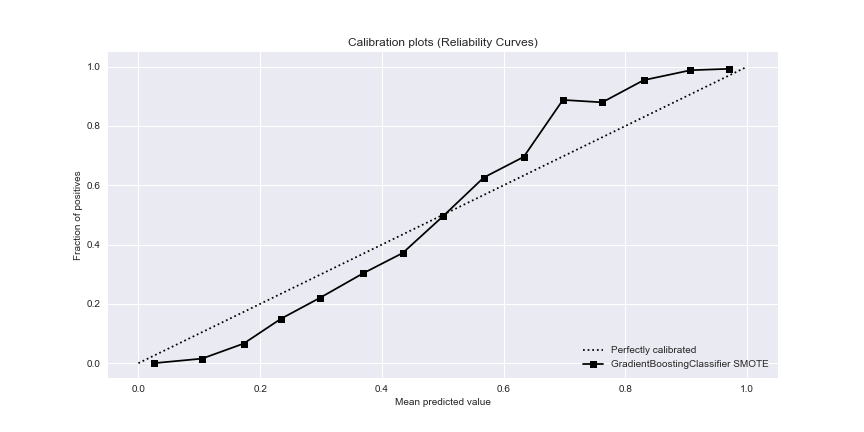
The GBC SMOTE calibration curve is
train_x=X_resampled_smt
train_y=y_resampled_smt
gb_probas = GradientBoostingClassifier().fit(train_x, train_y).predict_proba(X_resampled_smt)
probas_list = [gb_probas]
clf_names = [‘GradientBoostingClassifier SMOTE’]
test_y=y_resampled_smt
plot=skplt.metrics.plot_calibration_curve(test_y,
probas_list,
clf_names, n_bins=15,
figsize=(12,6)
);
plot.figure.savefig(“gbcsmotecalibrationcurve.png”)
The KS Statistic plot is
Y_cancer_probas = rf.predict_proba(X_resampled_smt)
plot=skplt.metrics.plot_ks_statistic(test_y, Y_cancer_probas, figsize=(10,6));
plot.figure.savefig(“gbcsmotekstatistic.png”)

The GBC SMOTE cumulative gain plot is
plot=skplt.metrics.plot_cumulative_gain(test_y, Y_cancer_probas, figsize=(10,6));
plot.figure.savefig(“gbcsmotecumulativegaincurve.png”)

The GBC SMOTE lift plot is
plot=skplt.metrics.plot_lift_curve(test_y, Y_cancer_probas, figsize=(10,6));
plot.figure.savefig(“gbcsmoteliftcurve.png”)

The KMeans silhouette analysis is given by
kmeans = KMeans(n_clusters=10, random_state=1)
kmeans.fit(X_resampled_smt, y_resampled_smt)
cluster_labels = kmeans.predict(X_resampled_smt)
plot=skplt.metrics.plot_silhouette(X_resampled_smt, cluster_labels,
figsize=(8,6));
plot.figure.savefig(“gbcsmotesilhouetteclusters.png”)
The GBC SMOTE elbow plot is
plot=skplt.cluster.plot_elbow_curve(KMeans(random_state=1),
X_resampled_smt,
cluster_ranges=range(2, 20),
figsize=(8,6));
plot.figure.savefig(“gbcsmoteelbowplot.png”)
The GBC SMOTE PCA component explained variances plot is
pca = PCA(random_state=1)
pca.fit(X_resampled_smt)
plot=skplt.decomposition.plot_pca_component_variance(pca, figsize=(8,6));
plot.figure.savefig(“gbcsmotepcavar.png”)
The GBC SMOTE PCA 2-D projection is
plot=skplt.decomposition.plot_pca_2d_projection(pca, X_resampled_smt, y_resampled_smt,
figsize=(10,10),
cmap=”tab10″);
plot.figure.savefig(“gbcsmotepca2dprojection.png”)

ADASYN
Let’s look at the ADASYN data resampling
from imblearn.over_sampling import ADASYN
ada = ADASYN(random_state=45, n_neighbors=5)
X_resampled_ada, y_resampled_ada = ada.fit_resample(X_train, y_train)
len(X_resampled_ada)
1788
The GBC ADASYN learning curve is
plot=skplt.estimators.plot_learning_curve(GradientBoostingClassifier(), X_resampled_ada, y_resampled_ada,
cv=7, shuffle=True, scoring=”accuracy”,
n_jobs=-1, figsize=(6,4), title_fontsize=”large”, text_fontsize=”large”,
title=”GradientBoostingClassifier ADASYN Learning Curve”);
plot.figure.savefig(“gbcadalearningcurve.png”)

The GradientBoostingClassifier ADASYN ROC Curve is
Y_test_probs = gc.predict_proba(X_resampled_ada)
plot=skplt.metrics.plot_roc_curve(y_resampled_ada, Y_test_probs,
title=”GradientBoostingClassifier ADASYN ROC Curve”, figsize=(12,6));
plot.figure.savefig(“gbcadarocurve.png”)

The GradientBoostingClassifier ADASYN Precision-Recall Curve is

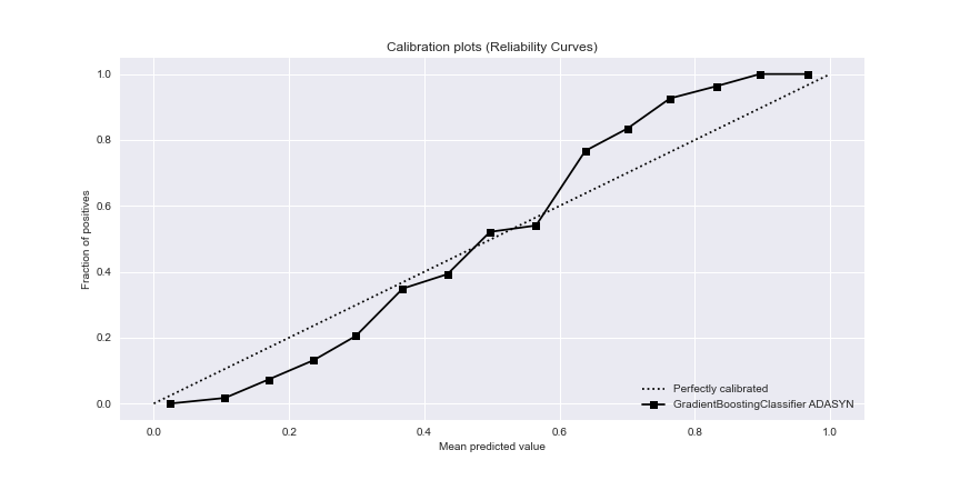
The GradientBoostingClassifier ADASYN calibration curve is
train_x=X_resampled_ada
train_y=y_resampled_ada
gb_probas = GradientBoostingClassifier().fit(train_x, train_y).predict_proba(X_resampled_ada)
probas_list = [gb_probas]
clf_names = [‘GradientBoostingClassifier ADASYN’]
test_y=y_resampled_ada
plot=skplt.metrics.plot_calibration_curve(test_y,
probas_list,
clf_names, n_bins=15,
figsize=(12,6)
);
plot.figure.savefig(“gbcadacalibrationcurve.png”)
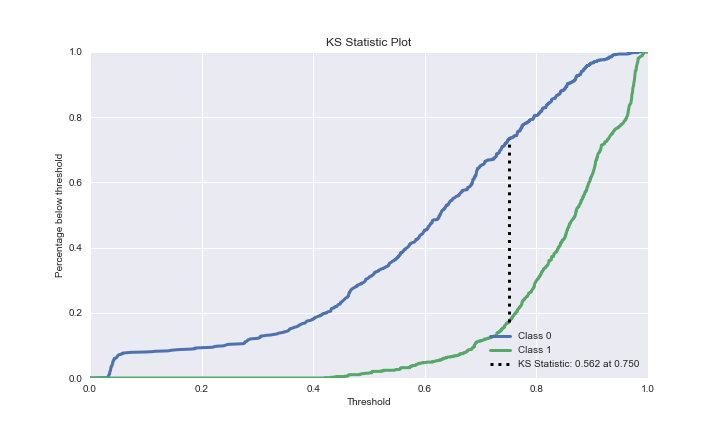
The GBC ADASYN KS Statistic is
Y_cancer_probas = rf.predict_proba(X_resampled_ada)
plot=skplt.metrics.plot_ks_statistic(test_y, Y_cancer_probas, figsize=(10,6));
plot.figure.savefig(“gbcadakstatistic.png”)
The GBC ADASYN cumulative gains curve is
plot=skplt.metrics.plot_cumulative_gain(test_y, Y_cancer_probas, figsize=(10,6));
plot.figure.savefig(“gbcadacumulativegaincurve.png”)

The GBC ADASYN lift curve is
plot=skplt.metrics.plot_lift_curve(test_y, Y_cancer_probas, figsize=(10,6));
plot.figure.savefig(“gbcadaliftcurve.png”)
The KMeans GBC ADASYN silhouette analysis plot is
kmeans = KMeans(n_clusters=10, random_state=1)
kmeans.fit(X_resampled_ada, y_resampled_ada)
cluster_labels = kmeans.predict(X_resampled_ada)
plot=skplt.metrics.plot_silhouette(X_resampled_ada, cluster_labels,
figsize=(8,6));
plot.figure.savefig(“gbcadasilhouette.png”)

The KMeans GBC ADASYN elbow plot is
plot=skplt.cluster.plot_elbow_curve(KMeans(random_state=1),
X_resampled_ada,
cluster_ranges=range(2, 20),
figsize=(8,6));
plot.figure.savefig(“gbcadaelbowplot.png”)

The GBC ADASYN PCA component explained variances plot is
pca = PCA(random_state=1)
pca.fit(X_resampled_ada)
plot=skplt.decomposition.plot_pca_component_variance(pca, figsize=(8,6));
plot.figure.savefig(“gbcadapcavar.png”)

The GBC ADASYN PCA 2-D projection plot is
The GBC ADASYN classification report is
print (‘Accuracy: ‘, accuracy_score(y_test, y_pred_ada))
print (‘F1 score: ‘, f1_score(y_test, y_pred_ada))
print (‘Recall: ‘, recall_score(y_test, y_pred_ada))
print (‘Precision: ‘, precision_score(y_test, y_pred_ada))
print (‘\n clasification report:\n’, classification_report(y_test,y_pred_ada))
print (‘\n confusion matrix:\n’,confusion_matrix(y_test, y_pred_ada))
Accuracy:  0.6597222222222222
F1 score:  0.7537688442211055
Recall:  0.6696428571428571
Precision:  0.8620689655172413

 clasification report:
               precision    recall  f1-score   support

           0       0.35      0.62      0.45        64
           1       0.86      0.67      0.75       224

    accuracy                           0.66       288
   macro avg       0.61      0.65      0.60       288
weighted avg       0.75      0.66      0.69       288


 confusion matrix:
 [[ 40  24]
 [ 74 150]]
ML Classification Reports
Let’s summarize the ML classification reports:
Base Model:
lreg = GradientBoostingClassifier()
lreg.fit(X, Y)
y_pred=labelencoder_y.fit_transform(lreg.predict(X_test))
y_test=labelencoder_y.fit_transform(y_test)
print (‘Accuracy: ‘, accuracy_score(y_test, y_pred))
print (‘F1 score: ‘, f1_score(y_test, y_pred))
print (‘Recall: ‘, recall_score(y_test, y_pred))
print (‘Precision: ‘, precision_score(y_test, y_pred))
print (‘\n classification report:\n’, classification_report(y_test,y_pred))
print (‘\n confusion matrix:\n’,confusion_matrix(y_test, y_pred))
Accuracy:  0.6805555555555556
F1 score:  0.8075313807531381
Recall:  0.8616071428571429
Precision:  0.7598425196850394

 classification report:
               precision    recall  f1-score   support

           0       0.09      0.05      0.06        64
           1       0.76      0.86      0.81       224

    accuracy                           0.68       288
   macro avg       0.42      0.45      0.43       288
weighted avg       0.61      0.68      0.64       288


 confusion matrix:
 [[  3  61]
 [ 31 193]]
predict=y_pred
plot=skplt.metrics.plot_confusion_matrix(Y_test, predict, normalize=True)
plot.figure.savefig(“gbcpredictconfusionmatrix.png”)
RandomOverSampler:
over_sample = RandomOverSampler(sampling_strategy = 1)
X_resampled_os, y_resampled_os = over_sample.fit_resample(X_train, Y_train)
len(X_resampled_os)
1770
lreg_os = GradientBoostingClassifier()
lreg_os.fit(X_resampled_os, y_resampled_os)
y_pred_os = lreg_os.predict(X_test)
y_pred_os=labelencoder_y.fit_transform(y_pred_os)
print (‘Accuracy: ‘, accuracy_score(y_test, y_pred_os))
print (‘F1 score: ‘, f1_score(y_test, y_pred_os))
print (‘Recall: ‘, recall_score(y_test, y_pred_os))
print (‘Precision: ‘, precision_score(y_test, y_pred_os))
print (‘\n classification report:\n’, classification_report(y_test,y_pred_os))
print (‘\n confusion matrix:\n’,confusion_matrix(y_test, y_pred_os))
Accuracy:  0.7048611111111112
F1 score:  0.7921760391198044
Recall:  0.7232142857142857
Precision:  0.8756756756756757

 classification report:
               precision    recall  f1-score   support

           0       0.40      0.64      0.49        64
           1       0.88      0.72      0.79       224

    accuracy                           0.70       288
   macro avg       0.64      0.68      0.64       288
weighted avg       0.77      0.70      0.73       288


 confusion matrix:
 [[ 41  23]
 [ 62 162]]
predict=y_pred_os
plot=skplt.metrics.plot_confusion_matrix(Y_test, predict, normalize=True)
plot.figure.savefig(“gbcpredictosconfusionmatrix.png”)
SMOTE OverSampler:
from imblearn.over_sampling import SMOTE
smt = SMOTE(random_state=45, k_neighbors=5)
X_resampled_smt, y_resampled_smt = smt.fit_resample(X_train, y_train)
len(X_resampled_smt)
1770
lreg_smt = GradientBoostingClassifier()
lreg_smt.fit(X_resampled_smt, y_resampled_smt)
y_pred_smt = lreg_smt.predict(X_test)
y_pred_smt=labelencoder_y.fit_transform(y_pred_smt)
print (‘Accuracy: ‘, accuracy_score(y_test, y_pred_smt))
print (‘F1 score: ‘, f1_score(y_test, y_pred_smt))
print (‘Recall: ‘, recall_score(y_test, y_pred_smt))
print (‘Precision: ‘, precision_score(y_test, y_pred_smt))
print (‘\n classification report:\n’, classification_report(y_test,y_pred_smt))
print (‘\n confusion matrix:\n’,confusion_matrix(y_test, y_pred_smt))
Accuracy:  0.7083333333333334
F1 score:  0.7980769230769232
Recall:  0.7410714285714286
Precision:  0.8645833333333334

 classification report:
               precision    recall  f1-score   support

           0       0.40      0.59      0.48        64
           1       0.86      0.74      0.80       224

    accuracy                           0.71       288
   macro avg       0.63      0.67      0.64       288
weighted avg       0.76      0.71      0.73       288


 confusion matrix:
 [[ 38  26]
 [ 58 166]]
predict=y_pred_smt
plot=skplt.metrics.plot_confusion_matrix(Y_test, predict, normalize=True)
plot.figure.savefig(“gbcpredictsmtconfusionmatrix.png”)
ADASYN OverSampler:
from imblearn.over_sampling import ADASYN
ada = ADASYN(random_state=45, n_neighbors=5)
X_resampled_ada, y_resampled_ada = ada.fit_resample(X_train, y_train)
len(X_resampled_ada)
1788
lreg_ada = GradientBoostingClassifier()
lreg_ada.fit(X_resampled_ada, y_resampled_ada)
y_pred_ada = lreg_ada.predict(X_test)
y_pred_ada=labelencoder_y.fit_transform(y_pred_ada)
print (‘Accuracy: ‘, accuracy_score(y_test, y_pred_ada))
print (‘F1 score: ‘, f1_score(y_test, y_pred_ada))
print (‘Recall: ‘, recall_score(y_test, y_pred_ada))
print (‘Precision: ‘, precision_score(y_test, y_pred_ada))
print (‘\n classification report:\n’, classification_report(y_test,y_pred_ada))
print (‘\n confusion matrix:\n’,confusion_matrix(y_test, y_pred_ada))
Accuracy:  0.6597222222222222
F1 score:  0.7537688442211055
Recall:  0.6696428571428571
Precision:  0.8620689655172413

 classification report:
               precision    recall  f1-score   support

           0       0.35      0.62      0.45        64
           1       0.86      0.67      0.75       224

    accuracy                           0.66       288
   macro avg       0.61      0.65      0.60       288
weighted avg       0.75      0.66      0.69       288


 confusion matrix:
 [[ 40  24]
 [ 74 150]]
predict=y_pred_ada
plot=skplt.metrics.plot_confusion_matrix(Y_test, predict, normalize=True)
plot.figure.savefig(“gbcpredictadaconfusionmatrix.png”)

Summary
Testing ML Models:
| Method/Metrics | Accuracy | F1-Score | Recall | Precision |
| (0) Logistic Regression | 0.77 | 0.87 | 0.96 | 0.79 |
| (1) Linear SVM Classifier | 0.77 | 0.88 | 1.00 | 0.78 |
| (2) RBF Classifier | 0.77 | 0.87 | 0.99 | 0.78 |
| (3) Decision Tree Classifier | 0.75 | 0.84 | 0.85 | 0.83 |
| (4) Random Forest Classifier | 0.77 | 0.86 | 0.91 | 0.82 |
ML Learning Curves:
| Method/Accuracy | Training | X-Validation |
| LogisticRegression | 0.77 | 0.77 |
| RandomForestClassifier | 1.0 | 0.78 |
| DecisionTreeClassifier | 1.0 | 0.72 |
| SVC Classifier | 0.77 | 0.77 |
| ExtraTreesClassifier | 1.0 | 0.77 |
| XGBClassifier | 0.98 | 0.75 |
| GradientBoostingClassifier | 0.86 | 0.78 |
GBC GridSearchCV HPO (Base Model):
Accuracy ~ 0.78
F1-Score ~ 0.87
Recall ~ 0.80
Precision ~0.95
The impact of GBC data resampling alone (without HPO):
| Oversampler/Metrics | Accuracy | F1-Score | Recall | Precision |
| Base Model | 0.68 | 0.71 | 0.86 | 0.76 |
| Random | 0.70 | 0.79 | 0.72 | 0.87 |
| SMOTE | 0.71 | 0.79 | 0.74 | 0.86 |
| ADASYN | 0.66 | 0.75 | 0.67 | 0.86 |
Conclusions
Thus, the key success factors are the GradientBoostingClassifier method combined with GridSearchCV HPO, and data scaling using RobustScaler, followed by SMOTE resampling to balance the “no_fire” and “fire” sets. This yields the maximum precision of 95%, F1-score of 87%, recall of 80%, and X-validation accuracy of 78%. Other ML performance KPI’s are as follows: ROC = 0.97, precision-recall = 0.96, KS Statistic – 0.59 at 0.75, max lift = 2.0, silhouette score = 0.325, number of clusters = 7, explained variance ratio for first 2 components = 0.823. The PCA 2-D projection shows only partial separation of clusters CLASS =0, 1.
References
[1] Younes OuladSayad HajarMousannif HassanAl Moatassime, Predictive modeling of wildfires: A new dataset and machine learning approach, Volume 104, March 2019, Pages 130-146. https://doi.org/10.1016/j.firesaf.2019.01.006
[2] Piyush Jain piyush.jain@canada.ca, Sean C.P. Coogan, Sriram Ganapathi Subramanian, Mark Crowley, Steve Taylor, and Mike D. Flannigan, A review of machine learning applications in wildfire science and management, Environmental Reviews 28 July 2020 https://doi.org/10.1139/er-2020-0019.
[3] Forest Fire prediction using Machine Learning
[4] Towards Optimized ML Wildfire Prediction
[7] Ruth Coughlan,Francesca Di Giuseppe,Claudia Vitolo,Christopher Barnard,Philippe Lopez,Matthias Drusch, Using machine learning to predict fire-ignition occurrences from lightning forecasts, RMetS, 1 January 2021 https://doi.org/10.1002/met.1973


Leave a comment