AI-Guided Drug Recommendation

The use of data analytics (DA) and artificial intelligence (AI) have been increasing in the pharmaceutical industry, including drug R&D, drug repurposing, improving pharmaceutical productivity, and clinical trials, among others. DA uses algorithms that can recognize patterns within a set of data to be further classified. Examples include drug recommendation, discovery and validation using knowledge graphs and Natural Language Processing (NLP) algorithms.

Leading biopharmaceutical companies’ belief in AI is due to growing awareness related to AI in the pharmaceutical sector and rising investment in drug development.

Contents:

1. E2E Workflow
2. Import Libraries
3. Input Data
4. Raw Data Cleaning
5. Exploratory Data Analysis (EDA)
6. Review Sentiments
7. WordCloud Images
8. Review Sentiment Editing
9. Text Data Pre-Processing
10. Sentiment Correlations
11. Review Data Editing
12. Feature Engineering
13. NER Analysis
14. Topic Modelling
15. Train LDA
16. Topic Correlations
17. NLP Modelling
18. BoW Vectorizer
19. TF-IDF Vectorizer
20. Word2Vec Vectorizer
21. NLP Modelling
22. Conclusion
23. Appendix:
24. Multi-Cloud NLP Drug Recommendation

Following the earlier DA-based study (cf. research paper and the source code), the objective of this project is to to build an AI-guided drug review system that recommends the most effective drug for a certain condition based on available reviews of various drugs used to treat this condition.

E2E Workflow

• Setup Jupyter notebook within the Anaconda IDE
• Import/install relevant Python libraries
• Download the Kaggle UCI ML Drug Review dataset
• Overview of the train/test dataset
• Reset the index after data concatenation
• Exploratory Data Analysis (EDA) using SNS plots
• Plot the WordCount images for positive/negative reviews
• Loading stop words from NLTK
• Text data NLP Pre-Processing (removing digits, extra spaces, lower case, etc.)
• nltk.sentiment.vader sentiment analysis using SentimentIntensityAnalyzer
• Adding the sentiment scores for reviews, preprocessed reviews as new features
• Feature Engineering – check the Pearson correlation matrix of various features
• Adding the word count, stopword count,char length, unique words count, mean word length, and puncation count
• Named entity recognition (NER) using spacy
• LDA topic modelling – prepare cleaned reviews
• Splitting the data into train, test and cross-validation (CV) datasets
• Encoding categorical, text and numerical features by applying LabelEncoder
• Vectorizing the cleaned reviews using BoW, TF-IDF (1 gram)
• Word2Vec Vectorization for reviews using pretrained glove model
• Compute the LDA confusion, precision, and recall matrices for the test data

Import Libraries

Let’s set the working directory YOURPATH

import os
os. getcwd()

os.chdir(‘YOURPATH’)

and import/install relevant Python libraries

import pandas as pd
import numpy as np
import matplotlib.pyplot as plt
import seaborn as sns
import warnings
warnings.filterwarnings(‘ignore’)
from wordcloud import WordCloud
from wordcloud import STOPWORDS

import nltk
import regex as re
from nltk.corpus import stopwords
from nltk.stem.snowball import SnowballStemmer

import re
from tqdm import tqdm
from nltk.corpus import stopwords

from nltk.sentiment.vader import SentimentIntensityAnalyzer

import string

import spacy

from tqdm import tqdm

import gensim

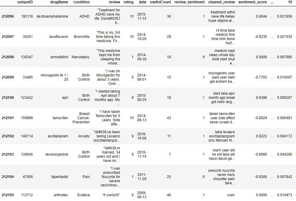
Input Data

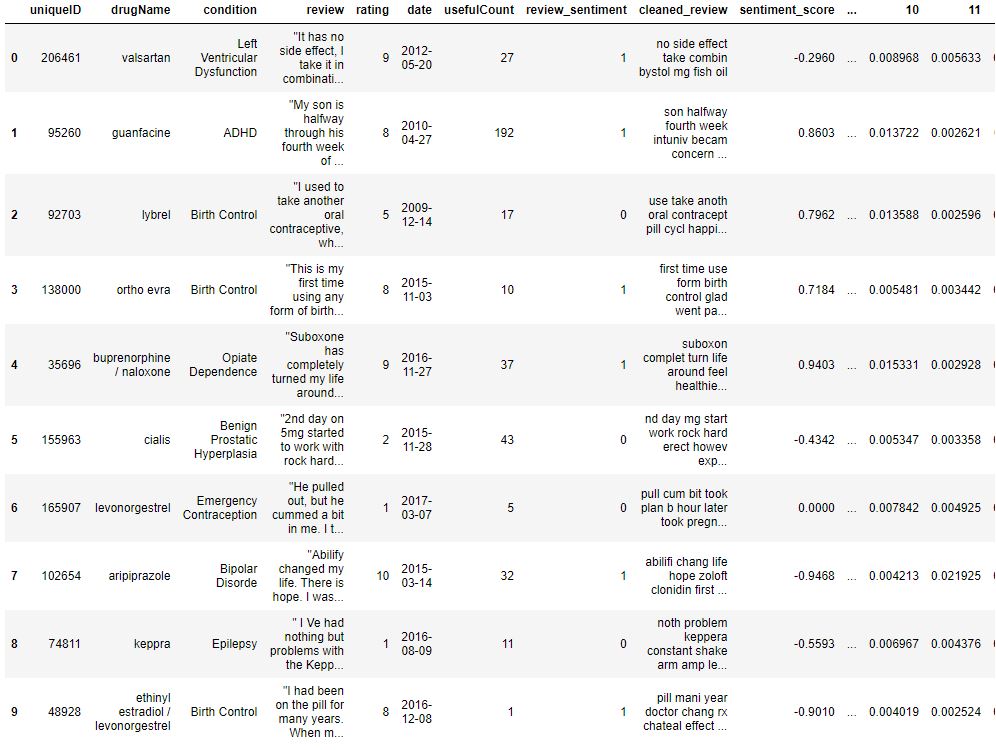
Let’s read the Kaggle train and test data as csv files

data_train = pd.read_csv(‘drugsComTrain_raw.csv’)
data_test = pd.read_csv(‘drugsComTest_raw.csv’)

and check the dataset structure

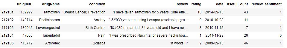
print(‘Size of Train dataset is:’,data_train.shape)
print(‘Size of Test dataset is:’,data_test.shape)

Size of Train dataset is: (161297, 7)
Size of Test dataset is: (53766, 7)

print(‘Columns of the dataset are:\n’,data_train.columns)

Columns of the dataset are:
 Index(['uniqueID', 'drugName', 'condition', 'review', 'rating', 'date',
       'usefulCount'],
      dtype='object')

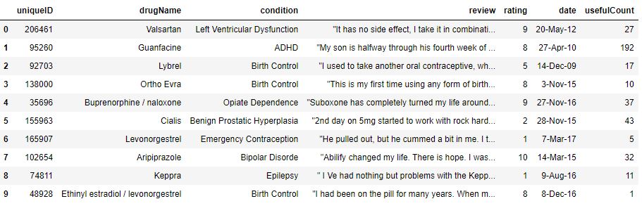
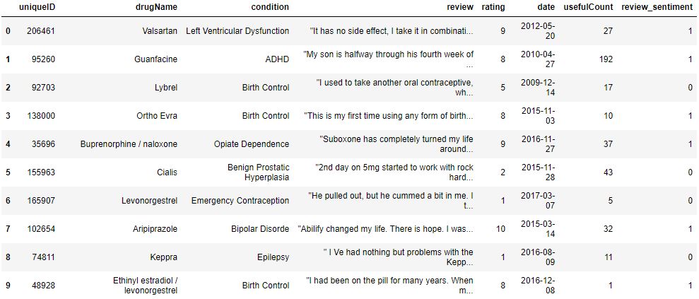
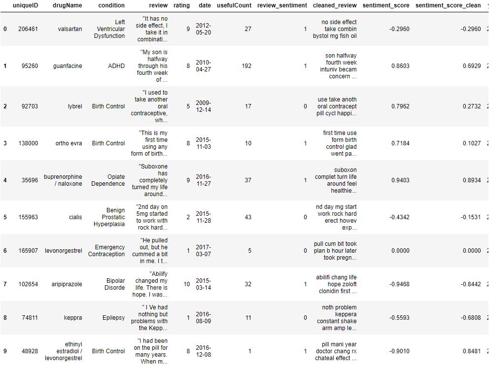
print(‘Overview of Train dataset:\n’)
data_train.head(10)

Overview of Train dataset:

Similarly, let’s print the test Kaggle dataset

print(‘Overview of Test dataset:\n’)
data_test.head(10)

Overview of Test dataset:

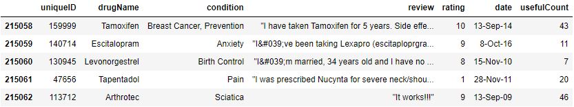
Let’s concatenate the two datasets

data = pd.concat([data_train,data_test])
print(‘The size of the combined data is:’,data.shape)

The size of the combined data is: (215063, 7)

while resetting the index after concatenation

data.reset_index(inplace=True,drop=True)
data.tail()

Let’s verify data types
data.dtypes

uniqueID        int64
drugName       object
condition      object
review         object
rating          int64
date           object
usefulCount     int64
dtype: object

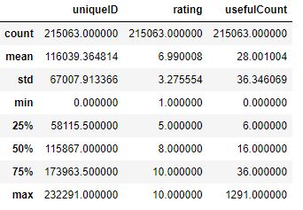
The descriptive statistics of numerical features is given by

data.describe()

and the data info is

data.info()

<class 'pandas.core.frame.DataFrame'>
RangeIndex: 215063 entries, 0 to 215062
Data columns (total 7 columns):
 #   Column       Non-Null Count   Dtype 
---  ------       --------------   ----- 
 0   uniqueID     215063 non-null  int64 
 1   drugName     215063 non-null  object
 2   condition    213869 non-null  object
 3   review       215063 non-null  object
 4   rating       215063 non-null  int64 
 5   date         215063 non-null  object
 6   usefulCount  215063 non-null  int64 
dtypes: int64(3), object(4)
memory usage: 11.5+ MB

Raw Data Cleaning

Let’s check the above data for null values
data.isnull().any()

uniqueID       False
drugName       False
condition       True
review         False
rating         False
date           False
usefulCount    False
dtype: bool

and the percentage of null values is

null_size = data.isnull().sum()[‘condition’]
print(‘Total null values are:’,null_size)
data_size = data.shape[0]
print(‘Percentage of null values are:’,(null_size/data_size)*100)

Total null values are: 1194
Percentage of null values are: 0.5551861547546533

Let’ drop the entire rows with null values

data = data.dropna(axis=0)
print(‘Size of the dataset after dropping null values:’,data.shape)

Size of the dataset after dropping null values: (213869, 7)

and check for number of unique conditions

print(‘Number of unique conditions are:’,data[‘condition’].unique().shape[0])

Number of unique conditions are: 916

Exploratory Data Analysis (EDA)

Referring to the previous DA analysis, let’s apply EDA to our data after dropping null values.

Let’s plot the top 10 conditions

conditions = dict(data[‘condition’].value_counts())
top_conditions = list(conditions.keys())[0:10]
values = list(conditions.values())[0:10]
plt.figure(figsize=(16,8))
sns.set_style(style=’darkgrid’)
b=sns.barplot(x=top_conditions,y=values,palette=’spring’)
plt.title(‘Top 10 Conditions’)
plt.xlabel(‘Conditions’)
plt.ylabel(‘Count’)
plt.xticks(fontsize=11)
plt.yticks(fontsize=11)
b.set_xlabel(“Conditions”,fontsize=20)
b.set_ylabel(“Count”, fontsize=20)
b.tick_params(labelsize=12)
b.axes.set_title(“Top 10 Conditions”,fontsize=20)
plt.show()
plt.savefig(‘drugbartop10conditions.png’)

It is clear that Birth Control is the most frequently occurring condition in our dataset, followed by Depression, Pain, Anxiety, etc.

Let’s count the number of drugs provided or prescribed as a treatment for top 10 conditions

val=[]
for c in list(conditions.keys()):
val.append(data[data[‘condition’]==c][‘drugName’].nunique())

drug_cond = dict(zip(list(conditions.keys()),val))

Let’s plot the number of drugs provided or prescribed as a treatment for top 10 conditions
top_conditions = list(drug_cond.keys())[0:10]
values = list(drug_cond.values())[0:10]
plt.figure(figsize=(16,8))
sns.set_style(style=’darkgrid’)
b=sns.barplot(x=top_conditions,y=values,palette=’spring’)
plt.title(‘Number of Drugs for each Top 10 Conditions’)
plt.xlabel(‘Conditions’)
plt.ylabel(‘Count of Drugs’)

b.set_xlabel(“Count of Patients used”,fontsize=20)
b.set_ylabel(“Drug Names”, fontsize=20)
b.tick_params(labelsize=12)
b.axes.set_title(“Number of Drugs for each Top 10 Conditions”,fontsize=20)

plt.show()
plt.savefig(‘drugbarnumberofdrugs.png’)

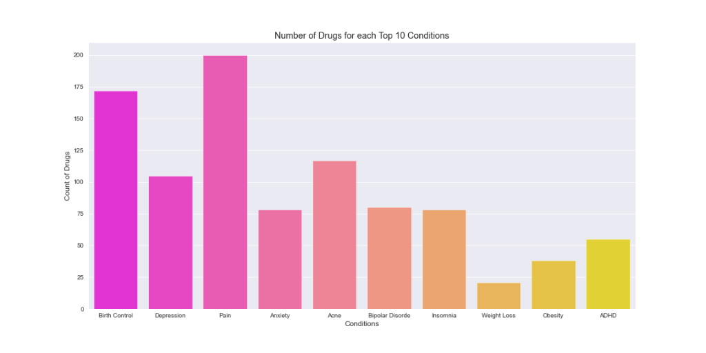
This plot shows that multiple drugs are normally used as a treatment for top 10 conditions. It seems that there will likely be no “silver bullet” medication for Pain and Birth Control conditions.

Let’s see what is the most frequently used Birth Control drug by plotting top 10 drugs used as a treatment for this particular condition

drugs_birth = dict(data[data[‘condition’]==’Birth Control’][‘drugName’].value_counts())

top_drugs = list(drugs_birth.keys())[0:10]
values = list(drugs_birth.values())[0:10]
plt.figure(figsize=(16,8))
sns.set_style(style=’darkgrid’)
b=sns.barplot(x=values,y=top_drugs,palette=’spring’)
plt.title(‘Top 10 Drugs used for Birth Control’)
plt.ylabel(‘Drug Names’)
plt.xlabel(‘Count of Patients used’)

b.set_xlabel(“Count of Patients used”,fontsize=20)
b.set_ylabel(“Drug Names”, fontsize=20)
b.tick_params(labelsize=12)
b.axes.set_title(“Top 10 Drugs used for Birth Control”,fontsize=20)

plt.show()
plt.savefig(‘drugbarnumbermostuseddrugs.png’)

It is clear that Etonogestrel is the most frequently used Birth Control drug, followed by Ethinyl estradiol, Levonorgestrel and Nexplanon.

Similarly, we can plot top 10 drugs used as a treatment for Pain

drugs_pain = dict(data[data[‘condition’]==’Pain’][‘drugName’].value_counts())

top_drugs = list(drugs_pain.keys())[0:10]
values = list(drugs_pain.values())[0:10]
plt.figure(figsize=(16,8))
sns.set_style(style=’darkgrid’)
b=sns.barplot(x=values,y=top_drugs,palette=’spring’)
plt.title(‘Top 10 Drugs used for Pain’)
plt.ylabel(‘Drug Names’)
plt.xlabel(‘Count of Patients used’)

b.set_xlabel(“Count of Patients used”,fontsize=20)
b.set_ylabel(“Drug Names”, fontsize=20)
b.tick_params(labelsize=12)
b.axes.set_title(“Top 10 Drugs used for Pain”,fontsize=20)

plt.show()
plt.savefig(‘drugbarnumbermostusedpain.png’)

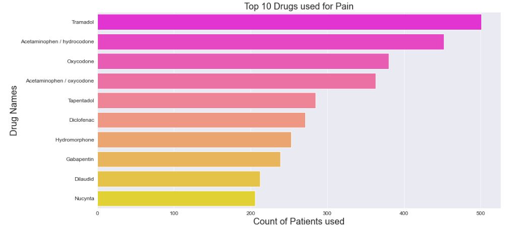
We can see that Tramadol is the most frequently used Pain drug.

Let’s plot the top 10 drugs rated as 10
drugs_rating = dict(data[data[‘rating’]==10][‘drugName’].value_counts())

top_drugs = list(drugs_rating.keys())[0:10]
values = list(drugs_rating.values())[0:10]
plt.figure(figsize=(16,8))
sns.set_style(style=’darkgrid’)
b=sns.barplot(x=values,y=top_drugs,palette=’spring’)
plt.title(‘Top 10 Drugs rated as 10’)
plt.ylabel(‘Drug Names’)
plt.xlabel(‘Count of Ratings’)

b.set_xlabel(“Count of Ratings”,fontsize=20)
b.set_ylabel(“Drug Names”, fontsize=20)
b.tick_params(labelsize=12)
b.axes.set_title(“Top 10 Drugs rated as 10”,fontsize=20)

plt.show()
plt.savefig(‘drugbartop10rate10.png’)

It appears that Birth Control drugs are top rated, so Etonogestrel and Levonorgestrel should be the top recommended drugs as they are (a) most frequently used and (b) rated as 10 by patients.

Likewise, let’s plot the top 10 drugs rated as 1

drugs_rating = dict(data[data[‘rating’]==1][‘drugName’].value_counts())

top_drugs = list(drugs_rating.keys())[0:10]
values = list(drugs_rating.values())[0:10]
plt.figure(figsize=(16,8))
sns.set_style(style=’darkgrid’)
b=sns.barplot(x=values,y=top_drugs,palette=’spring’)
plt.title(‘Top 10 Drugs rated as 1’)
plt.ylabel(‘Drug Names’)
plt.xlabel(‘Count of Ratings’)

b.set_xlabel(“Count of Ratings”,fontsize=20)
b.set_ylabel(“Drug Names”, fontsize=20)
b.tick_params(labelsize=12)
b.axes.set_title(“Top 10 Drugs rated as 1”,fontsize=20)

plt.show()
plt.savefig(‘drugbartop10rate1.png’)

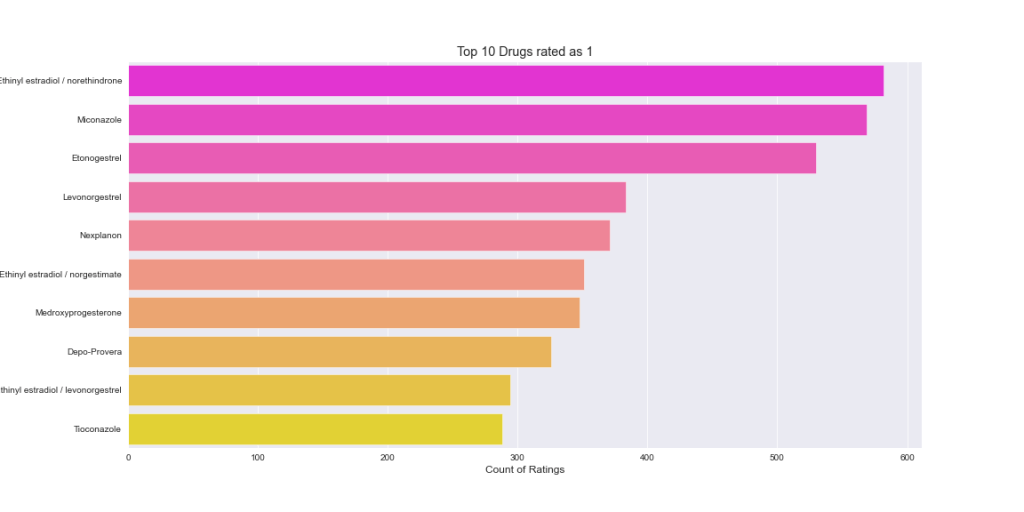
One can see that Levonorgestrel and Etonogestrel are among top 10 most frequently used drugs that have both ratings ‘10’ and ‘1’. The lowest rating may imply that these two drugs had side effects and/or not effective for certain patients.

Let’s plot the density distributions of ratings 1-10
f,ax = plt.subplots(1,2,figsize=(16,8))
ax1= sns.histplot(data[‘rating’],ax=ax[0])
ax1.set_title(‘Count of Ratings’)
ax2= sns.distplot(data[‘rating’],ax=ax[1],color=”r”)
ax2.set_title(‘Distribution of Ratings density’)
ax2.axes.set_title(“Distribution of Ratings Density”,fontsize=20)
ax2.set_xlabel(“Rating”,fontsize=20)
ax2.set_ylabel(“Count”, fontsize=20)
ax2.tick_params(labelsize=12)

ax1.set_xlabel(“Rating”,fontsize=20)
ax1.set_ylabel(“Count”, fontsize=20)
ax1.tick_params(labelsize=12)
ax1.axes.set_title(“Count of Ratings”,fontsize=20)

plt.show()
plt.savefig(‘drugdistplotratingsdens.png’)

We can see that rating 10 has the maximum density or frequency count.

Let’s look at the percentage distribution of ratings using pie chart

ratings_count = dict(data[‘rating’].value_counts())
count = list(ratings_count.values())
labels = list(ratings_count.keys())
plt.figure(figsize=(18,9))
plt.pie(count,labels=labels, autopct=’%1.1f%%’,textprops={‘fontsize’: 14})
plt.title(‘Pie Chart Representation of Ratings’,fontsize=20)
plt.legend(title=’Ratings’,fontsize=12)
plt.show()
plt.savefig(‘drugspiechartratings.png’)

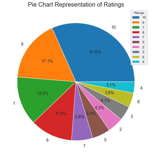
We can see that 31.6% and 13.5% drugs have ratings 10 and 1, respectively.

Let’s change the date format using to_datetime

data[‘date’]= pd.to_datetime(data[‘date’])

and count ratings per year

year_ratings = dict(data[‘date’].dt.year.value_counts())
years = list(year_ratings.keys())
values = list(year_ratings.values())
plt.figure(figsize=(18,9))
b=sns.barplot(x=years,y=values,palette=’spring’)
plt.xlabel(‘Years’)
plt.ylabel(‘Count of Ratings’)
plt.title(‘Count of Ratings in each Year’)
b.set_xlabel(“Year”,fontsize=20)
b.set_ylabel(“Count of Ratings”, fontsize=20)
b.tick_params(labelsize=12)
b.axes.set_title(“Count of Ratings in each Year”,fontsize=20)
plt.show()
plt.savefig(‘drugsbarratingsyear.png’)

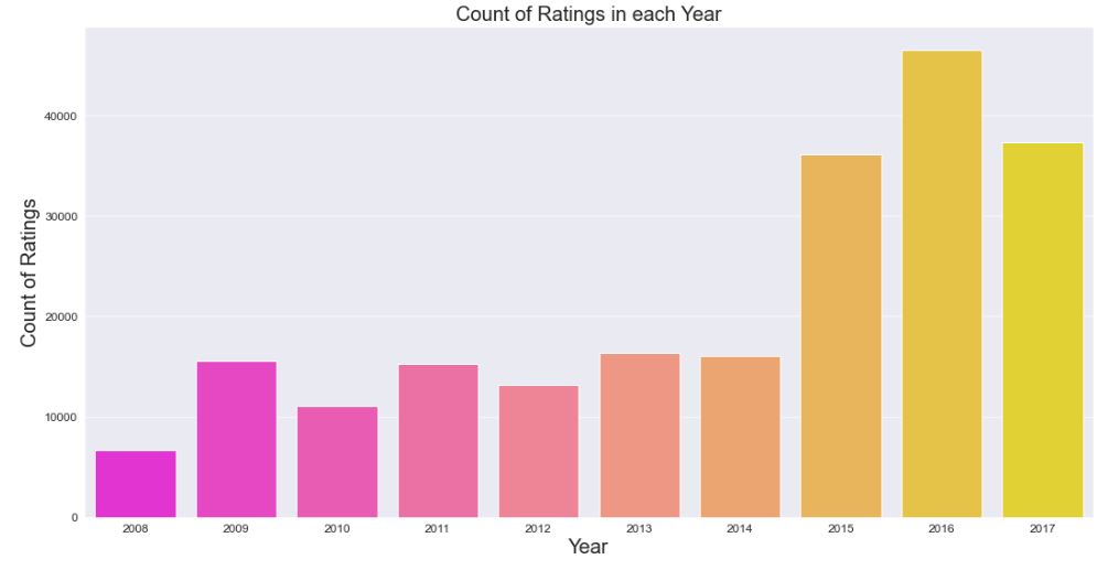
Notably drug ratings achieved their over-4000 peak in 2016.

Let’s check the distribution of usefulCount

plt.figure(figsize=(16,8))
plt.xlim(0, 200)
ax1 =sns.distplot(data[‘usefulCount’],color=’r’,bins=256)
ax1.set_xlabel(“usefulCount”,fontsize=20)
ax1.set_ylabel(“Density”, fontsize=20)
ax1.tick_params(labelsize=12)
plt.title(‘Distribution of usefulCount’,fontsize=20)
plt.show()
plt.savefig(‘drugdistusefulcount.png’)

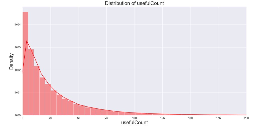
It is clear that there that the feature usefulCount has the limit of 200.

Review Sentiments

Let’s create the target feature review_sediment using ratings

data[‘review_sentiment’] = data[‘rating’].apply(lambda x: 1 if x > 5 else 0)

Here 1 and 0 represent positive and negative reviews, respectively.

data.head(10)

Let’s plot the pie chart for review sentiments

plt.figure(figsize=(14,7))
plt.pie(data[‘review_sentiment’].value_counts(),labels=[‘Positive’,’Negative’],autopct=’%1.1f%%’,textprops={‘fontsize’: 16})
plt.title(‘Pie Chart Representation of Review Sentiment’,fontsize=20)

plt.show()
plt.savefig(‘drugspiechartratings.png’)

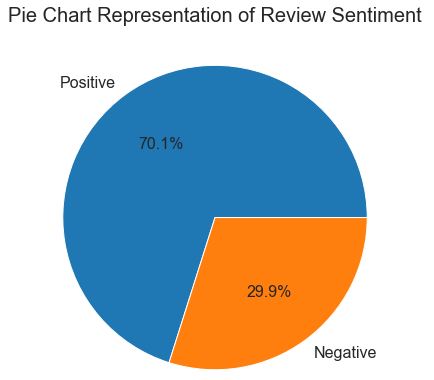
According to this chart, 70.1% of patients are likely to give positive reviews. Hence, this is an imbalanced dataset.

WordCloud Images

Let’s turn our attention to WordCloud – a technique for visualising frequent words in a text where the size of the words represents their frequency.

Let’s look at WordCloud for positive reviews

positive_reviews = ” “.join([review for review in data[‘review’][data[‘review_sentiment’] == 1]])

stop_words = set(STOPWORDS)

wordcloud = WordCloud(width = 1200, height = 800,background_color =’white’,stopwords = stop_words,min_font_size = 10).generate(positive_reviews)

while plotting the WordCloud image

plt.figure(figsize = (12, 8), facecolor = None)
plt.imshow(wordcloud)
plt.title(‘WordCloud for Positive Reviews’)
plt.axis(“off”)
plt.tight_layout(pad = 0)
plt.show()
plt.savefig(‘drugswordcloudpos.png’)

Similarly, we can apply WordCloud to negative reviews

negative_reviews = ” “.join([review for review in data[‘review’][data[‘review_sentiment’] == 0]])

wordcloud = WordCloud(width = 1200, height = 800,background_color =’white’,stopwords = stop_words,min_font_size = 10).generate(negative_reviews)

and plot the resulting image

plt.figure(figsize = (12, 8), facecolor = None)
plt.imshow(wordcloud)
plt.title(‘WordCloud for Negative Reviews’)
plt.axis(“off”)
plt.tight_layout(pad = 0)
plt.show()
plt.savefig(‘drugswordcloudneg.png’)

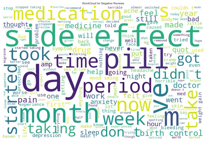
We can see that both positive and negative reviews contain most frequent words “side effect”, “day”, and “period”.

Review Sentiment Editing

Let’s remove some unwanted conditions in the review sentiment data

del_index = []
conds =[]
for c in data[‘condition’]:
if (‘helpful’ in c) or (‘Listed’ in c):
f= list(data[data[‘condition’]==c].index)
del_index.extend(f)
conds.append(c)

print(‘Size of the data before removing the conditions:’,data.shape)

Size of the data before removing the conditions: (213869, 8)

print(‘The removable conditions count is:’,len(conds))

The removable conditions count is: 1763

data.drop(del_index,inplace=True)
print(‘Size of the data after dropping the condtions:’,data.shape)

Size of the data after dropping the condtions: (212106, 8)

data.reset_index(inplace=True,drop=True)
data.tail()

Text Data Pre-Processing

We need to invoke several functions to clean and preprocess the review text data by removing html tags, punctuations, special characters, stopwords, tabs, new lines, spaces and also stemming of words:

def decontracted(phrase):
# specific
phrase = re.sub(r”won’t”, “will not”, phrase)
phrase = re.sub(r”can\’t”, “can not”, phrase)

# general
phrase = re.sub(r"n\'t", " not", phrase)
phrase = re.sub(r"\'re", " are", phrase)
phrase = re.sub(r"\'s", " is", phrase)
phrase = re.sub(r"\'d", " would", phrase)
phrase = re.sub(r"\'ll", " will", phrase)
phrase = re.sub(r"\'t", " not", phrase)
phrase = re.sub(r"\'ve", " have", phrase)
phrase = re.sub(r"\'m", " am", phrase)
return phrase

def preprocess_text(text_data):

text_data = decontracted(text_data)

text_data = text_data.replace('\n',' ')
text_data = text_data.replace('\r',' ')
text_data = text_data.replace('\t',' ')
text_data = text_data.replace('-',' ')
text_data = text_data.replace("/",' ')
text_data = text_data.replace(">",' ')
text_data = text_data.replace('"',' ')
text_data = text_data.replace('?',' ')
return text_data

Let’s load stop words from the nltk library

stop_words = set(stopwords.words(‘english’))
stemmer = SnowballStemmer(‘english’)

Let’s remove ‘no’ from the stop words list due to the importance of ‘side effects’ and ‘no side effects’ in reviews
stop_words.remove(‘no’)

Let’s define the functional block that process the text data by removing digits, extra spaces, stop words, while converting words to lower case and stemming words

def nlp_preprocessing(review):

if type(review) is not int:
string = “”
review = preprocess_text(review)
review = re.sub(‘[^a-zA-Z]’, ‘ ‘, review)

    review = re.sub('\s+',' ', review)

    review = review.lower()

    for word in review.split():

        if not word in stop_words:
            word = stemmer.stem(word)
            string += word + " "

    return string 

Let’s apply the NLP processing

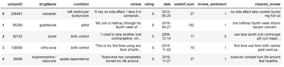
data[‘cleaned_review’] = data[‘review’].apply(nlp_preprocessing)

and convert the content of drugName and condition to lower case

data[‘drugName’] = data[‘drugName’].apply(lambda x:x.lower())

data[‘condition’] = data[‘condition’].apply(lambda x:x.lower())

data.head()

data.shape

(212106, 9)

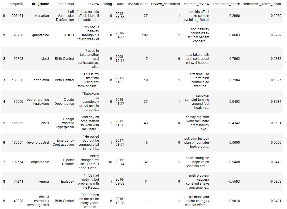
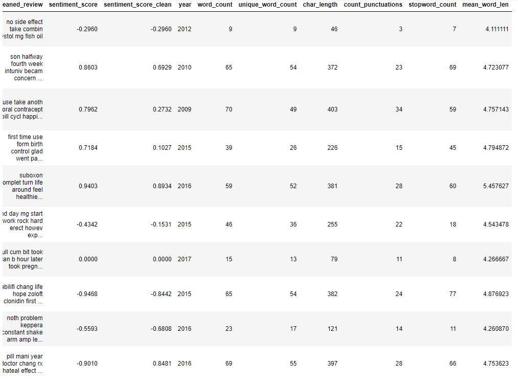
Let’s add the sentiment scores for reviews and preprocessed reviews as new features using SentimentIntensityAnalyzer

sid = SentimentIntensityAnalyzer()
data[‘sentiment_score’] = [sid.polarity_scores(v)[‘compound’] for v in data[‘review’]]
data[‘sentiment_score_clean’] = [sid.polarity_scores(v)[‘compound’] for v in data[‘cleaned_review’]]

data.head()

These text features and sentiment scores are the basic feature extractions for the text data classification problem.

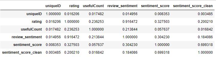
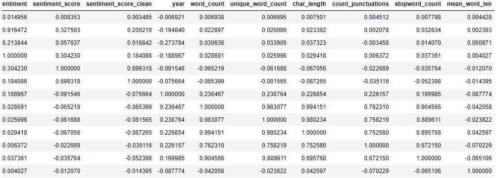
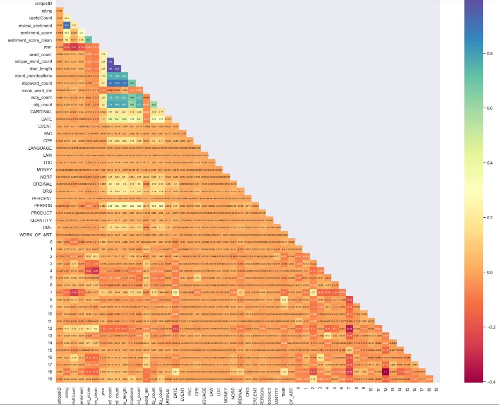
Sentiment Correlations

Let’s check the crrelation of features present in the sentiment data

data.corr()

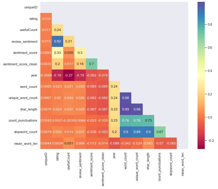
Let’s plot the Pearson’s correlation heatmap lower triangle with Seaborn

corr_data = data.corr(method=’pearson’)

mask_ut=np.triu(np.ones(corr_data.shape)).astype(np.bool)

f, ax = plt.subplots(figsize=(11, 9))
sns.set(font_scale=1)
cmap = sns.diverging_palette(220, 10, as_cmap=True)

sns.heatmap(corr_data, mask=mask_ut, cmap=cmap,annot=True, annot_kws={“size”:16})
hmap.figure.savefig(“Correlation_Heatmap_Lower_Triangle_with_Seaborn.png”,
format=’png’,
dpi=150)

Let’s save the data for future reference

data.to_csv(‘new_data_processed.csv’,index=False)

Review Data Editing

Let’s check the content of data

data.head(10)

checking for any nan values in cleaned_review feature

data[‘cleaned_review’].isna().sum()

0

and droping all rows containing nan values

print(‘The data size before:’,data.shape)
data = data.dropna(axis=0)
data.reset_index(inplace=True,drop=True)
print(‘The data size after dropping:’,data.shape)

The data size before: (212106, 11)
The data size after dropping: (212106, 11)

We can see that there are no nan values in our processed dataset

Let’s add the year as feature and check the data structure

data[‘date’] = pd.to_datetime(data[‘date’])
data[‘year’] = data[‘date’].dt.year
data.head(10)

Let’s add the word count, stopword count, char length, unique words count, mean word length, and puncation count

stop_words = set(stopwords.words(‘english’))

data[‘word_count’]=data[“cleaned_review”].apply(lambda x: len(str(x).split()))

data[‘unique_word_count’]=data[“cleaned_review”].apply(lambda x: len(set(str(x).split())))

data[‘char_length’]=data[“cleaned_review”].apply(lambda x: len(str(x)))

data[“count_punctuations”] = data[“review”].apply(lambda x: len([c for c in str(x) if c in string.punctuation]))

data[“stopword_count”] = data[“review”].apply(lambda x: len([w for w in str(x).lower().split() if w in stop_words]))

data[“mean_word_len”] = data[“cleaned_review”].apply(lambda x: np.mean([len(w) for w in str(x).split()]))

Let’s check the updated content

data.head(10)

Feature Engineering

Let’s compute data correlations

Let’s compute the correlation heatmap lower triangle with seaborn

corr1_data = data.corr(method=’pearson’)
mask_ut=np.triu(np.ones(corr1_data.shape)).astype(np.bool)

f, ax = plt.subplots(figsize=(11, 9))
sns.set(font_scale=1)
cmap = sns.diverging_palette(220, 10, as_cmap=True)

sns.heatmap(corr1_data, mask=mask_ut, cmap=”Spectral”,annot=True, annot_kws={“size”:12})
hmap.figure.savefig(“Correlation_Heatmap_feature_Lower_Triangle_with_Seaborn.png”,
format=’png’,
dpi=150)

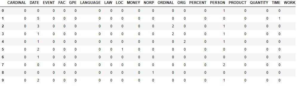
NER Analysis

Let’s perform Named Entity Recognition (NER) using spacy

nlp = spacy.load(“en_core_web_sm”)

def subj_obj_count(review):

sent = review
doc=nlp(sent)
sub_words = set([str(word) for word in doc if (word.dep_ == "nsubj")])

obj_words = set([str(word) for word in doc if (word.dep_ == "dobj")])

return len(sub_words),len(obj_words)

count = []

for r in tqdm(data[‘review’]):
count.append(subj_obj_count(r))

100%|██████████| 212106/212106 [41:58<00:00, 84.22it/s] 

sub_obj = pd.DataFrame(count,columns=[‘subj_count’,’obj_count’])
sub_obj.head(10)

sub_obj.to_csv(‘sub_obj.csv’,index=False)

sub_obj = pd.read_csv(‘sub_obj.csv’)
sub_obj.shape

(212106, 2)

ner_lst = nlp.pipe_labels[‘ner’]

def ner(review):

sent = review
doc=nlp(sent)
dic = {}.fromkeys(ner_lst,0)
for word in doc.ents:
    dic[word.label_]+=1

return dic

entity = pd.DataFrame([ner(r) for r in tqdm(data[‘cleaned_review’])])

100%|██████████| 212106/212106 [33:50<00:00, 104.47it/s]   

entity.to_csv(‘entities.csv’,index=False)

entity = pd.read_csv(‘entities.csv’)
print(entity.shape)
entity.head(10)

(212106, 18)

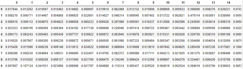
Topic Modelling

Topic Modelling in NLP analyzes the text data and finds the topics that best describes the set of documents. It is an Unsupervised approach as it recognizes and extracts the topics by detecting hidden patterns like clustering algorithms. Also it doesn’t require any predefined tags or training data.

Let’s pre-process the feature

corpus = data[‘cleaned_review’]

lst_corpus = []
for string in tqdm(corpus):
lst_words = string.split()
lst_grams = [” “.join(lst_words[i:i + 1]) for i in range(0, len(lst_words), 1)]
lst_corpus.append(lst_grams)

and map words to an id
id2word = gensim.corpora.Dictionary(lst_corpus)

while creating the dictionary word:freq
dic_corpus = [id2word.doc2bow(word) for word in lst_corpus]

Train LDA

Let’s train the LDA model

lda_model = gensim.models.ldamodel.LdaModel(corpus=dic_corpus, id2word=id2word, num_topics=20, chunksize=100, passes=10, alpha=’auto’, per_word_topics=True)

100%|██████████| 212106/212106 [00:02<00:00, 74286.58it/s]

storing the topic vectors for each review in a list

train_vecs = []
for i in range(len(corpus)):
top_topics = (
lda_model.get_document_topics(dic_corpus[i],
minimum_probability=0.0)
)
topic_vec = [top_topics[i][1] for i in range(20)]

train_vecs.append(topic_vec)

topics = pd.DataFrame(train_vecs)
print(topics.shape)
topics.head(10)

(212106, 20)

Let’s export this table to csv

topics.to_csv(‘topics.csv’,index=False)

Topic Correlations

Let’s read the topics data

topics = pd.read_csv(‘topics.csv’)
topics.shape

(212106, 20)

while concatenating sub_obj, entity and topics

data = pd.concat([data,sub_obj,entity,topics],axis=1)
print(data.shape)
data.tail(10)

(212106, 58)

Let’s calculate correlations as 53 rows × 53 columns

data.corr()

Let’s plot the corresponding correlation heatmap lower triangle with seaborn

corr2_data = data.corr(method=’pearson’)
mask_ut=np.triu(np.ones(corr2_data.shape)).astype(np.bool)

f, ax = plt.subplots(figsize=(22, 18))
sns.set(font_scale=1)
cmap = sns.diverging_palette(220, 10, as_cmap=True)

sns.heatmap(corr2_data, mask=mask_ut, cmap=”Spectral”,annot=True, annot_kws={“size”:6})
hmap.figure.savefig(“Correlation_Heatmap_topics_Lower_Triangle_with_Seaborn.png”,
format=’png’,
dpi=150)

Let’s export the newly processed data

data.to_csv(‘final_new_data_processed.csv’,index=False)

NLP Modelling

Finally, we are ready to build training models for classifying reviews. This would require the following libraries:

import pandas as pd
import numpy as np
import matplotlib.pyplot as plt
import seaborn as sns
import warnings
warnings.filterwarnings(‘ignore’)
from wordcloud import WordCloud
from wordcloud import STOPWORDS
import nltk
import regex as re

from nltk.corpus import stopwords
from nltk.stem.snowball import SnowballStemmer

Let’s read the data

data = pd.read_csv(‘final_new_data_processed.csv’)
print(data.shape)
data.head(10)

(212106, 58)

Let’s drop 5 unwanted columns

X = data.drop([‘uniqueID’,’review’,’rating’,’date’,’review_sentiment’],axis=1)
y = data[‘review_sentiment’].values
print(X.shape)

(212106, 53)

Let’s split our data into the 70% training and 30% test datasets while creating 21% cross-validation (CV) data using train_test_split

from sklearn.model_selection import train_test_split

X_train, X_test, y_train, y_test = train_test_split(X,y,stratify=y,test_size=0.30,random_state=42)

X_train, X_cv, y_train, y_cv = train_test_split(X_train, y_train,stratify=y_train,test_size=0.30,random_state=42)

print(‘Train data size is:’,X_train.shape)
print(‘Cross Validation data size is:’,X_cv.shape)
print(‘Test data size is:’,X_test.shape)

Train data size is: (103931, 53)
Cross Validation data size is: (44543, 53)
Test data size is: (63632, 53)

Let’s perform encoding Categorical, text and numerical features using LabelEncoder

from sklearn.preprocessing import LabelEncoder

lab_enc_cond = LabelEncoder()

lab_enc_cond.fit(X[‘condition’].values)

X_train_condition = lab_enc_cond.transform(X_train[‘condition’].values).reshape(-1,1)
X_test_condition = lab_enc_cond.transform(X_test[‘condition’].values).reshape(-1,1)
X_cv_condition = lab_enc_cond.transform(X_cv[‘condition’].values).reshape(-1,1)

print(‘After Encoding’)
print(‘Train data shape’,X_train_condition.shape)
print(‘Test data shape’,X_test_condition.shape)
print(‘CV data shape’,X_cv_condition.shape)

After Encoding
Train data shape (103931, 1)
Test data shape (63632, 1)
CV data shape (44543, 1)

Let’s export the condition encoder

import joblib
print(‘Saving condition encoder..’)
joblib.dump(lab_enc_cond,’condition_encoder.pkl’)

Saving condition encoder..

Out[95]:

['condition_encoder.pkl']

Let’s apply label encoder

lab_enc_year = LabelEncoder()

lab_enc_year.fit(X[‘year’].values)

X_train_year = lab_enc_year.transform(X_train[‘year’].values).reshape(-1,1)
X_test_year = lab_enc_year.transform(X_test[‘year’].values).reshape(-1,1)
X_cv_year = lab_enc_year.transform(X_cv[‘year’].values).reshape(-1,1)

print(‘After Encoding’)
print(‘Train data shape’,X_train_year.shape)
print(‘Test data shape’,X_test_year.shape)
print(‘CV data shape’,X_cv_year.shape)

After Encoding
Train data shape (103931, 1)
Test data shape (63632, 1)
CV data shape (44543, 1)

Let’s export the year encoder

print(‘Saving year encoder..’)
joblib.dump(lab_enc_year,’year_encoder.pkl’)

Saving year encoder..

Out[97]:

['year_encoder.pkl']

BoW Vectorizer

The text data can be encoded in different forms.

The ‘cleaned review’ text data can be vectorized using Bag of Words (BoW) as 1 gram tokens

from sklearn.feature_extraction.text import CountVectorizer,TfidfVectorizer
from sklearn.preprocessing import Normalizer,StandardScaler,MinMaxScaler
import joblib

vect_bow_1 = CountVectorizer(min_df=10,ngram_range=(1,1))

X_train1 = X_train.dropna()

vect_bow_1.fit(X_train1[‘cleaned_review’].values)

CountVectorizer(min_df=10)

X_train_review_bow_1 = vect_bow_1.transform(X_train1[‘cleaned_review’].values)

X_test1 = X_test.dropna()

X_test_review_bow_1 = vect_bow_1.transform(X_test1[‘cleaned_review’].values)

X_cv1=X_cv.dropna()

X_cv_review_bow_1 = vect_bow_1.transform(X_cv1[‘cleaned_review’].values)

print(‘After Vectorization’)
print(‘Train data shape:’,X_train_review_bow_1.shape)
print(‘Test data shape:’,X_test_review_bow_1.shape)
print(‘CV data shape:’,X_cv_review_bow_1.shape)

After Vectorization
Train data shape: (103927, 7294)
Test data shape: (63628, 7294)
CV data shape: (44543, 7294)

print(‘Vectorizer for BoW is saved..’)
joblib.dump(vect_bow_1,’vectorizer_bow.pkl’)

Vectorizer for BoW is saved..

Out[108]:

['vectorizer_bow.pkl']

TF-IDF Vectorizer

Let’s vectorize our cleaned review data using the Term Frequency and Inverse Document Frequency (TF-IDF) as 1 gram tokens fitted on training data only

vect_tfidf_1 = TfidfVectorizer(min_df=10,ngram_range=(1,1))

vect_tfidf_1.fit(X_train1[‘cleaned_review’].values)

X_train_review_tfidf_1 = vect_tfidf_1.transform(X_train1[‘cleaned_review’].values)
X_test_review_tfidf_1 = vect_tfidf_1.transform(X_test1[‘cleaned_review’].values)
X_cv_review_tfidf_1 = vect_tfidf_1.transform(X_cv1[‘cleaned_review’].values)

print(‘After Vectorization’)
print(‘Train data shape:’,X_train_review_tfidf_1.shape)
print(‘Test data shape:’,X_test_review_tfidf_1.shape)
print(‘CV data shape:’,X_cv_review_tfidf_1.shape)

After Vectorization
Train data shape: (103927, 7294)
Test data shape: (63628, 7294)
CV data shape: (44543, 7294)

print(‘Vectorizer for TF-IDF is saved..’)
joblib.dump(vect_tfidf_1,’vectorizer_tfidf.pkl’)

Word2Vec Vectorizer

The cleaned review text data is now vectorized using Word2Vec

from tqdm import tqdm
cleaned_reviews = data[‘cleaned_review’].values

In doing so, we need to import the pre-trained Glove model as glove.6B.300d.txt

def loadGloveModel(gloveFile):
print (“Loading Glove Model”)
f = open(gloveFile,’r’, encoding=”utf8″)
model = {}
for line in tqdm(f):
splitLine = line.split()
word = splitLine[0]
embedding = np.array([float(val) for val in splitLine[1:]])
model[word] = embedding
print (“Done.”,len(model),” words loaded!”)
return model
model = loadGloveModel(‘glove.6B.300d.txt’)

Loading Glove Model

400000it [00:34, 11432.30it/s]

Done. 400000  words loaded!

words = []
for i in cleaned_reviews:
words.extend(str(i).split(‘ ‘))

Let' check the number of words that are present in both glove vectors and our corpus

print(“all the words in the corpus”, len(words))
words = set(words)
print(“the unique words in the corpus”, len(words))

inter_words = set(model.keys()).intersection(words)
print(“The number of words that are present in both glove vectors and our corpus”, \
len(inter_words),”(“,np.round(len(inter_words)/len(words)*100,3),”%)”)

words_courpus = {}
words_glove = set(model.keys())
for i in words:
if i in words_glove:
words_courpus[i] = model[i]
print(“word 2 vec length”, len(words_courpus))

all the words in the corpus 8868702
the unique words in the corpus 34667
The number of words that are present in both glove vectors and our corpus 13620 ( 39.288 %)
word 2 vec length 13620

Let’s invoke the pickle binary protocol for serializing/de-serializing our vectors

import pickle
with open(‘glove_vectors’, ‘wb’) as f:
pickle.dump(words_courpus, f)

with open(‘glove_vectors’, ‘rb’) as f:
model = pickle.load(f)
glove_words = set(model.keys())
print(len(glove_words))

13620

Let’s create the list of columns

columns = [‘usefulCount’,’word_count’,’unique_word_count’,’char_length’,’count_punctuations’,’stopword_count’,
‘mean_word_len’,’subj_count’,’obj_count’,’CARDINAL’,’DATE’,’EVENT’,’FAC’,’GPE’,’LANGUAGE’,’LAW’,
‘LOC’,’MONEY’,’NORP’,’ORDINAL’,’ORG’, ‘PERCENT’,’PERSON’, ‘PRODUCT’,’QUANTITY’,’TIME’,’WORK_OF_ART’,
‘0’,’1′,’2′,’3′,’4′,’5′,’6′,’7′,’8′,’9′,’10’,’11’,’12’,’13’,’14’,’15’,’16’,’17’,’18’,’19’]

and apply Normalizer() to the train, test and CV data

normalizer = Normalizer()

X_train_num_1 = normalizer.fit_transform(X_train1[columns])
X_test_num_1 = normalizer.fit_transform(X_test1[columns])
X_cv_num_1 = normalizer.fit_transform(X_cv1[columns])

print(“After vectorizations”)
print(X_train_num_1.shape, y_train.shape)
print(X_test_num_1.shape, y_test.shape)
print(X_cv_num_1.shape, y_cv.shape)

After vectorizations
(103927, 47) (103931,)
(63628, 47) (63632,)
(44543, 47) (44543,)

Let’s create the subsets with sentiment_score and sentiment_score_clean values

X_train_sent_score = X_train1[[‘sentiment_score’,’sentiment_score_clean’]].values
X_test_sent_score = X_test1[[‘sentiment_score’,’sentiment_score_clean’]].values
X_cv_sent_score = X_cv1[[‘sentiment_score’,’sentiment_score_clean’]].values

print(“After vectorizations”)
print(X_train_sent_score.shape, y_train.shape)
print(X_test_sent_score.shape, y_test.shape)
print(X_cv_sent_score.shape, y_cv.shape)

After vectorizations
(103927, 2) (103931,)
(63628, 2) (63632,)
(44543, 2) (44543,)

Let’s concatenate all encoded features (all extracted features + sentiment scores)

from scipy.sparse import hstack
X_tr_1 = np.concatenate((X_train_num_1,X_train_sent_score),axis=1)

X_te_1 = np.concatenate((X_test_num_1,X_test_sent_score),axis=1)

X_cv_1 = np.concatenate((X_cv_num_1,X_cv_sent_score),axis=1)

print(“Final Data matrix”)
print(X_tr_1.shape, y_train.shape)
print(X_te_1.shape, y_test.shape)
print(X_cv_1.shape, y_cv.shape)

Final Data matrix
(103927, 49) (103931,)
(63628, 49) (63632,)
(44543, 49) (44543,)

NLP Modelling

We need a few performance metrics

from sklearn.metrics import log_loss, accuracy_score,confusion_matrix, f1_score,roc_auc_score,roc_curve

and the following functions

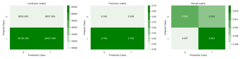
def plot_confusion_matrix(test_y, predict_y):
C = confusion_matrix(test_y, predict_y)
print(“Number of misclassified points “,(len(test_y)-np.trace(C))/len(test_y)*100)

A =(((C.T)/(C.sum(axis=1))).T)

B =(C/C.sum(axis=0))

plt.figure(figsize=(20,4))

labels = [0,1]
cmap=sns.light_palette("green")
plt.subplot(1, 3, 1)
sns.heatmap(C, annot=True, cmap=cmap, fmt=".3f", xticklabels=labels, yticklabels=labels)
plt.xlabel('Predicted Class')
plt.ylabel('Original Class')
plt.title("Confusion matrix")

plt.subplot(1, 3, 2)
sns.heatmap(B, annot=True, cmap=cmap, fmt=".3f", xticklabels=labels, yticklabels=labels)
plt.xlabel('Predicted Class')
plt.ylabel('Original Class')
plt.title("Precision matrix")

plt.subplot(1, 3, 3)
sns.heatmap(A, annot=True, cmap=cmap, fmt=".3f", xticklabels=labels, yticklabels=labels)
plt.xlabel('Predicted Class')
plt.ylabel('Original Class')
plt.title("Recall matrix")

plt.show()    

def model_metrics(clf,train_data,test_data,cv_data):

print('**LogLoss**')
predict_y = clf.predict_proba(train_data)
print ("The train log loss is:",log_loss(y_train, predict_y))
predict_y = clf.predict_proba(cv_data)
print( "The cross validation log loss is:",log_loss(y_cv, predict_y))
predict_y = clf.predict_proba(test_data)
print( "The test log loss is:",log_loss(y_test, predict_y))

print(50*'-')

print('**Accuracy**')
y_pred_tr = clf.predict(train_data)
print ("The train Accuracy is:",accuracy_score(y_train, y_pred_tr))
y_pred_cv = clf.predict(cv_data)
print( "The cross validation Accuracy is:",accuracy_score(y_cv, y_pred_cv))
y_pred_te = clf.predict(test_data)
print( "The test Accuracy is:",accuracy_score(y_test, y_pred_te))

print(50*'-')


print('**F1 Score**')    
print ("The train F1 score is:",f1_score(y_train, y_pred_tr))
print( "The cross validation F1 score is:",f1_score(y_cv, y_pred_cv))
print( "The test F1 score is:",f1_score(y_test, y_pred_te))

print(50*'-')

print('**AUC**')   
print ("The train AUC is:",roc_auc_score(y_train, y_pred_tr))
print( "The cross validation AUC is:",roc_auc_score(y_cv, y_pred_cv))
print( "The test AUC is:",roc_auc_score(y_test, y_pred_te))

print(50*'-')

As an example, let’s deploy the Random Model
test_len = len(y_test)
predicted_y = np.zeros((test_len,2))
for i in range(test_len):
rand_probs = np.random.rand(1,2)
predicted_y[i] = ((rand_probs/sum(sum(rand_probs)))[0])
print(“Log loss on Test Data using Random Model”,log_loss(y_test, predicted_y, eps=1e-15))

predicted_y =np.argmax(predicted_y, axis=1)

print(“Accuray on Test Data using Random Model”,accuracy_score(y_test, predicted_y))
print(“F1 score on Test Data using Random Model”,f1_score(y_test, predicted_y))
print(“AUC on Test Data using Random Model”,roc_auc_score(y_test, predicted_y))

Log loss on Test Data using Random Model 0.8817010788104614
Accuray on Test Data using Random Model 0.5019644204174001
F1 score on Test Data using Random Model 0.5859171860504618
AUC on Test Data using Random Model 0.5014991363225234

plot_confusion_matrix(y_test,predicted_y)
plt.show()
plt.savefig(‘drugsconfmatrix.png’)

Number of misclassified points  49.80355795826

Conclusion

Following recent ML and DA studies, we have addressed the problem of building an NLP-based drug recommendation system in Python. It appears that the Sentiment Analysis, Topic Modelling and Word2Vec techniques play a major role in classifying the drug reviews thereby recommending the effective drugs.

The simplest way to deploy our trained LDA model is to create a web service using the Flask web framework. A final web app can be deployed within the multi-cloud environment discussed in Appendix.

Appendix:

Multi-Cloud NLP Drug Recommendation

AWS:

One can use Amazon Comprehend Medical to extract medication names and medical conditions to monitor drug safety and adverse events. Amazon Comprehend Medical is a NLP service that uses AI to easily extract relevant medical information from unstructured text. We query the OpenFDA API (an open-source API published by the FDA) and Clinicaltrials.gov API (another open-source API published by the National Library of Medicine (NLM) at the National Institutes of Health (NIH)) to get information on past adverse events, recalls, and clinical trials for the drug or medical condition in question. One can then use this data in population scale studies to further analyze the drug’s safety and efficacy.

GCP

Several successful case studies can guide you through the process of creating an ERC20 token recommendation system built with TensorFlow, Cloud Machine Learning Engine, Cloud Endpoints, and App Engine created at Google Cloud. The key point is the collaborative filtering technique for generating user recommendations. Collaborative filtering relies only on observed user behavior to make recommendations — no profile data or content access is necessary. The entire workflow looks like this:

• Creating and training the model for token recommendation system
• Query token ratings from BigQuery
• Train the model locally and in Google ML Engine
• Tuning hyperparameters in Cloud ML Engine
• Deploying the recommendation system to Google App Engine

With the development of e-commerce, a growing number of people prefer to purchase medicine online. To provide online medication guidance, the novel cloud-assisted drug recommendation system CADRE can recommend users with top-N related medicines according to symptoms.

Azure

Healthcare organizations are using Azure products and services—including hybrid cloud, mixed reality, AI, and IoT—to drive better health outcomes, improve security, scale faster, and enhance data interoperability.

Text Analytics is now Azure Language Service. Specifically, Sentiment Analysis and Opinion Mining, Named Entity Recognition (NER), Entity Linking, Key Phrase Extraction, Language Detection, Text Analytics for health, and Text Summarization are all part of the Language Service as they exist today. 

Using the Text Analytics NER, users can extract known types like person names, geographical locations, datetimes, and organizations. However, lots of information of interest is more specific than the standard types. The capability allows you to build your own custom entity extractors by providing labelled examples of text to train models.