A medication recommender framework is truly vital with the goal that it can assist specialists and help patients to build their knowledge of drugs on specific health conditions [1-4].
Contents:
- Workflow
- Importing Libraries
- Read Raw Data
- Data Content
- Plotting Top 10 Conditions
- Drug Count for Each Condition
- Top 10 Drugs Used for the Top Condition
- Plotting Top 10 Drugs Rated as 10
- Plotting Top 10 Drugs Rated as 1
- Plotting Percentage of Ratings using Pie Chart
- Distribution of usefulCount Feature
- Distribution of Ratings
- Summary
- References

Objective: Build a Drug Recommendation System that recommends the most effective drug for a certain condition based on available reviews of various drugs used to treat this condition.
The Kaggle UCI ML Drug Review dataset provides over 200000 patient reviews on specific drugs along with related conditions and a 10-star patient rating system reflecting overall patient satisfaction. The data was obtained by crawling online pharmaceutical review sites [1]. This data was published in a study on sentiment analysis of drug experience over multiple facets, ex. sentiments learned on specific aspects such as effectiveness and side effects.
The input dataset contains 7 columns: uniqueID, drugName, condition, review, rating, date, and usefulCount.
Workflow
- Importing relevant libraries
- Reading input raw data
- Check data content/statistics
- Plotting top 10 conditions
- Drug count for each condition
- Top 10 drugs used for the top condition
- Plotting the top 10 drugs rated as 1 or 10
- Plotting the percentage distribution of ratings using pie chart
- Checking the distribution of usefulCount feature
- Data analytics report summary
Importing Libraries
Let’s set the working directory YOURPATH
import os
os.chdir(‘YOURPATH’) # Set working directory
Let’s import libraries
import pandas as pd
import numpy as np
import matplotlib.pyplot as plt
import seaborn as sns
from mlxtend.plotting import plot_decision_regions
plt.style.use(‘ggplot’)
%config InlineBackend.figure_format = ‘svg’
%matplotlib inline
np.set_printoptions(suppress=True)
!pip install nltk
import re # Regular expression library
import string
import nltk
from nltk.corpus import stopwords
from nltk.stem.snowball import SnowballStemmer
from nltk.stem import WordNetLemmatizer
from nltk.tokenize import word_tokenize
nltk.download(‘stopwords’)
nltk.download(‘wordnet’)
nltk.download(‘punkt’)
!pip install spacy
!python -m spacy download en_core_web_sm
Read Raw Data
and read the input train and test datasets
df_train = pd.read_csv(‘drugsComTrain_raw.csv’)
df_test = pd.read_csv(‘drugsComTest_raw.csv’)
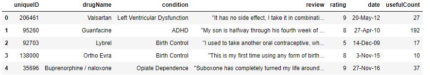
print(‘Overview of Train dataset:\n’)
df_train.head(5)
Overview of Train dataset:
Similarly,
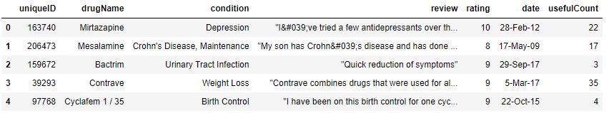
print(‘Overview of Test dataset:\n’)
df_test.head(5)
Overview of Test dataset:
Data Content
Let’s look at the training data summary info
df_train.info()
<class 'pandas.core.frame.DataFrame'>
RangeIndex: 161297 entries, 0 to 161296
Data columns (total 7 columns):
 #   Column       Non-Null Count   Dtype
---  ------       --------------   -----
 0   uniqueID     161297 non-null  int64
 1   drugName     161297 non-null  object
 2   condition    160398 non-null  object
 3   review       161297 non-null  object
 4   rating       161297 non-null  int64
 5   date         161297 non-null  object
 6   usefulCount  161297 non-null  int64
dtypes: int64(3), object(4)
memory usage: 8.6+ MB
Let’s check the dimensions of these two datasets
data_train.shape
(161297, 7)
data_test.shape
(53766, 7)
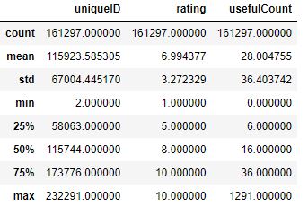
let’s look at the descriptive statistics of the training dataset
df_train.describe()
Let’s check for missing values
df_train.isnull().any()
uniqueID       False
drugName       False
condition       True
review         False
rating         False
date           False
usefulCount    False
dtype: bool
and calculate the percentage of missing values
percent_missing = df_train.isnull().sum() * 100 / len(df_train)
print(percent_missing)
uniqueID       0.000000
drugName       0.000000
condition      0.557357
review         0.000000
rating         0.000000
date           0.000000
usefulCount    0.000000
dtype: float64
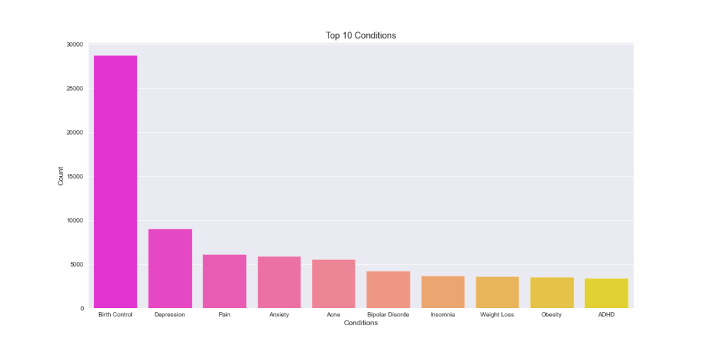
Plotting Top 10 Conditions
data=df_train
conditions = dict(data[‘condition’].value_counts())
top_conditions = list(conditions.keys())[0:10]
values = list(conditions.values())[0:10]
plt.figure(figsize=(16,8))
sns.set_style(style=’darkgrid’)
sns.barplot(x=top_conditions,y=values,palette=’spring’)
plt.title(‘Top 10 Conditions’)
plt.xlabel(‘Conditions’)
plt.ylabel(‘Count’)
plt.show()
plt.savefig(‘conditionstop10.png’)
Drug Count for Each Condition
val=[]
for c in list(conditions.keys()):
val.append(data[data[‘condition’]==c][‘drugName’].nunique())
drug_cond = dict(zip(list(conditions.keys()),val))
top_conditions = list(drug_cond.keys())[0:10]
values = list(drug_cond.values())[0:10]
plt.figure(figsize=(16,8))
sns.set_style(style=’darkgrid’)
sns.barplot(x=top_conditions,y=values,palette=’spring’)
plt.title(‘Number of Drugs for each Top 10 Conditions’)
plt.xlabel(‘Conditions’)
plt.ylabel(‘Count of Drugs’)
plt.show()
plt.savefig(‘drugcounttop10.png’)

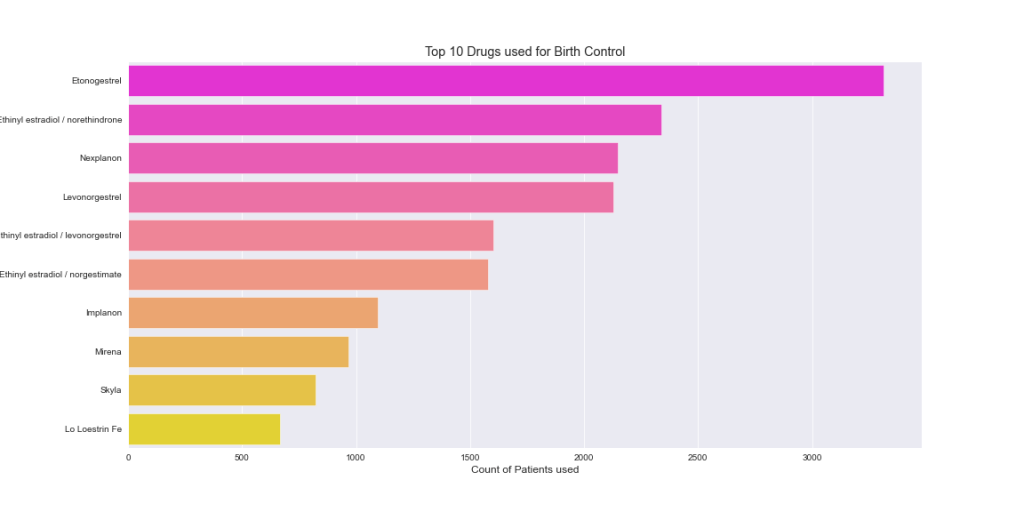
Top 10 Drugs Used for the Top Condition
drugs_birth = dict(data[data[‘condition’]==’Birth Control’][‘drugName’].value_counts())
top_drugs = list(drugs_birth.keys())[0:10]
values = list(drugs_birth.values())[0:10]
plt.figure(figsize=(16,8))
sns.set_style(style=’darkgrid’)
sns.barplot(x=values,y=top_drugs,palette=’spring’)
plt.title(‘Top 10 Drugs used for Birth Control’)
plt.ylabel(‘Drug Names’)
plt.xlabel(‘Count of Patients used’)
plt.show()
plt.savefig(‘drugcountbirthcontrol.png’)
Plotting Top 10 Drugs Rated as 10
drugs_rating = dict(data[data[‘rating’]==10][‘drugName’].value_counts())
top_drugs = list(drugs_rating.keys())[0:10]
values = list(drugs_rating.values())[0:10]
plt.figure(figsize=(16,8))
sns.set_style(style=’darkgrid’)
sns.barplot(x=values,y=top_drugs,palette=’spring’)
plt.title(‘Top 10 Drugs rated as 10’)
plt.ylabel(‘Drug Names’)
plt.xlabel(‘Count of Ratings’)
plt.show()
plt.savefig(‘drugstop10rate10.png’)

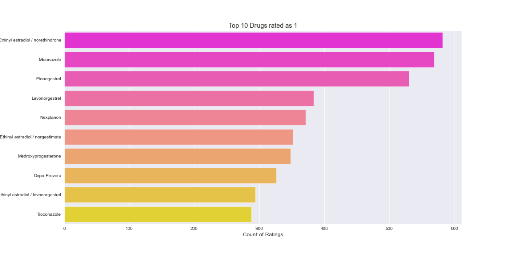
Plotting Top 10 Drugs Rated as 1
drugs_rating = dict(data[data[‘rating’]==1][‘drugName’].value_counts())
top_drugs = list(drugs_rating.keys())[0:10]
values = list(drugs_rating.values())[0:10]
plt.figure(figsize=(16,8))
sns.set_style(style=’darkgrid’)
sns.barplot(x=values,y=top_drugs,palette=’spring’)
plt.title(‘Top 10 Drugs rated as 1’)
plt.ylabel(‘Drug Names’)
plt.xlabel(‘Count of Ratings’)
plt.show()
plt.savefig(‘drugstop10rate1.png’)
Plotting Percentage of Ratings using Pie Chart
ratings_count = dict(data[‘rating’].value_counts())
count = list(ratings_count.values())
labels = list(ratings_count.keys())
plt.figure(figsize=(18,9))
plt.pie(count,labels=labels, autopct=’%1.1f%%’)
plt.title(‘Pie Chart Representation of Ratings’)
plt.legend(title=’Ratings’)
plt.show()
plt.savefig(‘drugsratingsall.png’)

Distribution of usefulCount Feature
plt.figure(figsize=(16,8))
ax =sns.distplot(data[‘usefulCount’])
plt.title(‘Distribution of usefulCount’)
plt.show()
plt.savefig(‘drugsusefulcontent.png’)

Distribution of Ratings
f,ax = plt.subplots(1,2,figsize=(16,8))
ax1= sns.histplot(data[‘rating’],ax=ax[0])
ax1.set_title(‘Count of Ratings’)
ax2= sns.distplot(data[‘rating’],ax=ax[1])
ax2.set_title(‘Distribution of Ratings Density’)
plt.show()
plt.savefig(‘distributionratingsdens.png’)

Summary
- The categorical feature condition has 0.55% missing values to be dropped.
- Birth Control is the topmost condition followed by Depression, Pain, and Anxiety.
- Patients use several drugs to treat their conditions.
- Pain and Birth Control conditions have the highest drug count.
- Top drugs used for Birth Control are Etonogestrel Ethinyl Estradiol, Levonorgestrel and Nexplanon.
- Birth Control and Weight Loss/Obesity drugs are top rated.
- Etonogestrel and Levonorgestrel should be the top 2 recommended drugs as they are mostly frequently used and also rated as 10.
- It appears that ~75% of drugs are rated with 10,9,8 and 1 ratings.
- The maximum number of drug reviews is less than 200 upvotes.
References
The dataset was originally published on the UCI Machine Learning repository. Citation:
[1] Felix Gräßer, Surya Kallumadi, Hagen Malberg, and Sebastian Zaunseder. 2018. Aspect-Based Sentiment Analysis of Drug Reviews Applying Cross-Domain and Cross-Data Learning. In Proceedings of the 2018 International Conference on Digital Health (DH ’18). ACM, New York, NY, USA, 121-125.
[2] Sumit Mishra 2020 Python code
[3] Ruthvik Marshetty Drug Recommendation System: Medium June 4, 2022. Ref.
Github Repository, Research paper Garg (2021)
[4] Github jisong316


Leave a comment