Stock Forecasting with FBProphet

Contents:

1. Introduction
2. Installations
   1. #To activate this environment, use
   2. #conda activate stan_env
   3. #To deactivate an active environment, use
   4. #conda deactivate
3. Predictions
4. Comments
5. Summary
6. References

Introduction

Facebook Prophet is open-source library released by Facebook’s Core Data Science team. It is available in R and Python. Prophet is a procedure for univariate (one variable) time series forecasting data based on an additive model, and the implementation supports trends, seasonality, and holidays. It works best with time series that have strong seasonal effects and several seasons of historical data. Prophet is robust to missing data and shifts in the trend, and typically handles outliers well.

See References below.

Installations

Let’s install Anaconda IDE and set up the appropriate Conda environment

cd ~\anaconda3\condabin

conda info

conda update conda

#To activate this environment, use

#conda activate stan_env

#To deactivate an active environment, use

#conda deactivate

conda activate stan_env

conda install libpython m2w64-toolchain -c msys2

conda install numpy cython -c conda-forge

conda install matplotlib scipy pandas -c conda-forge

conda install pystan -c conda-forge

conda install -c anaconda ephem

conda install -c conda-forge fbprophet

Let’s open the Jupyter notebook and install the following libraries within stan_env

!pip install yfinance

import yfinance as yf

!pip install chart_studio

import pandas as pd
import numpy as np
import scipy as sp
import chart_studio.plotly as py

from fbprophet import Prophet

Predictions

We read historical stock data using Yahoo Finance. For example, let’s look at AMZN

stock_ticker = ‘AMZN’
yfin = yf.Ticker(stock_ticker)
hist = yfin.history(period=”max”)
hist = hist[[‘Close’]]
hist.reset_index(level=0, inplace=True)
hist = hist.rename({‘Date’: ‘ds’, ‘Close’: ‘y’}, axis=’columns’)
m = Prophet(daily_seasonality=True)
m.fit(hist)

future = m.make_future_dataframe(periods=365)
forecast = m.predict(future)
pd.options.display.max_columns = None
print(forecast.tail(2))

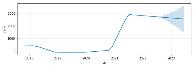
ds       trend   yhat_lower   yhat_upper  trend_lower  \
6669 2023-06-02  4078.16732  3849.983952  4234.406491  4062.805046   
6670 2023-06-03  4079.59198  3858.633118  4244.843251  4064.126297   

      trend_upper  additive_terms  additive_terms_lower  additive_terms_upper  \
6669  4094.250080      -27.515668            -27.515668            -27.515668   
6670  4095.713544      -20.885808            -20.885808            -20.885808   

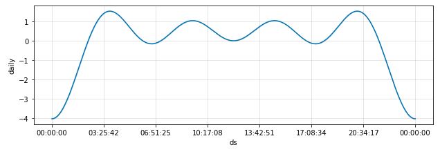
         daily  daily_lower  daily_upper    weekly  weekly_lower  \
6669 -4.041229    -4.041229    -4.041229 -2.170906     -2.170906   
6670 -4.041229    -4.041229    -4.041229  0.505153      0.505153   

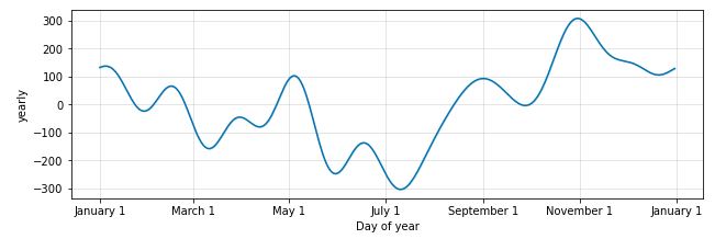
      weekly_upper     yearly  yearly_lower  yearly_upper  \
6669     -2.170906 -21.303533    -21.303533    -21.303533   
6670      0.505153 -17.349732    -17.349732    -17.349732   

      multiplicative_terms  multiplicative_terms_lower  \
6669                   0.0                         0.0   
6670                   0.0                         0.0   

      multiplicative_terms_upper         yhat  
6669                         0.0  4050.651652  
6670                         0.0  4058.706171  

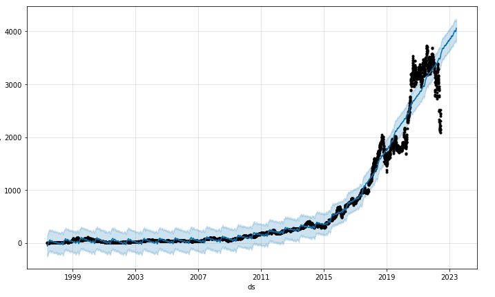
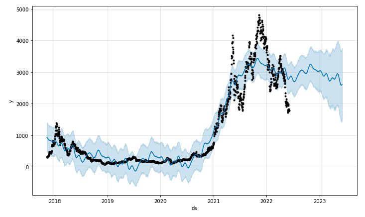
print(forecast[[‘ds’, ‘yhat’, ‘yhat_lower’, ‘yhat_upper’]].tail())

 ds         yhat   yhat_lower   yhat_upper
6666 2023-05-30  4037.772562  3842.484407  4226.067427
6667 2023-05-31  4043.137454  3847.566906  4241.015891
6668 2023-06-01  4047.812058  3841.219833  4243.001044
6669 2023-06-02  4050.651652  3849.983952  4234.406491
6670 2023-06-03  4058.706171  3858.633118  4244.843251

figure1 = m.plot(forecast)
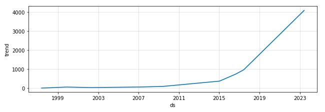
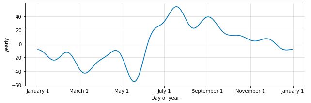
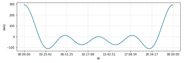
figure2 = m.plot_components(forecast)

Let’s apply the function

def predict(ticker,days):
yfin = yf.Ticker(ticker)
print(“Stock: “, yfin.info[‘name’])
hist = yfin.history(period=”max”)
hist = hist[[‘Close’]]
hist.reset_index(level=0, inplace=True)
hist = hist.rename({‘Date’: ‘ds’, ‘Close’: ‘y’}, axis=’columns’)
print(“Curent Data”)
print(hist.tail())
m = Prophet(daily_seasonality=True)
m.fit(hist)
future = m.make_future_dataframe(periods=days)
forecast = m.predict(future)
print(“Predicted Data”)
print(forecast[[‘ds’, ‘yhat’, ‘yhat_lower’, ‘yhat_upper’]].tail())
figure1 = m.plot(forecast)
figure2 = m.plot_components(forecast)

to the ETH-USD stock

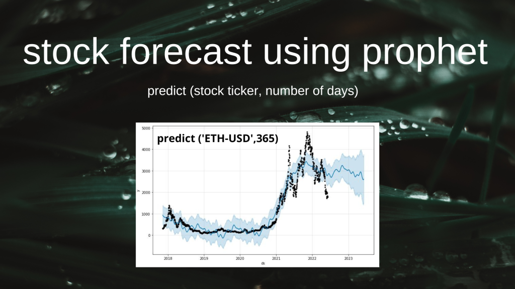
predict(“ETH-USD”,365)

Stock:  Ethereum
Curent Data
             ds            y
1665 2022-06-01  1823.569336
1666 2022-06-02  1834.150513
1667 2022-06-03  1775.078613
1668 2022-06-04  1801.609497
1669 2022-06-05  1784.663208
Predicted Data
             ds         yhat   yhat_lower   yhat_upper
2030 2023-06-01  2582.743017  1444.113747  3676.835993
2031 2023-06-02  2580.967269  1406.940449  3641.467382
2032 2023-06-03  2590.692980  1542.385844  3718.909670
2033 2023-06-04  2599.084116  1497.965969  3772.736086
2034 2023-06-05  2609.541418  1444.553404  3732.228581

For comparison, let’s look at BTC-USD

predict(“BTC-USD”,365)

Stock:  Bitcoin
Curent Data
             ds             y
2814 2022-06-01  29799.080078
2815 2022-06-02  30467.488281
2816 2022-06-03  29704.390625
2817 2022-06-04  29832.914062
2818 2022-06-05  29661.175781
Predicted Data
             ds          yhat    yhat_lower    yhat_upper
3179 2023-06-01  62526.361633  53359.687572  71979.300304
3180 2023-06-02  62678.484615  52661.381831  71895.027878
3181 2023-06-03  62855.408456  52764.612352  73328.871401
3182 2023-06-04  63017.050166  53448.588579  72521.046230
3183 2023-06-05  63261.548650  53875.600863  73277.660442

Comments

• Time series forecasting is one of most demanding object in machine learning. The easiest way for projecting your time series data is using a module named Prophet (aka fbprophet). This is a procedure for forecasting time series data based on an additive model where non-linear trends are fit with yearly, weekly, and daily seasonality, plus holiday effects.

• Prophet follows the sklearn model API. We create an instance of the Prophet class and then call its fit and predict methods. We fit the model by instantiating a new Prophet object. Any settings to the forecasting procedure are passed into the constructor. Then you call its fit method and pass in the historical dataframe. Fitting should take 1-5 seconds.

• By default, Prophet uses a linear model for its forecast. When forecasting growth, there is usually some maximum achievable point: total market size, total population size, etc. This is called the carrying capacity, and the forecast should saturate at this point.

• Prophet allows you to make forecasts using a logistic growth trend model, with a specified carrying capacity.

• Prophet will only work for Python < 3.9. We need to build a new environment in Anaconda. This environment will only focus on time series forecasting using fbprophet. Don’t forget to add anaconda python path into environment variable inside Windows system Path.
• You can plot the forecast by calling the Prophet.plot method and passing in your forecast dataframe.

Summary

We have implemented fbprophet assisted stock prediction in Python by applying the function predict(stock ticker, number of days) to stocks AMZN, ETH-USD and BTC-USD while importing historical stock data from Yahoo Finance.

References

Hareesh Pallathoor Balakrishnan (2021) Stock Prediction using Prophet (Python).

Handhika Yanuar Pratama (2021) Installing FBProphet/Prophet for Time Series Forecasting in Jupyter Notebook.

GitHub Prophet Documentation – Quick Start.

StackOverflow: Installing fbprophet Python on Windows 10

PyStan on Windows

Plotly Graphing Libraries

Mitchell Krieger (2021) Time Series Analysis with Facebook Prophet: How it works and How to use it.