
- The objective of this study is to address the problem of real-time object tracking with low signal/noise ratios.
- We consider an object moving in 1D, 2D and 3D. We assume that we observe a noisy version of its location and speed at each time step. We want to track the object and possibly forecast its future motion.
- Many different algorithms have been proposed for object tracking. The Kalman Filter (KF) is one of most popular estimation algorithms that plays a critical role in many practical applications of computer vision (guidance, navigation, control of vehicles, robotics, surveillance monitoring, etc.).
- At its heart, the KF is a method of combining noisy (and possibly missing) measurements and predictions of the state of an object to achieve an estimate of its true current state. Measurement noise is assumed to follow a zero mean Gaussian probability density function.
- In principle, a KF method can estimate the position and velocity of the target along with the measurement noise covariance at each time step.
- In this article, we examine several methods of synthesizing KF, robust with respect to data outliers.
Table of Contents
- Setting the working directory YOURPATH
import os
os.chdir('YOURPATH')    # Set working directory
os. getcwd()
1D Analysis
- Let’s consider a radar tracking navigation system implemented as the 1D Kalman Filter. Each (position-time) simulation consists of 100 measurement points: the first state (position) versus the second state (velocity). This is a 1D motion considering a piecewise constant white noise acceleration model. The time sampling interval is 1 sec.
- The value Q=0 means no change is observed over time in velocity vs time because the process noise is equal to 0 while the variance of measurement noise is equal to 1.
- The values Q=1, 9 indicate that the measured states are almost similar to the true states.
- The numerical simulation function
'''
This function generates the data for a 1D motion considering a
Piecewise constant, white noise acceleration model, equation (14)

var_q is the variance of the process noise
R is the variance of measurement noise
z is the measured data
x are the true values of the system states


'''

import sys
import numpy as np
import matplotlib.pyplot as plt

R = float('50')
N = 100 # data size
T = 1.0 # [s] Sampling time interval
A = np.array([[1, T],
              [0, 1]], dtype=float)  # Transition matrix

def simulate(var_q):
    var_q = float(var_q)
    x = np.zeros((2, N)) # states are [position; speed; acceleration]
    x[:, 0] = [0, 10] # state initialization, change to give your own initial values
    G = np.array([[T**2/2],
                  [T]], dtype=float) # Vector gain for the process noise
    w = np.random.normal(0.0, np.sqrt(var_q), N) # process noise
    for ii in range(1, N): # simulate system dynamics
      x[:, ii] = A.dot(x[:, ii-1]) + G.dot(w[ii]).T

    v = np.random.normal(0.0, np.sqrt(R), N) # measurement noise
    z = x[0, :] + v  # position measurements assuming C = [1 0 ]

    f1 = plt.figure()
    plt.plot(z, label='linear')
    plt.xlabel('Time [s]')
    plt.ylabel('Measured position')

    f2 = plt.figure()
    plt.plot(x[0,:], label='linear')
    plt.xlabel('Time [s]')
    plt.ylabel('True position [m]')

    f3 = plt.figure()
    plt.plot(x[1,:], label='linear')
    plt.xlabel('Time [s]')
    plt.ylabel('True speed [m/s]')

    return var_q, x, G, w, z
- Implementing the 1D Kalman Filter
import pandas as pd
import numpy as np
import matplotlib.pyplot as plt
%matplotlib inline

#t_states is true states
def apply_kf(t_states,z,R,var_q):
    NEES = np.zeros(N)
    NIS = np.zeros(N)
    S = np.zeros(N)
    # initial variables
    x = np.zeros((N+1,2,1))
    x[0][0][0]=z[0]
    x[0][0][0]=(z[1]-z[0])/T

    k = np.zeros((N,2,1))
    u = np.zeros(N)
    v = 0
    C = np.array(np.mat('1 0'))
    B = np.zeros((2,1))
    _p = np.zeros((N+1,2,2))

    #covariance
    p = np.zeros((N+1,2,2))
    init_p=np.array([[R,R/T],
                 [R/T,2*R/(T**2)]])
    # calculate the inverse of initial covariance matrix.
    p[0]=np.linalg.inv(init_p)

    for i in range(0,N):
        #Eq 5
        x[i+1] = A.dot(x[i]) + B.dot(u[i])
        #Eq 6
        _p[i] = A.dot(p[i]).dot(A.T) + G.dot(var_q).dot(G.T)
        #(Eq 7) Compute the Kalman gain
        k[i] = (_p[i].dot(C.T))/(np.dot(C.dot(_p[i]),C.T) + R)

        #Update the estimate and the error covariance
        #Eq 8
        x[i+1] = x[i+1]+k[i]*(z[i]-np.dot(C,x[i+1]))
        #Eq 9
        p[i+1] = np.dot(1-np.dot(k[i],C),_p[i])

        x_diff = np.reshape(t_states[:, i], (2,1))-x[i+1]
        NEES[i] = np.dot(np.dot(x_diff.T,np.linalg.inv(p[i+1])),x_diff)
        S[i] = np.dot(np.dot(C,_p[i]),C.T)+R
        temp = z[i]-np.dot(C,x[i+1])
        NIS[i] = temp**2/S[i]
    return NEES,NIS,k,p,_p,x
- Setting Q=1
(NEES,NIS,k,p,_p,_x) = apply_kf(x, z, R, float('1'))
plt.plot(_x[:,0],'r',linestyle='-',label='Estimated position')
plt.plot(x[0,:],'b', label='True position')
plt.xlabel('Time [s]')
plt.ylabel('Position [m]')
plt.title('Q = 1')
plt.legend()
plt.show()

plt.plot(_x[:,1],'r',label='Estimated speed')
plt.plot(x[1,:],'b', label='True speed')
plt.xlabel('Time [s]')
plt.ylabel('Velocity[m/s]')
plt.title('Q = 1')
plt.legend()
plt.show()

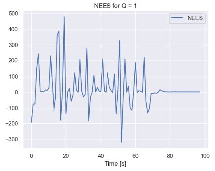
plt.plot(NEES[2::],label='NEES')
plt.title('NEES for Q = 1')
plt.xlabel('Time [s]')
plt.legend()
plt.show()
plt.plot(NIS[0::],label='NIS')
plt.title('NIS for Q = 1')
plt.xlabel('Time [s]')
plt.legend()
plt.show()

- The Kalman Filter for a linear position-time function with noisy velocity is given by
import numpy as np
from numpy.linalg import inv
import matplotlib.pyplot as plt

firstRun = True
x, P = np.array([[0,0]]).transpose(), np.zeros((2,2)) # X : Previous State Variable Estimation, P : Error Covariance Estimation
A, H = np.array([[0,0], [0,0]]), np.array([[0,0]])
Q, R = np.array([[0,0], [0,0]]), 0

def IntKalman(z):
    global firstRun
    global A, Q, H, R
    global x, P
    if firstRun:
        dt = 0.1
        A, Q = np.array([[1, dt], [0, 1]]), np.array([[1, 0], [0, 3]])
        # H, R = np.array([[1, 0]]),  np.array([10])
        H, R = np.array([[0, 1]]),  np.array([10])

        x = np.array([0, 80]).T
        P = 5 * np.eye(2)
        firstRun = False
    else:
        x_pred = A@x                              # x_pred : State Variable Prediction
        P_pred = A@P@A.T + Q                      # Error Covariance Prediction
        K = (P_pred@H.T) @ inv(H@P_pred@H.T + R)  # K : Kalman Gain
        x = x_pred + K@(z - H@x_pred)             # Update State Variable Estimation
        P = P_pred - K@H@P_pred                   # Update Error Covariance Estimation
    return x

# ------ Test program

np.random.seed(666)
Posp, Velp = None, None
def getVel(): #getPosSensor():
    global Posp, Velp
    if Posp == None:
        Posp = 0
        Velp = 80
    dt = 0.1

    # w = 0 + 10 * np.random.normal()
    v = 0 + 10 * np.random.normal()

    # z = Posp + Velp * dt + v  # Position measurement
    # Posp = z - v
    # Velp = 80 + w

    Posp = Posp + (Velp * dt)  # Position measurement
    z = Velp
    Velp = 80 + v
    print(f"v=>{v}")
    return z, Posp, Velp


time = np.arange(0, 10, 0.1)
Nsamples = len(time)

X_esti  = np.zeros([Nsamples, 2])
Z_saved = np.zeros([Nsamples, 2])

for i in range(Nsamples):
    Z, pos_true, vel_true = getVel()
    pos, vel = IntKalman(Z)

    X_esti[i]  = [pos, vel]
    Z_saved[i] = [pos_true, vel_true]

plt.figure()
plt.plot(time, Z_saved[:,1], 'b.', label = 'Measurements')
plt.plot(time, X_esti[:,1],  'r-', label='Kalman Filter')
plt.legend(loc='upper left')
plt.ylabel('Velocity [m/s]')
plt.xlabel('Time [sec]')

plt.figure()
plt.plot(time, Z_saved[:,0], 'b--', label='True Speed')
plt.plot(time, X_esti[:,0], 'r-', label='Kalman Filter')
plt.legend(loc='upper left')
plt.ylabel('Position [m]')
plt.xlabel('Time [sec]')
plt.show()

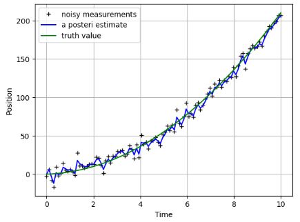
- Examining the Kalman Filter for the non-linear position-time function with noise
import numpy as np
import matplotlib.pyplot as plt
n=100
sz = (n) # size of array
t = np.linspace(0,10,n)
x = t + 2*t**2 # truth function
z = x + np.random.normal(0,7.5,size=sz) # noise

Q = 1e-3 # process variance

# allocate space for arrays
xhat=np.zeros(sz)      # a posteri estimate of x
P=np.zeros(sz)         # a posteri error estimate
xhatminus=np.zeros(sz) # a priori estimate of x
Pminus=np.zeros(sz)    # a priori error estimate
K=np.zeros(sz)         # Kalman gain

R = 0.03**2 # estimate of measurement variance


xhat[0] = 0.0
P[0] = 1.0

for i in range(1,n):

  xhatminus[i] = xhat[i-1]
  Pminus[i] = P[i-1]+Q


  K[i] = Pminus[i]/( Pminus[i]+R )
  xhat[i] = xhatminus[i]+K[i]*(z[i]-xhatminus[i])
  P[i] = (1-K[i])*Pminus[i]

plt.figure()
plt.plot(t, z,'k+',label='noisy measurements')
plt.plot(t, xhat,'b-',label='a posteri estimate')
plt.plot(t,x,color='g',label='truth value')
plt.legend()
plt.xlabel('Time')
plt.ylabel('Position')
plt.grid()

plt.show()
2D Analysis
- Let’s test the Sensor Fusion Kalman and the Particle 2D Filter. First, The trajectory of a single ball is predicted using the Kalman Filter. Then a particle filter is used to predict the trajectory of two balls simultaneously. The source code is based on the Recursive Density Estimation method.
- 2D Kalman Filter (KF) Class
import numpy as np
import matplotlib.pyplot as plt
np.random.seed(123)
# KalmanFilter class definition
class KalmanFilter:
    def __init__(self, dt, initial_state, initial_covariance, transition_covariance, observation_covariance):
        self.dt = dt
        self.state = initial_state
        self.covariance = initial_covariance
        self.transition_covariance = transition_covariance
        self.observation_covariance = observation_covariance

        self.observation_matrix = np.array([[1, 0, 0, 0],
                                            [0, 1, 0, 0]])

    def predict(self, control_input=None):
        # Prediction step

        # State transition matrix
        A = np.array([[1, 0, self.dt, 0],
                      [0, 1, 0, self.dt],
                      [0, 0, 1, 0],
                      [0, 0, 0, 1]])

        # Control input matrix
        B = np.array([[0, 0, 0],
                      [0, 0.5 * self.dt ** 2, 0],
                      [0, 0, 0],
                      [0, self.dt, 0]])

        # Control input (acceleration)
        a = np.array([[0], [-9.8], [0]])

        # State prediction
        self.state = np.dot(A, self.state) + np.dot(B, a)

        # Covariance prediction
        self.covariance = np.dot(np.dot(A, self.covariance), A.T) + self.transition_covariance

    def update(self, measurement):
        # Update step

        # Observation matrix
        H = self.observation_matrix

        # Measurement residual
        y = measurement - np.dot(H, self.state)

        # Innovation covariance
        S = np.dot(np.dot(H, self.covariance), H.T) + self.observation_covariance
        # Kalman gain
        K = np.dot(np.dot(self.covariance, H.T), np.linalg.inv(S))

        # State update
        self.state = self.state + np.dot(K, y)

        I = np.eye(self.state.shape[0])  # Identity matrix

        # Covariance update
        self.covariance = np.dot((I - np.dot(K, H)), self.covariance)

    def get_state(self):
        return self.state
- Simulate the ball trajectory and calculate the goodness-of-fit
def simulate_ball_trajectory(launch_position, launch_speed, launch_angle, total_time=10.0, dt=0.1,
                             observation_time_step=0.5, observation_error_std=0.5, R_val=1, Q_val=1,
                             skip_ob_start_time = 1.0, skip_ob_stop_time = 3.0, skip_observations = False):
    # Convert launch angle from degrees to radians
    launch_angle_rad = np.radians(launch_angle)

    # Calculate initial state based on launch position, launch speed, and launch angle
    initial_state = np.array([[launch_position[0]], [launch_position[1]],
                              [launch_speed * np.cos(launch_angle_rad)], [launch_speed * np.sin(launch_angle_rad)]])

    # Initialize the Kalman filter
    filter = KalmanFilter(dt, initial_state, np.eye(4), np.array([[R_val, 0, 0, 0], [0, R_val, 0, 0],
                                                                  [0, 0, R_val, 0], [0, 0, 0, R_val]]),
                          np.array([[Q_val, 0], [0, Q_val]]))

    time = np.arange(0, total_time, dt)
    observations = []
    actual_velocities = []
    predicted_velocities = []
    predicted_observations = []
    true_positions = []  # List to store true positions

    for t in time:

        # Simulate ball trajectory (example: simple parabolic motion in x and y directions)
        position_x = initial_state[0, 0] + initial_state[2, 0] * dt
        position_y = initial_state[1, 0] + initial_state[3, 0] * dt + 0.5 * (-9.8) * dt ** 2
        velocity_x = initial_state[2, 0]
        velocity_y = initial_state[3, 0] + (-9.8) * dt

        # Simulate observation (with noise)
        if skip_observations and skip_ob_start_time <= t <= skip_ob_stop_time:
            observation = np.array([[observations[-1][0]], [observations[-1][1]]])
        else:
            observation = np.array([[position_x + np.random.normal(0, observation_error_std)],
                                    [position_y + np.random.normal(0, observation_error_std)]])


        # Update filter with observation
        filter.predict()
        filter.update(observation)

        # Store estimated state
        estimated_state = filter.get_state()

        # Store true position
        true_positions.append([position_x, position_y])

        # Print actual observation, predicted observation, actual velocity (X and Y), and predicted velocity (X and Y)
        print(f"Time: {t:.2f}")
        print(f"Actual Observation: {observation.flatten()}")
        print(f"Predicted Observation: {np.dot(filter.observation_matrix, estimated_state).flatten()}")
        print(f"Actual Velocity (X, Y): ({velocity_x:.2f}, {velocity_y:.2f})")
        print(f"Predicted Velocity (X, Y): ({estimated_state[2, 0]:.2f}, {estimated_state[3, 0]:.2f})")
        print()

        # Adjust initial state for the next iteration
        initial_state = estimated_state
        observations.append(observation.flatten())
        actual_velocities.append([velocity_x, velocity_y])
        predicted_velocities.append([estimated_state[2, 0], estimated_state[3, 0]])
        predicted_observations.append(np.dot(filter.observation_matrix, estimated_state).flatten()[1])

        # Adjust initial state for the next iteration
        initial_state = estimated_state

    # Convert observations, actual velocities, predicted velocities, predicted observations, and true positions to numpy arrays
    observations = np.array(observations)
    actual_velocities = np.array(actual_velocities)
    predicted_velocities = np.array(predicted_velocities)
    predicted_observations = np.array(predicted_observations)
    true_positions = np.array(true_positions)


     # Plot observations, velocities, and true trajectory
    plt.figure(figsize=(10, 6))

    plt.plot(time, observations[:, 1], 'bo', label='Actual Y Observation', markersize=5)
    plt.plot(time, predicted_observations, 'k--', label='Predicted Y Observation')
    plt.plot(time, actual_velocities[:, 0], 'C2--', label='Actual X Velocity')
    plt.plot(time, actual_velocities[:, 1], 'C1--', label='Actual Y Velocity')
    plt.plot(time, predicted_velocities[:, 0], 'C2', label='Predicted X Velocity')
    plt.plot(time, predicted_velocities[:, 1], 'C1', label='Predicted Y Velocity')
    plt.plot(time, true_positions[:, 1], 'r', label='True Y Position', linewidth=2)

    plt.xlabel('Time', fontsize=12)
    plt.ylabel('Observation / Velocity / Position', fontsize=12)
    plt.title('Ball Trajectory Simulation', fontsize=14)
    plt.legend(fontsize=10)

    plt.grid(True)
    plt.tight_layout()
    plt.show()


    return observations, predicted_observations
def calculate_accuracy(actual_values, predicted_values):
    rmse = np.sqrt(np.mean((actual_values[:, 1] - predicted_values) ** 2))
    mae = np.mean(np.abs(actual_values[:, 1] - predicted_values))
    return rmse, mae
- Implementing the Condensation Filter
class CondensationFilter:
    def __init__(self, dt, num_particles, initial_state, initial_covariance, transition_covariance, observation_covariance):
        self.dt = dt
        self.num_particles = num_particles
#         self.particles = [initial_state + np.random.multivariate_normal(np.zeros(initial_state.shape), initial_covariance).reshape(-1, 1) for _ in range(num_particles)]
        self.particles = [initial_state + np.random.multivariate_normal(np.zeros(initial_state.shape[0]), initial_covariance).reshape((-1, 1)) for _ in range(num_particles)]

        self.weights = np.ones(num_particles) / num_particles
        self.transition_covariance = transition_covariance
        self.observation_covariance = observation_covariance

        self.observation_matrix = np.array([[1, 0, 0, 0],
                                            [0, 1, 0, 0]])

    def predict(self, control_input=None):
        # Prediction step

        # State transition matrix
        A = np.array([[1, 0, self.dt, 0],
                      [0, 1, 0, self.dt],
                      [0, 0, 1, 0],
                      [0, 0, 0, 1]])

        # Control input matrix
        B = np.array([[0, 0, 0],
                      [0, 0.5 * self.dt ** 2, 0],
                      [0, 0, 0],
                      [0, self.dt, 0]])

        # Control input (acceleration)
        a = np.array([[0], [-9.8], [0]])

        # State prediction
        self.particles = [np.dot(A, particle) + np.dot(B, a) + np.random.multivariate_normal(np.zeros(particle.shape[0]), self.transition_covariance) for particle in self.particles]

    def update(self, measurement):
        # Update step

        # Observation matrix
        H = self.observation_matrix

        for i, particle in enumerate(self.particles):
            # Measurement residual
            y = measurement - np.dot(H, particle)

            # Particle weight update
            self.weights[i] = np.exp(-0.5 * np.dot(np.dot(y.T, np.linalg.inv(self.observation_covariance)), y))[0, 0]


        # Normalize weights and handle NaN values
        self.weights /= np.sum(self.weights)
        self.weights[np.isnan(self.weights)] = np.finfo(float).eps
        self.weights /= np.sum(self.weights)

        # Resampling
        indices = np.random.choice(np.arange(self.num_particles), size=self.num_particles, p=self.weights)
        self.particles = [self.particles[index] for index in indices]
        self.weights = np.ones(self.num_particles) / self.num_particles


    def get_state(self):
        return np.mean(np.concatenate(self.particles, axis=1), axis=1).reshape((-1, 1))
- Simulate the ball trajectory particle and calculate the goodness-of-fit
def simulate_ball_trajectory_particle(launch_position, launch_speed, launch_angle, no_particles=100, total_time=10.0, dt=0.1,
                             observation_time_step=0.5, observation_error_std=0.5, R_val=1, Q_val=1,
                             skip_ob_start_time=1.0, skip_ob_stop_time=3.0, skip_observations=False):
    # Convert launch angle from degrees to radians
    launch_angle_rad = np.radians(launch_angle)

    # Calculate initial state based on launch position, launch speed, and launch angle
    initial_state = np.array([[launch_position[0]], [launch_position[1]],
                              [launch_speed * np.cos(launch_angle_rad)], [launch_speed * np.sin(launch_angle_rad)]])

    # Initialize the Condensation Filter
    filter = CondensationFilter(dt, num_particles=no_particles, initial_state=initial_state, initial_covariance=np.eye(4),
                                transition_covariance=np.array([[R_val, 0, 0, 0], [0, R_val, 0, 0],
                                                               [0, 0, R_val, 0], [0, 0, 0, R_val]]),
                                observation_covariance=np.array([[Q_val, 0], [0, Q_val]]))

    time = np.arange(0, total_time, dt)
    observations = []
    actual_velocities = []
    predicted_velocities = []
    predicted_observations = []
    true_positions = []  # List to store true positions

    # Initialize a list to store particle trajectories
    particle_trajectories = [[] for _ in range(filter.num_particles)]
    particle_weights = [[] for _ in range(filter.num_particles)]

    for t in time:
#         # Check if skipping new observations is required
#         if t >= skip_ob_start_time and t <= skip_ob_stop_time:
#             skip_observations = True
#         else:
#             skip_observations = False

        # Simulate ball trajectory (example: simple parabolic motion in x and y directions)
        position_x = initial_state[0, 0] + initial_state[2, 0] * dt
        position_y = initial_state[1, 0] + initial_state[3, 0] * dt + 0.5 * (-9.8) * dt ** 2
        velocity_x = initial_state[2, 0]
        velocity_y = initial_state[3, 0] + (-9.8) * dt

        # Simulate observation (with noise)
        if skip_observations and skip_ob_start_time <= t <= skip_ob_stop_time:
            observation = np.array([[observations[-1][0]], [observations[-1][1]]])
        else:
            observation = np.array([[position_x + np.random.normal(0, observation_error_std)],
                                    [position_y + np.random.normal(0, observation_error_std)]])

        # Update filter with observation
        filter.predict()
        filter.update(observation)

        # Store estimated state
        estimated_state = filter.get_state()

        # Store true position
        true_positions.append([position_x, position_y])

        # Print actual observation, predicted observation, actual velocity (X and Y), and predicted velocity (X and Y)
        print(f"Time: {t:.2f}")
        print(f"Actual Observation: {observation.flatten()}")
        print(f"Predicted Observation: {np.dot(filter.observation_matrix, estimated_state).flatten()}")
        print(f"Actual Velocity (X, Y): ({velocity_x:.2f}, {velocity_y:.2f})")
        print(f"Predicted Velocity (X, Y): ({estimated_state[2, 0]:.2f}, {estimated_state[3, 0]:.2f})")
        print()

        # Adjust initial state for the next iteration
        initial_state = estimated_state
        observations.append(observation.flatten())
        actual_velocities.append([velocity_x, velocity_y])
        predicted_velocities.append([estimated_state[2, 0], estimated_state[3, 0]])
        predicted_observations.append(np.dot(filter.observation_matrix, estimated_state).flatten())

        # Adjust initial state for the next iteration
        initial_state = estimated_state

        # Store particle positions and weights for trajectory plot
        for i in range(filter.num_particles):
            particle_trajectories[i].append(filter.particles[i][1])
            particle_weights[i].append(filter.weights[i])

    # Convert lists to numpy arrays
    particle_trajectories = np.array(particle_trajectories)
    particle_weights = np.array(particle_weights)

    # Convert observations, actual velocities, predicted velocities, predicted observations, and true positions to numpy arrays
    observations = np.array(observations)
    actual_velocities = np.array(actual_velocities)
    predicted_velocities = np.array(predicted_velocities)
    predicted_observations = np.array(predicted_observations)
    true_positions = np.array(true_positions)

    # Plot observations, velocities, and true trajectory
    plt.figure(figsize=(12, 8))
    plt.plot(time, observations[:, 1], 'bo', label='Actual Y Observation')
    plt.plot(time, predicted_observations[:, 1], 'k--', label='Predicted Y Observation')
    # plt.plot(time, actual_velocities[:, 0], 'b--', label='Actual X Velocity')
    # plt.plot(time, actual_velocities[:, 1], 'r--', label='Actual Y Velocity')
    # plt.plot(time, predicted_velocities[:, 0], 'y', label='Predicted X Velocity')
    # plt.plot(time, predicted_velocities[:, 1], 'g', label='Predicted Y Velocity')
    plt.plot(time, true_positions[:, 1], 'r', label='True Y Position')  # Plotting true Y positions
    plt.xlabel('Time')
    plt.ylabel('Observation / Position')
    plt.legend()

    # Plot particles and their weights
    plt.figure(figsize=(8, 6))
    for i in range(filter.num_particles):
        particle_trajectory = particle_trajectories[i]
        weights = particle_weights[i]
        alpha = weights.tolist()[0] * 15  # Convert weights array to list and take the first element
    plt.plot(time, particle_trajectory, "ro" , alpha=alpha)
    plt.xlabel('Time')
    plt.ylabel('Y Position')
    plt.title('Particles and their Weights')
    plt.tight_layout()
    plt.show()
    return observations, predicted_observations
def calculate_accuracy_particle(actual_values, predicted_values):
    rmse = np.sqrt(np.mean((actual_values[:, 1] - predicted_values[:, 1]) ** 2))
    mae = np.mean(np.abs(actual_values[:, 1] - predicted_values[:, 1]))
    return rmse, mae
- Simulate the particle trajectory of 2 balls, plotting particle trajectories and their weights for both balls
def simulate_ball_trajectory_particle_2balls(launch_position, launch_speed, launch_angle, launch_position2, launch_speed2, launch_angle2,
                             no_particles=100, total_time=10.0, dt=0.1, observation_time_step=0.5,
                             observation_error_std=0.5, R_val=1, Q_val=1, skip_ob_start_time=1.0,
                             skip_ob_stop_time=3.0, skip_observations=False):

    # Convert launch angles from degrees to radians
    launch_angle_rad = np.radians(launch_angle)
    launch_angle_rad2 = np.radians(launch_angle2)

    # Calculate initial states based on launch positions, launch speeds, and launch angles
    initial_state = np.array([[launch_position[0]], [launch_position[1]],
                              [launch_speed * np.cos(launch_angle_rad)], [launch_speed * np.sin(launch_angle_rad)]])
    initial_state2 = np.array([[launch_position2[0]], [launch_position2[1]],
                               [launch_speed2 * np.cos(launch_angle_rad2)], [launch_speed2 * np.sin(launch_angle_rad2)]])

    # Initialize the Condensation Filters
    filter = CondensationFilter(dt, num_particles=no_particles, initial_state=initial_state, initial_covariance=np.eye(4),
                                transition_covariance=np.array([[R_val, 0, 0, 0], [0, R_val, 0, 0],
                                                               [0, 0, R_val, 0], [0, 0, 0, R_val]]),
                                observation_covariance=np.array([[Q_val, 0], [0, Q_val]]))

    filter2 = CondensationFilter(dt, num_particles=no_particles, initial_state=initial_state2,
                                 initial_covariance=np.eye(4),
                                 transition_covariance=np.array([[R_val, 0, 0, 0], [0, R_val, 0, 0],
                                                                [0, 0, R_val, 0], [0, 0, 0, R_val]]),
                                 observation_covariance=np.array([[Q_val, 0], [0, Q_val]]))

    time = np.arange(0, total_time, dt)

    # Initialize lists to store observations, velocities, predicted observations, and true positions for both balls
    observations1 = []
    actual_velocities1 = []
    predicted_velocities1 = []
    predicted_observations1 = []
    true_positions1 = []

    observations2 = []
    actual_velocities2 = []
    predicted_velocities2 = []
    predicted_observations2 = []
    true_positions2 = []

    # Initialize lists to store particle trajectories and weights for both balls
    particle_trajectories1 = [[] for _ in range(filter.num_particles)]
    particle_weights1 = [[] for _ in range(filter.num_particles)]

    particle_trajectories2 = [[] for _ in range(filter2.num_particles)]
    particle_weights2 = [[] for _ in range(filter2.num_particles)]

    for t in time:
        # Check if skipping new observations is required
#         if t >= skip_ob_start_time and t <= skip_ob_stop_time:
#             skip_observations = True
#         else:
#             skip_observations = False

        # Simulate ball 1 trajectory (example: simple parabolic motion in x and y directions)
        position_x1 = initial_state[0, 0] + initial_state[2, 0] * dt
        position_y1 = initial_state[1, 0] + initial_state[3, 0] * dt + 0.5 * (-9.8) * dt ** 2
        velocity_x1 = initial_state[2, 0]
        velocity_y1 = initial_state[3, 0] + (-9.8) * dt

        # Simulate ball 2 trajectory (example: simple parabolic motion in x and y directions)
        position_x2 = initial_state2[0, 0] + initial_state2[2, 0] * dt
        position_y2 = initial_state2[1, 0] + initial_state2[3, 0] * dt + 0.5 * (-9.8) * dt ** 2
        velocity_x2 = initial_state2[2, 0]
        velocity_y2 = initial_state2[3, 0] + (-9.8) * dt

        # Simulate observations for ball 1 (with noise)
        if skip_observations and skip_ob_start_time <= t <= skip_ob_stop_time:
            observation1 = np.array([[observations1[-1][0]], [observations1[-1][1]]])
        else:
            observation1 = np.array([[position_x1 + np.random.normal(0, observation_error_std)],
                                    [position_y1 + np.random.normal(0, observation_error_std)]])

        # Simulate observations for ball 2 (with noise)
        if skip_observations and skip_ob_start_time <= t <= skip_ob_stop_time:
            observation2 = np.array([[observations2[-1][0]], [observations2[-1][1]]])
        else:
            observation2 = np.array([[position_x2 + np.random.normal(0, observation_error_std)],
                                    [position_y2 + np.random.normal(0, observation_error_std)]])

        # Update filter 1 with observation 1
        filter.predict()
        filter.update(observation1)

        # Update filter 2 with observation 2
        filter2.predict()
        filter2.update(observation2)

        # Store estimated states for both balls
        estimated_state1 = filter.get_state()
        estimated_state2 = filter2.get_state()

        # Store true positions for both balls
        true_positions1.append([position_x1, position_y1])
        true_positions2.append([position_x2, position_y2])

        # Print actual observation, predicted observation, actual velocity (X and Y),
        # and predicted velocity (X and Y) for both balls
        print(f"Time: {t:.2f}")
        print("Ball 1:")
        print(f"Actual Observation: {observation1.flatten()}")
        print(f"Predicted Observation: {np.dot(filter.observation_matrix, estimated_state1).flatten()}")
        print(f"Actual Velocity (X, Y): ({velocity_x1:.2f}, {velocity_y1:.2f})")
        print(f"Predicted Velocity (X, Y): ({estimated_state1[2, 0]:.2f}, {estimated_state1[3, 0]:.2f})")
        print()
        print("Ball 2:")
        print(f"Actual Observation: {observation2.flatten()}")
        print(f"Predicted Observation: {np.dot(filter2.observation_matrix, estimated_state2).flatten()}")
        print(f"Actual Velocity (X, Y): ({velocity_x2:.2f}, {velocity_y2:.2f})")
        print(f"Predicted Velocity (X, Y): ({estimated_state2[2, 0]:.2f}, {estimated_state2[3, 0]:.2f})")
        print()

        # Adjust initial states for the next iteration
        initial_state = estimated_state1
        initial_state2 = estimated_state2

        # Store observations, velocities, predicted observations, and estimated states for both balls
        observations1.append(observation1.flatten())
        observations2.append(observation2.flatten())

        actual_velocities1.append([velocity_x1, velocity_y1])
        actual_velocities2.append([velocity_x2, velocity_y2])

        predicted_velocities1.append([estimated_state1[2, 0], estimated_state1[3, 0]])
        predicted_velocities2.append([estimated_state2[2, 0], estimated_state2[3, 0]])

        predicted_observations1.append(np.dot(filter.observation_matrix, estimated_state1).flatten())
        predicted_observations2.append(np.dot(filter2.observation_matrix, estimated_state2).flatten())

        # Store particle positions and weights for trajectory plot for both balls
        for i in range(filter.num_particles):
            particle_trajectories1[i].append(filter.particles[i][1])
            particle_weights1[i].append(filter.weights[i])

        for i in range(filter2.num_particles):
            particle_trajectories2[i].append(filter2.particles[i][1])
            particle_weights2[i].append(filter2.weights[i])

    # Convert lists to numpy arrays for both balls
    particle_trajectories1 = np.array(particle_trajectories1)
    particle_weights1 = np.array(particle_weights1)

    particle_trajectories2 = np.array(particle_trajectories2)
    particle_weights2 = np.array(particle_weights2)

    observations1 = np.array(observations1)
    actual_velocities1 = np.array(actual_velocities1)
    predicted_velocities1 = np.array(predicted_velocities1)
    predicted_observations1 = np.array(predicted_observations1)
    true_positions1 = np.array(true_positions1)

    observations2 = np.array(observations2)
    actual_velocities2 = np.array(actual_velocities2)
    predicted_velocities2 = np.array(predicted_velocities2)
    predicted_observations2 = np.array(predicted_observations2)
    true_positions2 = np.array(true_positions2)

    # Plot observations, velocities, and true trajectory for both balls
    plt.figure(figsize=(12, 8))
    plt.plot(time, observations1[:, 1], 'bo', label='Ball 1: Actual Y Observation')
    plt.plot(time, predicted_observations1[:, 1], '--g', label='Ball 1: Predicted Y Observation')
    plt.plot(time, true_positions1[:, 1], 'y', label='Ball 1: True Y Position')
    plt.plot(time, observations2[:, 1], 'ro', label='Ball 2: Actual Y Observation')
    plt.plot(time, predicted_observations2[:, 1], '--g', label='Ball 2: Predicted Y Observation')
    plt.plot(time, true_positions2[:, 1], 'y', label='Ball 2: True Y Position')
    plt.xlabel('Time')
    plt.ylabel('Observation / Position')
    plt.legend()

    # Plot particle trajectories and their weights for both balls
    plt.figure(figsize=(8, 6))
    for i in range(filter.num_particles):
        particle_trajectory = particle_trajectories1[i]
        weights = particle_weights1[i]
        alpha = weights.tolist()[0] * 3
        plt.plot(time, particle_trajectory, "bo", alpha=alpha)
    for i in range(filter2.num_particles):
        particle_trajectory = particle_trajectories2[i]
        weights = particle_weights2[i]
        alpha = weights.tolist()[0] * 3
        plt.plot(time, particle_trajectory, "ro", alpha=alpha)
    plt.xlabel('Time')
    plt.ylabel('Particle Trajectory')
    plt.show()
    return observations1, predicted_observations1, observations2, predicted_observations2
- Calculate the particle trajectory goodness-of-fit for 2 balls
def calculate_accuracy_particle_2_balls(actual_values1, predicted_values1, actual_values2, predicted_values2):
    rmse1 = np.sqrt(np.mean((actual_values1[:, 1] - predicted_values1[:, 1]) ** 2))
    mae1 = np.mean(np.abs(actual_values1[:, 1] - predicted_values1[:, 1]))
    rmse2 = np.sqrt(np.mean((actual_values2[:, 1] - predicted_values2[:, 1]) ** 2))
    mae2 = np.mean(np.abs(actual_values2[:, 1] - predicted_values2[:, 1]))
    return rmse1, mae1, rmse2, mae2
- Analysis of different launch positions with Observation_noise = 4.5 and skip_observations = False
launch_position = [10,10]:
#Differenet Launch positions
mean_P = 0
sd_P = 1
mean_Q = 0
sd_Q = 1
P = np.random.normal(mean_P, sd_P)
Q = np.random.normal(mean_Q, sd_Q)
Observation_noise = 4.5
launch_position = [10,10]
launch_speed = 100
launch_angle = 45
start_ob_time = 2
stop_ob_time = 7
skip_observations = False

observations, predicted_observations= simulate_ball_trajectory(launch_position, launch_speed, launch_angle, total_time=10.0, dt=0.1,
                                                                                                                         observation_time_step=0.5,
    observation_error_std=Observation_noise, skip_ob_start_time = start_ob_time,skip_ob_stop_time = stop_ob_time, skip_observations = skip_observations)
![Analysis of different launch positions with Observation_noise = 4.5 and skip_observations = False:
launch_position = [10,10]](https://newdigitals.org/wp-content/uploads/2024/03/ball1_xy0.jpg?w=731)
# Measure the accuracy of the estimated observations and velocities
obs_rmse, obs_mae = calculate_accuracy(observations, predicted_observations)

# Print the accuracy metrics
print("Observation Loss:")
print(f"RMSE: {obs_rmse:.2f}")
print(f"MAE: {obs_mae:.2f}")

Observation Loss:
RMSE: 1.39
MAE: 1.10
- launch_position = [30, 50]:
mean_P = 0
sd_P = 1
mean_Q = 0
sd_Q = 1
P = np.random.normal(mean_P, sd_P)
Q = np.random.normal(mean_Q, sd_Q)
Observation_noise = 4.5
launch_position = [30, 50]
launch_speed = 100
launch_angle = 45
start_ob_time = 2
stop_ob_time = 7
skip_observations = False
observations, predicted_observations= simulate_ball_trajectory(launch_position, launch_speed, launch_angle, total_time=10.0, dt=0.1,
                                                                                                                         observation_time_step=0.5,
    observation_error_std=Observation_noise, skip_ob_start_time = start_ob_time,skip_ob_stop_time = stop_ob_time, skip_observations = skip_observations)
![Analysis of different launch positions with Observation_noise = 4.5 and skip_observations = False:
launch_position = [30, 50]](https://newdigitals.org/wp-content/uploads/2024/03/ball1_xy1.jpg?w=730)
- launch_position = [20, 50]:
mean_P = 0
sd_P = 1
mean_Q = 0
sd_Q = 1
P = np.random.normal(mean_P, sd_P)
Q = np.random.normal(mean_Q, sd_Q)
Observation_noise = 4.5
launch_position = [20, 50]
launch_speed = 100
launch_angle = 45
start_ob_time = 2
stop_ob_time = 7
skip_observations = False

observations, predicted_observations= simulate_ball_trajectory(launch_position, launch_speed, launch_angle, total_time=20.0, dt=0.5,
                                                                                                                         observation_time_step=0.5,
                                                                   observation_error_std=Observation_noise, skip_ob_start_time = start_ob_time,skip_ob_stop_time = stop_ob_time, skip_observations = skip_observations)
![Analysis of different launch positions with Observation_noise = 4.5 and skip_observations = False:
launch_position = [20, 50]](https://newdigitals.org/wp-content/uploads/2024/03/ball1_xy2.jpg?w=733)
- launch_position = [10,10], Observation_noise = 8.5, and skip_observations = True
mean_P = 0
sd_P = 1
mean_Q = 0
sd_Q = 1
P = np.random.normal(mean_P, sd_P)
Q = np.random.normal(mean_Q, sd_Q)
Observation_noise = 8.5
launch_position = [10,10]
launch_speed = 100
launch_angle = 45
start_ob_time = 5
stop_ob_time = 7
skip_observations = True

observations, predicted_observations= simulate_ball_trajectory(launch_position, launch_speed, launch_angle, total_time=20.0, dt=0.5,
                                                                                                                         observation_time_step=0.5,
                                                                   observation_error_std=Observation_noise, skip_ob_start_time = start_ob_time,skip_ob_stop_time = stop_ob_time, skip_observations = skip_observations)
![Analysis of different launch positions with launch_position = [10,10], Observation_noise = 8.5, and skip_observations = True](https://newdigitals.org/wp-content/uploads/2024/03/ball1_xy3.jpg?w=728)
- launch_position = [-50,-30], Observation_noise = 5, and skip_observations = True
mean_P = 0
sd_P = 1
mean_Q = 0
sd_Q = 1
no_particles = 500
P = np.random.normal(mean_P, sd_P)
Q = np.random.normal(mean_Q, sd_Q)
Observation_noise = 5
launch_position = [-50,-30]
launch_speed = 100
launch_angle = 45
start_ob_time = 4
stop_ob_time = 6
skip_observations = True
observations_ball1_1, predicted_observations_ball1_1 = simulate_ball_trajectory_particle(launch_position, launch_speed, launch_angle, no_particles=100, total_time=10.0, dt=0.1,
                             observation_time_step=0.5, observation_error_std=0.5, R_val=1, Q_val=1,
                             skip_ob_start_time=start_ob_time, skip_ob_stop_time=stop_ob_time, skip_observations=True)
![Analysis of different launch positions with launch_position = [-50,-30], Observation_noise = 5, and skip_observations = True](https://newdigitals.org/wp-content/uploads/2024/03/ball1_xy4.jpg?w=732)
![Particles and their weights with launch_position = [-50,-30], Observation_noise = 5, and skip_observations = True](https://newdigitals.org/wp-content/uploads/2024/03/ball1_xy5.jpg?w=602)
- Calculating the goodness-of-fit
# Measure the accuracy of the estimated observations and velocities
obs_rmse, obs_mae = calculate_accuracy_particle(observations_ball1_1, predicted_observations_ball1_1)

# Print the accuracy metrics
print("Observation Loss:")
print(f"RMSE: {obs_rmse:.2f}")
print(f"MAE: {obs_mae:.2f}")
print()

Observation Loss:
RMSE: 5.43
MAE: 2.81
- Simulating trajectories of 2 balls with launch_position = [100,100], Observation_noise = 25, and skip_observations = True
mean_P = 0
sd_P = 10
mean_Q = 0
sd_Q = 10
no_particles = 500
P = np.random.normal(mean_P, sd_P)
Q = np.random.normal(mean_Q, sd_Q)
Observation_noise = 25
launch_position = [100,100]
launch_speed = 30
launch_angle = 45
launch_position2 = [-300, -300]
launch_speed2 = 100
launch_angle2 = 45
start_ob_time = 4
stop_ob_time = 6
skip_observations = True
observations_ball2_1, predicted_observations_ball2_1, observations_ball2_2, predicted_observations_ball2_2 = simulate_ball_trajectory_particle_2balls(launch_position, launch_speed, launch_angle, launch_position2, launch_speed2, launch_angle2,
                             no_particles=100, total_time=10.0, dt=0.1, observation_time_step=0.5,
                             observation_error_std=0.5, R_val=1, Q_val=1, skip_ob_start_time=start_ob_time,
                             skip_ob_stop_time=stop_ob_time, skip_observations=False)
![Simulating trajectories of 2 balls with launch_position = [100,100], Observation_noise = 25, and skip_observations = True](https://newdigitals.org/wp-content/uploads/2024/03/ball2_xy0.jpg?w=726)
![Simulating particle trajectories of 2 balls with launch_position = [100,100], Observation_noise = 25, and skip_observations = True](https://newdigitals.org/wp-content/uploads/2024/03/ball2_xy1.jpg?w=545)
- Calculating the goodness-of-fit
# Measure the accuracy of the estimated observations and velocities
rmse1, mae1, rmse2, mae2 = calculate_accuracy_particle_2_balls(observations_ball2_1, predicted_observations_ball2_1, observations_ball2_2, predicted_observations_ball2_2)

# Print the accuracy metrics
print("Observation Loss ball 1:")
print(f"RMSE: {rmse1:.2f}")
print(f"MAE: {mae1:.2f}")
print("Observation Loss ball 2:")
print(f"RMSE: {rmse2:.2f}")
print(f"MAE: {mae2:.2f}")
print()

Observation Loss ball 1:
RMSE: 0.75
MAE: 0.57
Observation Loss ball 2:
RMSE: 1.67
MAE: 0.92
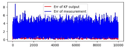
- As another numerical experiment, let’s look at the ROV simulation of 2D trajectories with high measurement noise.
from pylab import *
import numpy as np

def ROVsimulation(procVar,measVar,N,dt):
	#DO NOT CHANGE
	# Function Given for creating simulated data
	acc = zeros((2,N))
	vel = zeros((2,N))
	control_acc = zeros((2,N))
	pos = zeros((2,N))
	meas_pos = zeros((2,N))
	z = zeros((2,N))
	for i in arange(1,N):
		z = normal([0, 0], 0.1)- 0.05*control_acc[:,i-1]
		control_acc[:,i] = control_acc[:,i-1] + z - 0.01*vel[:,i-1]
		vel[:,i] = vel[:,i-1] + control_acc[:,i-1]*dt
		pos[:,i] = pos[:,i-1] + vel[:,i-1]*dt + control_acc[:,i-1]*0.5*dt**2

	acc = normal(control_acc, sqrt(procVar))
	pos = zeros((2,N))
	vel = zeros((2,N))

	for i in arange(1,N):

		vel[:,i] = vel[:,i-1] + acc[:,i-1]*dt
		pos[:,i] = pos[:,i-1] + vel[:,i-1]*dt + acc[:,i-1]*0.5*dt**2


	meas_pos = normal(pos, sqrt(measVar))
	real_pos = pos

	return control_acc, meas_pos, real_pos


def predict(control_acc, dt, procVar , X, P, i):
        F = [[1,dt,0,0], [0,0,0,0], [0,0,1,dt], [0,0,0,0]]
        B = [[0,0],[1,0],[0,0],[0,1]]
        Q = [[procVar,0,0,0],[0,0,0,0],[0,0,procVar,0],[0,0,0,0]]
        X = np.add(np.matmul(F, X), np.matmul(B, control_acc[:,i-1]))
        P = np.add(np.matmul(np.matmul(F, P), np.transpose(F)),Q)
        return X, P

def update( meas_pos, dt, measVar, X, P, i):
        H = [[1,0,0,0],[0,0,1,0]]
        R = [[measVar,0],[0,measVar]]
        K1 = np.matmul(np.matmul(P, np.transpose(H)), np.linalg.inv(np.add(np.matmul(np.matmul(H, P), np.transpose(H)), R)))
        X = np.add(X, np.matmul(K1, np.subtract(meas_pos[:,i], np.matmul(H, X))))
        P = np.subtract(P, np.matmul(np.matmul(K1, H), P))
        return X, P


def your_KalmanFilter(control_acc,meas_pos,procVar,measVar,N,dt):
############################################################################################
#TODO: design kalman filter
#MODEL: position = position + velocity*time_interval + 0.5*acceleration*time_interval**2
#############################################################################################
        approx_pos = zeros((2,N))
        X = [meas_pos[0][0], 1, meas_pos[1][0], 0]
        P = [[0,0,0,0],[0,0,0,0],[0,0,0,0],[0,0,0,0]]
        for i in range(1, len(control_acc[0])):
                X, P = predict(control_acc, dt, procVar, X, P, i)
                X, P = update(meas_pos, dt, measVar, X, P, i)
                approx_pos[0][i] = X[0]
                approx_pos[1][i] = X[2]
        return approx_pos

##############################
#Code starts here
##############################
N = int(1e4)				# number of simulation sample point
dt = 1.0/100.0		# time interval for each sample point
procVar = 0.001		# Process(Prediction) Noise
measVar = 3			# Measurement Noise

[control_acc, meas_pos, real_pos] = ROVsimulation(procVar,measVar,N,dt)
#control_acc: acceleration as a control input signal to the filter
#meas_pos: position measurement
#real_pos: actual position of vehicle(not observable)

approx_pos = your_KalmanFilter(control_acc, meas_pos, procVar, measVar, N, dt)


figure()
plot(approx_pos[0,:],approx_pos[1,:], 'r',label = 'Approx Position')
#plot(meas_pos[0,:],meas_pos[1,:], 'g',label = 'Measured Position')
plot(real_pos[0,:],real_pos[1,:],'b',label = 'True Position')
show()

# Plotting error from real value
figure()
subplot(2,1,1)
plot(norm(approx_pos[:,:]-real_pos[:,:],axis=0), 'r',label = 'Err of KF output')
plot(norm(meas_pos[:,:]-real_pos[:,:],axis=0),'b',label = 'Err of measurement')
legend()
show()
Kalman-based simulation of 2D trajectories: red label is the Approximate Position and blue label is the true trajectory:

Error of KF output (cf. red label above)

True 2D trajectory (blue label) vs noisy measurements (green label)

Error of KF output (red label) vs error of measurements (blue label)
- Let’s examine 2D object tracking using the Extended Kalman Filter (EKF) algorithm
import numpy as np
from math import sin, cos
import matplotlib.pyplot as plt


class KalmanFilter:
    def __init__(self, x, r=np.eye(4), q=np.eye(4)):
        self.x = x
        self.P = np.eye(3)
        self.H = np.eye(3)
        self.Q = q
        self.R = r

        self.state_hist = np.array([self.x.copy()])

    def F(self, v=0., w=0., ang=0.):
        F = np.eye(3)
        F[0, 2] = -(v * sin(ang))
        F[1, 2] = v * cos(ang)
        F[2, 2] = 0.
        return F

    def motion_model(self, prev, ctl):
        x = prev[0]
        y = prev[1]
        thet = prev[2]

        v = ctl[0]
        w = ctl[1]

        x_k1 = x + (v * cos(thet) * DT)
        y_k1 = y + (v * sin(thet) * DT)
        thet_k1 = thet + (w * DT)

        return np.array([x_k1, y_k1, thet_k1])

    def predict(self, controls=np.zeros(2)):
        F = self.F(controls[0], controls[1], self.x[2])
        self.x = self.motion_model(self.x, controls)
        self.P = F @ self.P @ F.T + self.Q

    def update(self, z):
        K2 = np.linalg.inv(self.H @ self.P @ self.H.T + self.R)
        K = self.P @ self.H.T @ K2

        self.x += K @ (z - self.H @ self.x)
        self.P = (np.eye(3) - K @ self.H) @ self.P

        self.state_hist = np.vstack((self.state_hist, self.x))

    def __call__(self, controls, z):
        self.predict(controls)
        self.update(z)


def update(states, controls):
    pos_noise = np.random.normal(0., .1, 2)
    thet_noise = np.random.normal(0., .1, 1)

    states[0] += ((controls[0] * cos(states[2])) * DT) + pos_noise[0]
    states[1] += ((controls[0] * sin(states[2])) * DT) + pos_noise[1]
    states[2] += (controls[1] * DT) + thet_noise[0]


# Must pass a copy of 'states' to this
def sense_state(states):
    pos_noise = np.random.normal(0., .075, 2)
    thet_noise = np.random.normal(0., .075, 1)

    states[0] += pos_noise[0]
    states[1] += pos_noise[1]
    states[2] += thet_noise[0]

    return states


if __name__ == "__main__":
    DT = .1
    #                      x   y  thet
    true_state = np.array([0., .5, 0.])
    true_state_hist = [true_state.copy()]

    cov_est = np.zeros((3, 3))
    cmd = np.array([1.5, 0.35])

    q_mat = np.eye(3) * .1  # Motion Model
    r_mat = np.eye(3) * .025  # Sensor Model
    init_measured_state = sense_state(true_state.copy())
    kf = KalmanFilter(init_measured_state, q_mat, r_mat)
    measured_state_hist = [init_measured_state.copy()]

    err = 0.
    measured_err = 0.

    for i in range(100):
        update(true_state, cmd)
        measured_state = sense_state(true_state.copy())
        kf(cmd, measured_state)
        true_state_hist.append(true_state.copy())
        measured_state_hist.append(measured_state.copy())
        err += np.sum(np.abs(true_state - kf.x))
        measured_err += np.sum(np.abs(true_state - measured_state))

    true_state_hist = np.array(true_state_hist)
    measured_state_hist = np.array(measured_state_hist)

    print("True State: ", [round(ts, 3) for ts in true_state])
    print("KF State: ", [round(xi, 3) for xi in kf.x])
    print("KF Covariance: ")
    print(kf.P)

    print("--------------------------------------")
    print("Kalman Filter Err: ", err)
    print("Measured Err: ", measured_err)

    plt.plot(true_state_hist[:, 0], true_state_hist[:, 1], 'r--', label="True")
    plt.plot(kf.state_hist[:, 0], kf.state_hist[:, 1], 'b--', label="Kalman Filter")
    plt.plot(measured_state_hist[:, 0], measured_state_hist[:, 1], 'gx', label="Measured")
    plt.grid()
    plt.legend()
    plt.xlim(-5., 15.)
    plt.ylim(0., 15.)
    plt.show()

True State:  [-2.606, 7.399, 3.532]
KF State:  [-2.549, 7.388, 3.573]
KF Covariance:
[[ 0.04158589 -0.00592329  0.        ]
 [-0.00592329  0.05317288  0.        ]
 [ 0.          0.          0.02      ]]
--------------------------------------
Kalman Filter Err:  18.349820543394383
Measured Err:  16.900663359808963

3D Analysis
#Basic Imports
import numpy as np
%matplotlib inline
import matplotlib.pyplot as plt
from mpl_toolkits.mplot3d import Axes3D
- Simulated measurement
#Measurement
Hz = 100.0 # Frequency of Vision System
dt = 1.0/Hz
T = 1.0 # s measuremnt time
m = int(T/dt) # number of measurements

px= 0.0 # x Position Start
py= 0.0 # y Position Start
pz= 1.0 # z Position Start

vx = 10.0 # m/s Velocity at the beginning
vy = 0.0 # m/s Velocity
vz = 0.0 # m/s Velocity

c = 0.1 # Drag Resistance Coefficient
d = 0.9 # Damping

Xr=[]
Yr=[]
Zr=[]
for i in range(int(m)):
    accx = -c*vx**2  # Drag Resistance

    vx += accx*dt
    px += vx*dt

    accz = -9.806 + c*vz**2 # Gravitation + Drag
    vz += accz*dt
    pz += vz*dt

    if pz<0.01:
        vz=-vz*d
        pz+=0.02
    if vx<0.1:
        accx=0.0
        accz=0.0

    Xr.append(px)
    Yr.append(py)
    Zr.append(pz)
- Adding random noise
#Add noise
sp= 0.1 # Sigma for position noise

Xm = Xr + sp * (np.random.randn(m))

Ym = Yr + sp * (np.random.randn(m))
Zm = Zr + sp * (np.random.randn(m))
- Plotting the 3D Ball Trajectory observed from Computer Vision System (with Noise)
fig = plt.figure(figsize=(16,9))
ax = fig.add_subplot(111, projection='3d')
ax.scatter(Xm, Ym, Zm, c='gray')
ax.set_xlabel('X')
ax.set_ylabel('Y')
ax.set_zlabel('Z')
plt.title('Ball Trajectory observed from Computer Vision System (with Noise)')
# Axis equal
max_range = np.array([Xm.max()-Xm.min(), Ym.max()-Ym.min(), Zm.max()-Zm.min()]).max() / 3.0
mean_x = Xm.mean()
mean_y = Ym.mean()
mean_z = Zm.mean()
ax.set_xlim(mean_x - max_range, mean_x + max_range)
ax.set_ylim(mean_y - max_range, mean_y + max_range)
ax.set_zlim(mean_z - max_range, mean_z + max_range)

- Implementing the opencv KF
#cv2 kalman
import cv2
v = dt
a = 0.5 * (dt**2)
kalman = cv2.KalmanFilter(9, 3, 0)

kalman.measurementMatrix = np.array([
        [1, 0, 0, v, 0, 0, a, 0, 0],
        [0, 1, 0, 0, v, 0, 0, a, 0],
        [0, 0, 1, 0, 0, v, 0, 0, a]
    ],np.float32)

kalman.transitionMatrix = np.array([
        [1, 0, 0, v, 0, 0, a, 0, 0],
        [0, 1, 0, 0, v, 0, 0, a, 0],
        [0, 0, 1, 0, 0, v, 0, 0, a],
        [0, 0, 0, 1, 0, 0, v, 0, 0],
        [0, 0, 0, 0, 1, 0, 0, v, 0],
        [0, 0, 0, 0, 0, 1, 0, 0, v],
        [0, 0, 0, 0, 0, 0, 1, 0, 0],
        [0, 0, 0, 0, 0, 0, 0, 1, 0],
        [0, 0, 0, 0, 0, 0, 0, 0, 1]
    ],np.float32)

kalman.processNoiseCov = np.array([
        [1, 0, 0, 0, 0, 0, 0, 0, 0],
        [0, 1, 0, 0, 0, 0, 0, 0, 0],
        [0, 0, 1, 0, 0, 0, 0, 0, 0],
        [0, 0, 0, 1, 0, 0, 0, 0, 0],
        [0, 0, 0, 0, 1, 0, 0, 0, 0],
        [0, 0, 0, 0, 0, 1, 0, 0, 0],
        [0, 0, 0, 0, 0, 0, 1, 0, 0],
        [0, 0, 0, 0, 0, 0, 0, 1, 0],
        [0, 0, 0, 0, 0, 0, 0, 0, 1]
    ],np.float32) * 0.007

kalman.measurementNoiseCov = np.array([
        [1, 0, 0],
        [0, 1, 0],
        [0, 0 ,1]
    ],np.float32) * sp

kalman.statePre = np.array([
                                [np.float32(Xm[0])], [np.float32(Ym[0])], [np.float32(Zm[0])]
                               , [np.float32(0.)], [np.float32(0.)], [np.float32(0.)]
                               , [np.float32(0.)], [np.float32(0.)], [np.float32(0.)]
                           ])
- Calculating the 3D trajectories
mp = np.array((3, 1), np.float32) # measurement
tp = np.zeros((3, 1), np.float32)
xt = []
yt = []
zt = []
for i in range(m):
    mp = np.array([
        [np.float32(Xm[i])],
        [np.float32(Ym[i])],
        [np.float32(Zm[i])]
    ])
    kalman.correct(mp)
    tp = kalman.predict()
    xt.append(float(tp[0]))
    yt.append(float(tp[1]))
    zt.append(float(tp[2]))
- Plotting the 3D Ball Trajectory estimated with KF
fig = plt.figure(figsize=(16,9))
ax = fig.add_subplot(111, projection='3d')
ax.plot(xt,yt,zt, label='Kalman Filter Estimate', c='green')
ax.plot(Xr, Yr, Zr, c='red', label='Real')
ax.scatter(Xm, Ym, Zm, c='blue', label='Noise')
ax.set_xlabel('X')
ax.set_ylabel('Y')
ax.set_zlabel('Z')
ax.legend()
plt.title('Ball Trajectory estimated with Kalman Filter')

# Axis equal
max_range = np.array([Xm.max()-Xm.min(), Ym.max()-Ym.min(), Zm.max()-Zm.min()]).max() / 3.0
mean_x = Xm.mean()
mean_y = Ym.mean()
mean_z = Zm.mean()
ax.set_xlim(mean_x - max_range, mean_x + max_range)
ax.set_ylim(mean_y - max_range, mean_y + max_range)
ax.set_zlim(mean_z - max_range, mean_z + max_range)

- We can see that opencv offers a robust Kalman filter approach for accurately estimating the 3D position of a moving object.
Summary
- This paper performs the noise sensitivity analysis of standard and extended state-of-the-art Kalman filters (KF) used for object tracking in real time.
- We examined different configurations of KF by executing a series of 1D, 2D and 3D numerical simulations.
- We analyzed the influence of varying noise parameters and the choice of time discrete model onto accuracy of object position and speed estimation.
- All KF methods come with realistic accuracy statements, and are compared on a few challenging target tracking examples.
- Results have shown that the KF is optimal for the considered problem. However, it uses more information than any of the other algorithms, and knows which measurements can be trusted and which are bad. The knowledge about process and measurement noise is complementary and yields highly confident estimation results.
- Key assumption: the KF algorithm was derived under the premises that the process noise is well behaved, and indeed it works very well if outliers only appear in the measurement noise. The accuracy can be significantly improved by increasing and/or updating the utilized process noise covariance.
- Bottom line: our numerical experiments using Python have confirmed that the performance of the KF algorithms is appropriate for estimating moving object position and speed in real time.
- Business value: KF object tracking has many practical applications such as automated surveillance system, military guidance, traffic management system, fault detection system, AI and robot vision systems.
- The road ahead: our next steps will involve Kalman-based multiple objects tracking algorithms combined with studies of correlated noise in KF.
Explore More
- Anatomy of the Robust 1D Kalman Filter
- Kalman-Based Target Trajectory Tracking Performance QC Analysis
- Sensitivity of Kalman Object Tracking to Noise & State Errors


One-Time
Monthly
Yearly
Make a one-time donation
Make a monthly donation
Make a yearly donation
Choose an amount
€5.00
€15.00
€100.00
€5.00
€15.00
€100.00
€5.00
€15.00
€100.00
Or enter a custom amount
€
Your contribution is appreciated.
Your contribution is appreciated.
Your contribution is appreciated.
DonateDonate monthlyDonate yearly
Leave a comment