
Featured Image via Canva.
- MLflow is a modern MLOps tool for data project collaboration.
- In this post, we’ll walk through a few simplified MLflow projects that let you package data science code in a reproducible and reusable way.
- MLflow, at its core, provides a suite of tools aimed at simplifying the ML workflow. It is tailored to assist ML practitioners throughout the various stages of ML development and deployment.
Table of Contents
- Local Environment Setup
- ElasticNet Model Optimization
- Model SHAP Explanations
- Sentence Transformers
- Summary
- Explore More
Local Environment Setup
- You install MLflow by running pip:
!pip install mlflow
- Setting the working directory YOURPATH
import os
os.chdir('YOURPATH')    # Set working directory
os. getcwd()
- It is recommended to create a new python environment for MLflow using Anaconda.
- You can run existing projects with the
mlflow runcommand, which runs a project from our local directory. - To use certain MLflow modules and functionality, you may need to install extra libraries. For example, the
mlflow.tensorflowmodule requires TensorFlow to be installed. - We avoid running directly from a clone of MLflow as doing so would cause our tests to use MLflow from source, rather than our PyPi installation of MLflow.
- Read more here.
ElasticNet Model Optimization
- Let’s look at the
train.pynbJupyter notebook predicts the quality of wine using sklearn.linear_model.ElasticNet.
# Wine Quality Sample
def train(in_alpha, in_l1_ratio):
    import logging
    import warnings

    import numpy as np
    import pandas as pd
    from sklearn.linear_model import ElasticNet
    from sklearn.metrics import mean_absolute_error, mean_squared_error, r2_score
    from sklearn.model_selection import train_test_split

    import mlflow
    import mlflow.sklearn
    from mlflow.models import infer_signature

    logging.basicConfig(level=logging.WARN)
    logger = logging.getLogger(__name__)

    def eval_metrics(actual, pred):
        rmse = np.sqrt(mean_squared_error(actual, pred))
        mae = mean_absolute_error(actual, pred)
        r2 = r2_score(actual, pred)
        return rmse, mae, r2

    warnings.filterwarnings("ignore")
    np.random.seed(40)

    # Read the wine-quality csv file from the URL
    csv_url = (
        "http://archive.ics.uci.edu/ml/machine-learning-databases/wine-quality/winequality-red.csv"
    )
    try:
        data = pd.read_csv(csv_url, sep=";")
    except Exception as e:
        logger.exception(
            "Unable to download training & test CSV, check your internet connection. Error: %s", e
        )

    # Split the data into training and test sets. (0.75, 0.25) split.
    train, test = train_test_split(data)

    # The predicted column is "quality" which is a scalar from [3, 9]
    train_x = train.drop(["quality"], axis=1)
    test_x = test.drop(["quality"], axis=1)
    train_y = train[["quality"]]
    test_y = test[["quality"]]

    # Set default values if no alpha is provided
    alpha = 0.5 if float(in_alpha) is None else float(in_alpha)

    # Set default values if no l1_ratio is provided
    l1_ratio = 0.5 if float(in_l1_ratio) is None else float(in_l1_ratio)

    # Useful for multiple runs (only doing one run in this sample notebook)
    with mlflow.start_run():
        # Execute ElasticNet
        lr = ElasticNet(alpha=alpha, l1_ratio=l1_ratio, random_state=42)
        lr.fit(train_x, train_y)

        # Evaluate Metrics
        predicted_qualities = lr.predict(test_x)
        (rmse, mae, r2) = eval_metrics(test_y, predicted_qualities)

        # Print out metrics
        print(f"Elasticnet model (alpha={alpha:f}, l1_ratio={l1_ratio:f}):")
        print("  RMSE: %s" % rmse)
        print("  MAE: %s" % mae)
        print("  R2: %s" % r2)

        # Infer model signature
        predictions = lr.predict(train_x)
        signature = infer_signature(train_x, predictions)

        # Log parameter, metrics, and model to MLflow
        mlflow.log_param("alpha", alpha)
        mlflow.log_param("l1_ratio", l1_ratio)
        mlflow.log_metric("rmse", rmse)
        mlflow.log_metric("r2", r2)
        mlflow.log_metric("mae", mae)

        mlflow.sklearn.log_model(lr, "model", signature=signature)
- Output of the linear regression with combined L1 and L2 priors as regularizer:
train(0.5, 0.5)
Elasticnet model (alpha=0.500000, l1_ratio=0.500000):
  RMSE: 0.793164022927685
  MAE: 0.6271946374319586
  R2: 0.10862644997792625
train(0.2, 0.2)
Elasticnet model (alpha=0.200000, l1_ratio=0.200000):
  RMSE: 0.7336400911821402
  MAE: 0.5643841279275427
  R2: 0.2373946606358417
train(0.1, 0.1)
Elasticnet model (alpha=0.100000, l1_ratio=0.100000):
  RMSE: 0.7128829045893679
  MAE: 0.5462202174984664
  R2: 0.2799376066653345
- The optimal values of alpha and l1_ratio can be determined by minimizing RMSE or MAE within the 2D grid search loop.
Model SHAP Explanations
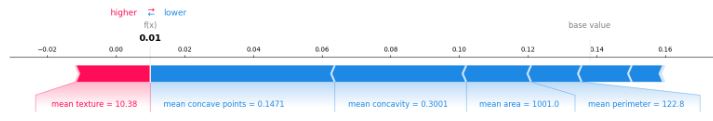
- Example 1: Breast Cancer SHAP explainer
import os

import numpy as np
import shap
from sklearn.datasets import load_breast_cancer
from sklearn.ensemble import RandomForestClassifier

import mlflow
from mlflow.artifacts import download_artifacts
from mlflow.tracking import MlflowClient

# prepare training data
X, y = load_breast_cancer(return_X_y=True, as_frame=True)
X = X.iloc[:50, :8]
y = y.iloc[:50]

# train a model
model = RandomForestClassifier()
model.fit(X, y)

# log an explanation
with mlflow.start_run() as run:
    mlflow.shap.log_explanation(lambda X: model.predict_proba(X)[:, 1], X)

# list artifacts
client = MlflowClient()
artifact_path = "model_explanations_shap"
artifacts = [x.path for x in client.list_artifacts(run.info.run_id, artifact_path)]
print("# artifacts:")
print(artifacts)

# load back the logged explanation
dst_path = download_artifacts(run_id=run.info.run_id, artifact_path=artifact_path)
base_values = np.load(os.path.join(dst_path, "base_values.npy"))
shap_values = np.load(os.path.join(dst_path, "shap_values.npy"))

# show a force plot
shap.force_plot(float(base_values), shap_values[0, :], X.iloc[0, :], matplotlib=True)
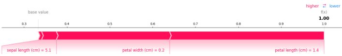
- Example 2: Iris Classification SHAP explainer
import numpy as np
import shap
from sklearn.datasets import load_iris
from sklearn.ensemble import RandomForestClassifier

import mlflow
from mlflow.artifacts import download_artifacts
from mlflow.tracking import MlflowClient

# prepare training data
X, y = load_iris(return_X_y=True, as_frame=True)


# train a model
model = RandomForestClassifier()
model.fit(X, y)

# log an explanation
with mlflow.start_run() as run:
    mlflow.shap.log_explanation(model.predict_proba, X)

# list artifacts
client = MlflowClient()
artifact_path = "model_explanations_shap"
artifacts = [x.path for x in client.list_artifacts(run.info.run_id, artifact_path)]
print("# artifacts:")
print(artifacts)

# load back the logged explanation
dst_path = download_artifacts(run_id=run.info.run_id, artifact_path=artifact_path)
base_values = np.load(os.path.join(dst_path, "base_values.npy"))
shap_values = np.load(os.path.join(dst_path, "shap_values.npy"))

# show a force plot
shap.force_plot(base_values[0], shap_values[0, 0, :], X.iloc[0, :], matplotlib=True)
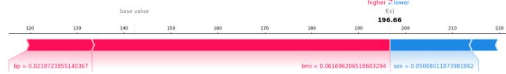
- Example 3: Diabetes-2 SHAP explainer
import numpy as np
import shap
from sklearn.datasets import load_diabetes
from sklearn.linear_model import LinearRegression

import mlflow
from mlflow.artifacts import download_artifacts
from mlflow.tracking import MlflowClient

# prepare training data
X, y = load_diabetes(return_X_y=True, as_frame=True)
X = X.iloc[:50, :4]
y = y.iloc[:50]

# train a model
model = LinearRegression()
model.fit(X, y)

# log an explanation
with mlflow.start_run() as run:
    mlflow.shap.log_explanation(model.predict, X)

# list artifacts
client = MlflowClient()
artifact_path = "model_explanations_shap"
artifacts = [x.path for x in client.list_artifacts(run.info.run_id, artifact_path)]
print("# artifacts:")
print(artifacts)

# load back the logged explanation
dst_path = download_artifacts(run_id=run.info.run_id, artifact_path=artifact_path)
base_values = np.load(os.path.join(dst_path, "base_values.npy"))
shap_values = np.load(os.path.join(dst_path, "shap_values.npy"))

# show a force plot
shap.force_plot(float(base_values), shap_values[0, :], X.iloc[0, :], matplotlib=True)
Sentence Transformers
- Consider MLflow Sentence-Transformers Flavor
- Example 1: MLflow chatbot using microsoft/DialoGPT-medium
import transformers

import mlflow

conversational_pipeline = transformers.pipeline(model="microsoft/DialoGPT-medium")

signature = mlflow.models.infer_signature(
    "Hi there, chatbot!",
    mlflow.transformers.generate_signature_output(conversational_pipeline, "Hi there, chatbot!"),
)

with mlflow.start_run():
    model_info = mlflow.transformers.log_model(
        transformers_model=conversational_pipeline,
        artifact_path="chatbot",
        task="conversational",
        signature=signature,
        input_example="A clever and witty question",
    )

# Load the conversational pipeline as an interactive chatbot

chatbot = mlflow.pyfunc.load_model(model_uri=model_info.model_uri)

first = chatbot.predict("What is the best way to get to Antarctica?")

print(f"Response: {first}")

second = chatbot.predict("What kind of boat should I use?")

print(f"Response: {second}")
Response: I think you can get there by boat.
Response: A boat that can go to Antarctica.
- Example 2: Translation with Transformers and MLflow
import transformers

import mlflow

translation_pipeline = transformers.pipeline(
    task="translation_en_to_fr",
    model=transformers.T5ForConditionalGeneration.from_pretrained("t5-small"),
    tokenizer=transformers.T5TokenizerFast.from_pretrained("t5-small", model_max_length=100),
)

signature = mlflow.models.infer_signature(
    "Hi there, chatbot!",
    mlflow.transformers.generate_signature_output(translation_pipeline, "Hi there, chatbot!"),
)

with mlflow.start_run():
    model_info = mlflow.transformers.log_model(
        transformers_model=translation_pipeline,
        artifact_path="french_translator",
        signature=signature,
    )

translation_components = mlflow.transformers.load_model(
    model_info.model_uri, return_type="components"
)

for key, value in translation_components.items():
    print(f"{key} -> {type(value).__name__}")

response = translation_pipeline("MLflow is great!")

print(response)

reconstructed_pipeline = transformers.pipeline(**translation_components)

reconstructed_response = reconstructed_pipeline(
    "transformers makes using Deep Learning models easy and fun!"
)

print(reconstructed_response)
task -> str
device_map -> str
model -> T5ForConditionalGeneration
tokenizer -> T5TokenizerFast
framework -> str
[{'translation_text': 'MLflow est formidable!'}]
[{'translation_text': "Les transformateurs rendent l'utilisation de modèles Deep Learning facile et amusante!"}]
Summary
- We have explored the concepts of MLflow hyperparameter tuning by predicting the quality of wine using sklearn.linear_model.ElasticNet.
- We have looked at mlflow.shap using the breast cancer, diabetes and iris datasets. SHAP values are based on game theory and assign an importance value to each feature in a model. Features with positive SHAP values positively impact the prediction, while those with negative values have a negative impact. The magnitude is a measure of how strong the effect is.
- The chatbot VA and translation examples have demonstrated that the MLflow Sentence Transformers provide a powerful interface for managing transformer models and pipelines from libraries like Hugging Face’s Transformers.
Explore More
- MLflow examples
- Hugging Face NLP, Streamlit/Dash & Jupyter PyGWalker EDA, TensorFlow Keras & Gradio App Deployment Showcase


One-Time
Monthly
Yearly
Make a one-time donation
Make a monthly donation
Make a yearly donation
Choose an amount
€5.00
€15.00
€100.00
€5.00
€15.00
€100.00
€5.00
€15.00
€100.00
Or enter a custom amount
€
Your contribution is appreciated.
Your contribution is appreciated.
Your contribution is appreciated.

Leave a comment