H2O AutoML Malware Detection

Malware detection is a crucial aspect of cybersecurity.
The objective of this study is to perform effective AI-powered malware detection and interpretation with the open-source H2O AutoML algorithm.
H2O’s AutoML can be used for automating the Machine Learning (ML) workflow, which includes automatic training and tuning of many models within a user-specified time-limit. AutoML automates most of the steps in an ML pipeline, with a minimum amount of human effort and without compromising on its performance.
The input Kaggle dataset is a result of a R&D about ML & Malware Detection. It was built using a Python Library and contains benign and malicious data from PE Files.

Table of Contents

Model Training
Model Optimization
Classification Report
Model Interpretations
Summary
Explore More

Model Training

Setting the working directory YOURPATH

import os
os.chdir('YOURPATH')    # Set working directory
os. getcwd()

Importing key libraries, reading the data and defining the H2O AutoML framework

import numpy as np
import pandas as pd 
import pickle
import seaborn as sns
import matplotlib.pyplot as plt
from sklearn.metrics import confusion_matrix, classification_report, accuracy_score

import h2o
from h2o.automl import H2OAutoML
h2o.init(max_mem_size='2G')
data = pd.read_csv('dataset_malwares.csv')
from h2o.frame import H2OFrame
data = H2OFrame(data)

Splitting the data and training the model

train, test = data.split_frame(ratios=[0.6], seed=42)
from h2o.automl import H2OAutoML

automl = H2OAutoML(max_runtime_secs=600)  # Set the maximum runtime in seconds
automl.train(x=data.columns[:-1], y='Malware', training_frame = train)

Output logs:

AutoML: XGBoost is not available; skipping it.
Model Details
=============
H2OStackedEnsembleEstimator : Stacked Ensemble
Model Key: StackedEnsemble_AllModels_3_AutoML_2_20240211_162431
Model Summary for Stacked Ensemble:
key	value
Stacking strategy	cross_validation
Number of base models (used / total)	7/49
# GBM base models (used / total)	6/43
# DRF base models (used / total)	0/2
# GLM base models (used / total)	0/1
# DeepLearning base models (used / total)	1/3
Metalearner algorithm	GLM
Metalearner fold assignment scheme	Random
Metalearner nfolds	5
Metalearner fold_column	None
Custom metalearner hyperparameters	None
ModelMetricsRegressionGLM: stackedensemble
** Reported on train data. **

MSE: 0.0009636378361646813
RMSE: 0.031042516588779996
MAE: 0.008877334165576591
RMSLE: 0.02408848192111684
Mean Residual Deviance: 0.0009636378361646813
R^2: 0.9949665112607115
Null degrees of freedom: 9975
Residual degrees of freedom: 9968
Null deviance: 1909.8904021504356
Residual deviance: 9.61325105357886
AIC: -40952.613530641036
ModelMetricsRegressionGLM: stackedensemble
** Reported on cross-validation data. **

MSE: 0.00671905903384776
RMSE: 0.08196986662089771
MAE: 0.021946099162326017
RMSLE: 0.0578426755882866
Mean Residual Deviance: 0.00671905903384776
R^2: 0.9647434373633934
Null degrees of freedom: 11797
Residual degrees of freedom: 11791
Null deviance: 2249.4329600946585
Residual deviance: 79.27145848133587
AIC: -25525.84523210719
Cross-Validation Metrics Summary:
mean	sd	cv_1_valid	cv_2_valid	cv_3_valid	cv_4_valid	cv_5_valid
mae	0.0219382	0.0009372	0.0213027	0.0215373	0.0217661	0.0235886	0.0214964
mean_residual_deviance	0.0067135	0.0006209	0.0062748	0.006535	0.0069114	0.0076946	0.0061516
mse	0.0067135	0.0006209	0.0062748	0.006535	0.0069114	0.0076946	0.0061516
null_deviance	449.8866	16.695866	457.94696	466.87103	435.76636	460.2754	428.57324
r2	0.9647123	0.0034319	0.9682267	0.966678	0.9624521	0.9598925	0.9663121
residual_deviance	15.854292	1.6567098	14.526201	15.54023	16.33865	18.459446	14.406931
rmse	0.0818678	0.0037333	0.0792137	0.0808394	0.0831351	0.0877191	0.0784318
rmsle	0.0577558	0.0029666	0.0563536	0.0575922	0.0583191	0.0622814	0.0542329

Performing test predictions of the automl leader

predictions = automl.leader.predict(test)

Model Optimization

Selecting the best model from the leaderboard in terms of the ML evaluation metrics

from sklearn.metrics import precision_score, recall_score, f1_score

# Define evaluation metrics
def evaluate_model(true_labels, predicted_labels):
    precision = precision_score(true_labels, predicted_labels)
    recall = recall_score(true_labels, predicted_labels)
    f1 = f1_score(true_labels, predicted_labels)
    return precision, recall, f1

# List of models from the leaderboard
models = automl.leaderboard['model_id'].as_data_frame()['model_id'].tolist()

# Initialize best model
best_model = None
best_metrics = {'precision': 0, 'recall': 0, 'f1': 0}

# Evaluate each model and select the best one
for model_id in models:
    # Make predictions
    predictions = automl.leader.predict(test)
    predicted_probabilities = predictions['predict'].as_data_frame()['predict'].values
    predicted_labels = (predicted_probabilities > 0.5).astype(int)
    
    # Evaluate the model
    precision, recall, f1 = evaluate_model(true_labels, predicted_labels)
    
    # Update best model if current model is better
    if f1 > best_metrics['f1']:
        best_model = model_id
        best_metrics = {'precision': precision, 'recall': recall, 'f1': f1}

# Print information about the best model
print(f"Best Model: {best_model}")
print("Best Model Metrics:")
print(f"Precision: {best_metrics['precision']:.4f}")
print(f"Recall: {best_metrics['recall']:.4f}")
print(f"F1 Score: {best_metrics['f1']:.4f}")

Output

Best Model: StackedEnsemble_AllModels_3_AutoML_2_20240211_162431
Best Model Metrics:
Precision: 0.9933
Recall: 0.9983
F1 Score: 0.9958

Plotting the Pareto Front for H2O AutoML

pf = automl.pareto_front()
pf.figure()
pf
model_id	rmse	mse	mae	rmsle	mean_residual_deviance	training_time_ms	predict_time_per_row_ms	algo
StackedEnsemble_AllModels_3_AutoML_2_20240211_162431	0.0819699	0.00671906	0.0219461	0.0578427	0.00671906	510	0.151789	StackedEnsemble
StackedEnsemble_BestOfFamily_4_AutoML_2_20240211_162431	0.0842577	0.00709936	0.0224664	0.0593384	0.00709936	365	0.019229	StackedEnsemble
GBM_grid_1_AutoML_2_20240211_162431_model_29	0.0842626	0.00710019	0.0218079	0.0593146	0.00710019	3638	0.015837	GBM
GBM_grid_1_AutoML_2_20240211_162431_model_13	0.085033	0.00723061	0.0214841	0.0595172	0.00723061	1543	0.013421	GBM
GBM_grid_1_AutoML_2_20240211_162431_model_28	0.0859028	0.00737929	0.023693	0.0598147	0.00737929	1270	0.011117	GBM
GBM_grid_1_AutoML_2_20240211_162431_model_1	0.0872463	0.00761192	0.0176017	0.0605518	0.00761192	1716	0.009195	GBM
XRT_1_AutoML_2_20240211_162431	0.0988725	0.00977577	0.0295303	0.069559	0.00977577	972	0.006904	DRF
DRF_1_AutoML_2_20240211_162431	0.100821	0.0101649	0.02576	0.0709873	0.0101649	714	0.006876	DRF
GBM_grid_1_AutoML_2_20240211_162431_model_38	0.136559	0.0186483	0.0834828	0.101459	0.0186483	121	0.001727	GBM
GLM_1_AutoML_2_20240211_162431	0.253971	0.0645013	0.169792	nan	0.0645013	34	0.001054	GLM

Classification Report

Extracting predicted probabilities and calculating the test accuracy

# Extract predicted probabilities
predicted_probabilities = predictions['predict'].as_data_frame()['predict'].values

# Convert predicted probabilities to class labels
predicted_labels = (predicted_probabilities > 0.5).astype(int)

# Ensure true_labels is of the same type (H2OFrame to Pandas DataFrame)
true_labels = test['Malware'].as_data_frame()['Malware'].values

# Calculate accuracy
accuracy = accuracy_score(true_labels, predicted_labels)

print(f'Test Accuracy: {accuracy * 100:.2f}%')
Test Accuracy: 99.37%

Generating the ML classification report

# Confusion Matrix
cm = confusion_matrix(true_labels, predicted_labels)
print("Confusion Matrix:")
print(cm)

# Classification Report
report = classification_report(true_labels, predicted_labels)
print("Classification Report:")
print(report)

Confusion Matrix:
[[1950   39]
 [  10 5814]]
Classification Report:
              precision    recall  f1-score   support

           0       0.99      0.98      0.99      1989
           1       0.99      1.00      1.00      5824

    accuracy                           0.99      7813
   macro avg       0.99      0.99      0.99      7813
weighted avg       0.99      0.99      0.99      7813

Plotting the confusion matrix

# Assuming 'true_labels' and 'predicted_labels' are your true and predicted labels
cm = confusion_matrix(true_labels, predicted_labels)

# Plotting the Confusion Matrix
plt.figure(figsize=(7, 5))
sns.heatmap(cm, annot=True, fmt="d", cmap="Blues", xticklabels=['Non-Malware', 'Malware'], yticklabels=['Non-Malware', 'Malware'])
plt.title('Confusion Matrix')
plt.xlabel('Predicted Label')
plt.ylabel('True Label')
plt.show()

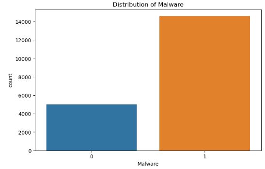
Converting H2OFrame to Pandas DataFrame and plotting the Distribution of Malware

# Convert H2OFrame to Pandas DataFrame
data_pd = data.as_data_frame()

plt.figure(figsize=(8, 5))
sns.countplot(x='Malware', data=data_pd)
plt.title('Distribution of Malware')
plt.show()

Plotting ROC and Precision-Recall Curves

from sklearn.metrics import roc_curve, precision_recall_curve, auc

# Assuming you have true_labels and predicted_probabilities
fpr, tpr, _ = roc_curve(true_labels, predicted_probabilities)
precision, recall, _ = precision_recall_curve(true_labels, predicted_probabilities)

plt.figure(figsize=(10, 5))

# ROC Curve
plt.subplot(1, 2, 1)
plt.plot(fpr, tpr, color='darkorange', lw=2, label='ROC curve (AUC = {:.2f})'.format(auc(fpr, tpr)))
plt.plot([0, 1], [0, 1], color='navy', lw=2, linestyle='--')
plt.xlabel('False Positive Rate')
plt.ylabel('True Positive Rate')
plt.title('Receiver Operating Characteristic (ROC) Curve')
plt.legend()

# Precision-Recall Curve
plt.subplot(1, 2, 2)
plt.plot(recall, precision, color='blue', lw=2, label='Precision-Recall curve')
plt.xlabel('Recall')
plt.ylabel('Precision')
plt.title('Precision-Recall Curve')
plt.legend()

plt.tight_layout()
plt.show()

Model Interpretations

Leaderboard shows models with their metrics and their predictions for a given row. When provided with H2O AutoML object, the leaderboard shows 5-fold cross-validated metrics by default (depending on the H2O AutoML settings), otherwise it shows metrics computed on the frame. At most 20 models are shown by default.

model_id	rmse	mse	mae	rmsle	mean_residual_deviance	training_time_ms	predict_time_per_row_ms	algo	predict
StackedEnsemble_AllModels_3_AutoML_2_20240211_162431	0.0773485	0.0059828	0.0200016	0.0530366	0.0059828	510	0.030086	StackedEnsemble	1.00686
GBM_grid_1_AutoML_2_20240211_162431_model_29	0.0783545	0.00613944	0.0192429	0.0535055	0.00613944	3638	0.016226	GBM	1.00446
StackedEnsemble_BestOfFamily_4_AutoML_2_20240211_162431	0.0784865	0.00616014	0.0198713	0.053641	0.00616014	365	0.016358	StackedEnsemble	1.00637
GBM_grid_1_AutoML_2_20240211_162431_model_13	0.0787041	0.00619433	0.0188041	0.05397	0.00619433	1543	0.012054	GBM	1.0046
StackedEnsemble_AllModels_2_AutoML_2_20240211_162431	0.0792631	0.00628264	0.0201192	0.0549249	0.00628264	592	0.04274	StackedEnsemble	1.00668
StackedEnsemble_AllModels_1_AutoML_2_20240211_162431	0.080609	0.00649781	0.0213402	0.0557984	0.00649781	613	0.049477	StackedEnsemble	1.00718
StackedEnsemble_BestOfFamily_3_AutoML_2_20240211_162431	0.0807443	0.00651964	0.0209621	0.0559776	0.00651964	298	0.014538	StackedEnsemble	1.00649
GBM_grid_1_AutoML_2_20240211_162431_model_16	0.0809532	0.00655342	0.0215635	0.0557101	0.00655342	4199	0.017187	GBM	1.00496
GBM_grid_1_AutoML_2_20240211_162431_model_19	0.0810464	0.00656851	0.0225983	0.0560315	0.00656851	1136	0.017246	GBM	1.00152
GBM_grid_1_AutoML_2_20240211_162431_model_35	0.0810495	0.00656902	0.0210852	0.0561155	0.00656902	990	0.014264	GBM	1.00752
[20 rows x 10 columns]

SHAP explanation shows contribution of features for a given instance. The sum of the feature contributions and the bias term is equal to the raw prediction of the model, i.e., prediction before applying inverse link function. H2O implements TreeSHAP which when the features are correlated, can increase contribution of a feature that had no influence on the prediction.

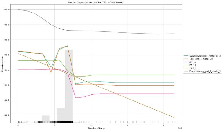
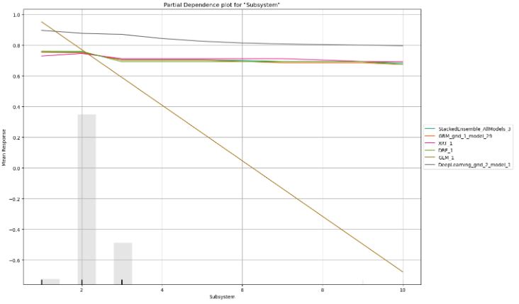
Partial dependence plot (PDP) gives a graphical depiction of the marginal effect of a variable on the response. The effect of a variable is measured in change in the mean response. PDP assumes independence between the feature for which is the PDP computed and the rest.

Partial dependence plot for column=’MajorLinkerVersion’

column='MajorLinkerVersion'
pd_plot = automl.pd_multi_plot(test, column)

Partial dependence plot for column='MajorLinkerVersion'

Partial dependence plot for column=’TimeDateStamp’

column='TimeDateStamp'
pd_plot = automl.pd_multi_plot(test, column)

Partial dependence plot for column='TimeDateStamp'

Partial dependence plot for column=’Subsystem’

column='Subsystem'
pd_plot = automl.pd_multi_plot(test, column)

Partial dependence plot for column='Subsystem'

Summary

Cyberattacks are currently the leading cause of concern in the tech world.
The present proof-of-concept study is dedicated to evaluation and potential integration of ML algorithms to identify malware effectively and rapidly.

Our validation tests confirm that the H2O AutoML workflow can accurately classify whether a given PE file is malware or not.
We have used 7 GBM base models and 1 Deep Learning base model.
Output Model Details: H2OStackedEnsembleEstimator or Stacked Ensemble (SE).
Optimized SE model metrics are as follows:
Precision: 0.9933
Recall: 0.9983
F1 Score: 0.9958
SHAP explanation has shown contributions of features for a given instance.
We have compared partial dependence plots for the top 3 features such as MajorLinkerVersion, TimeDateStamp, and Subsystem.
This evaluation project supports related R&D products and solutions such as H2O’s AI and information security, Automatic Fraud Detection, and Auto_Malware_detection_with_h2o.

Explore More

Go back

Your message has been sent

Make a one-time donation

Make a monthly donation

Make a yearly donation

Choose an amount

€5.00

€15.00

€100.00

€5.00

€15.00

€100.00

€5.00

€15.00

€100.00

Or enter a custom amount

€

Your contribution is appreciated.

Donate Donate monthly Donate yearly

H2O AutoML Malware Detection

Model Training

Model Optimization

Classification Report

Model Interpretations

Summary

Explore More

Your message has been sent

Make a one-time donation

Make a monthly donation

Make a yearly donation

Discover more from Our Blogs

2 responses to “H2O AutoML Malware Detection”

Leave a reply to H2O AutoML Malware Detection F1 0.99 by Optimizing 8 ML Models with SHAP XAI | by Alexzap | Jul, 2024 – Artificial Intelligence Article Cancel reply

H2O AutoML Malware Detection

Model Training

Model Optimization

Classification Report

Model Interpretations

Summary

Explore More

Your message has been sent

Make a one-time donation

Make a monthly donation

Make a yearly donation

Share this:

Discover more from Our Blogs

2 responses to “H2O AutoML Malware Detection”

Leave a reply to H2O AutoML Malware Detection F1 0.99 by Optimizing 8 ML Models with SHAP XAI | by Alexzap | Jul, 2024 – Artificial Intelligence Article Cancel reply

Discover more from Our Blogs