Photo by Kelly on Pexels.
- Based upon the previous study, we continue evaluating performance of the Kalman Filter (KF) by walking through some numerical tests.
- In the presence of uncertainty, one of the most difficult issues for tracking in control systems is to estimate the accuracy and precision of hidden variables.
- KF is considered as the widely adapted estimation algorithm for object tracking applications.
- KF is an optimal estimation algorithm used to estimate states of a dynamic system from uncertain measurements. It takes measurements over time and creates a prediction of the next measurements.
- In this post, we will see a practical approach on how to use KF to track and predict the trajectory of an object.
- Our objective is to track the trajectory of a target by using the basics of KF and compare the filter output and the original trajectory.
Table of Contents
- The Kalman Filter Intuition
- Formulation of a Problem
- Linear Position-Time Path
- Parabolic Position-Time Path
- Extended Kalman Filter (EKF)
- Tracking the Bike’s Path
- Unscented Kalman Filter (UKF)
- Industry Application in Dynamic Positioning System
- Smoothed Position and Speed Estimates
- Radar EKF Trajectory
- Conclusions
- Explore More
- References
The Kalman Filter Intuition
- KF is used for object tracking when you have estimates of object position, measured with error.
- If you are tracking only in 2-D and want to estimate position in 3-D, the third dimension is another state variable you do not measure directly.
- Main idea of KF: we want to estimate the next object position incorporating only the three parameters: object motion model; measurement noise; process noise.
- The KF cycle: First the filter predicts the next state from the provided state transition, then the noisy measurement information is incorporated in the correction phase. The cycle is repeated.
- The actual KF algorithm is implemented as follows:
- Measurement #1 initializes system state estimate & error covariance
- Measurement #2 re-initializes system state estimate & error covariance
- Measurement #3 predicts system state estimate & error covariance to measurement time
- Compute the Kalman gain
- Estimate the system state & error covariance at the measurement time, go to step 3.
- Read more about KF here.
Formulation of a Problem
- Despite the large number of investigations into Kalman filter trackers, the optimal selection of a process noise model has not been discussed.
- Although various criteria have been proposed and investigated for the design of Kalman filters and its variants to achieve better tracking accuracy, robustness, and real-time capability, relationship between these performance indices and the model parameters such as the process noise variance is not discussed even in recent studies.
- Another significant problem in a measurement model of the conventional Kalman tracking filter is that most studies consider only position measurements and therefore cannot make full use of modern sensors that are able to measure velocity, such as ultrawideband Doppler radar. Moreover, sensor fusion based on IoT also enables the simultaneous measurement of position and velocity.
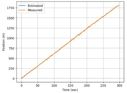
Linear Position-Time Path
- We begin with the simplest example of a linear position-time path. We need to estimate both position and velocity vs time using the following KF algorithm
import numpy as np
from numpy.linalg import inv
import matplotlib.pyplot as plt
def getMeasurement(updateNumber):
    if updateNumber == 1:
      getMeasurement.currentPosition = 0
      getMeasurement.currentVelocity = 60 # m/s

    dt = 0.1

    w = 8 * np.random.randn(1)
    v = 8 * np.random.randn(1)

    z = getMeasurement.currentPosition + getMeasurement.currentVelocity*dt + v
    getMeasurement.currentPosition = z - v
    getMeasurement.currentVelocity = 60 + w
    return [z, getMeasurement.currentPosition, getMeasurement.currentVelocity]
def filter(z, updateNumber):
    dt = 0.1
    # Initialize State
    if updateNumber == 1:
        filter.x = np.array([[0],
                            [20]])
        filter.P = np.array([[5, 0],
                                 [0, 5]])

        filter.A = np.array([[1, dt],
                             [0, 1]])
        filter.H = np.array([[1, 0]])
        filter.HT = np.array([[1],
                              [0]])
        filter.R = 10
        filter.Q = np.array([[1, 0],
                             [0, 3]])

    # Predict State Forward
    x_p = filter.A.dot(filter.x)
    # Predict Covariance Forward
    P_p = filter.A.dot(filter.P).dot(filter.A.T) + filter.Q
    # Compute Kalman Gain
    S = filter.H.dot(P_p).dot(filter.HT) + filter.R
    K = P_p.dot(filter.HT)*(1/S)

    # Estimate State
    residual = z - filter.H.dot(x_p)
    filter.x = x_p + K*residual

    # Estimate Covariance
    filter.P = P_p - K.dot(filter.H).dot(P_p)

    return [filter.x[0], filter.x[1], filter.P];
dt = 0.1
t = np.linspace(0, 10, num=300)
numOfMeasurements = len(t)

measTime = []
measPos = []
measDifPos = []
estDifPos = []
estPos = []
estVel = []
posBound3Sigma = []

for k in range(1,numOfMeasurements):
        z = getMeasurement(k)
        # Call Filter and return new State
        f = filter(z[0], k)
        # Save off that state so that it could be plotted
        measTime.append(k)
        measPos.append(z[0])
        measDifPos.append(z[0]-z[1])
        estDifPos.append(f[0]-z[1])
        estPos.append(f[0])
        estVel.append(f[1])
        posVar = f[2]
        posBound3Sigma.append(3*np.sqrt(posVar[0][0]))
- Plotting measured and estimated positions
plt.plot(estPos,label='Estimated')
plt.plot(measPos,label='Measured')
plt.ylabel('Position (m)')
plt.xlabel('Time (sec)')
plt.legend()
plt.grid()
- Plotting measured and estimated position differences
plt.plot(measDifPos,label='Measured')
plt.plot(estDifPos,label='Estimated',lw=4)
plt.ylabel('DifPos (m)')
plt.xlabel('Time (sec)')
plt.legend()
plt.grid()

- Estimated velocity
plt.plot(estVel)
plt.title('Estimated Velocity (km/h)')
plt.xlabel('Time (sec)')
plt.legend()
plt.grid()

- The plots generated by this example clearly show that the KF is working.
Parabolic Position-Time Path
- Let’s look at the parabolic position-time path using the KF algorithm
import numpy as np
import matplotlib.pyplot as plt
n=100
sz = (n) # size of array
t = np.linspace(0,10,n)
x = t + 2*t**2 # truth function
z = x + np.random.normal(0,7.5,size=sz) # noise

Q = 1e-3 # process variance

# allocate space for arrays
xhat=np.zeros(sz)      # a posteri estimate of x
P=np.zeros(sz)         # a posteri error estimate
xhatminus=np.zeros(sz) # a priori estimate of x
Pminus=np.zeros(sz)    # a priori error estimate
K=np.zeros(sz)         # Kalman gain

R = 0.03**2 # estimate of measurement variance


xhat[0] = 0.0
P[0] = 1.0

for i in range(1,n):

  xhatminus[i] = xhat[i-1]
  Pminus[i] = P[i-1]+Q


  K[i] = Pminus[i]/( Pminus[i]+R )
  xhat[i] = xhatminus[i]+K[i]*(z[i]-xhatminus[i])
  P[i] = (1-K[i])*Pminus[i]

plt.figure()
plt.plot(t, z,'k+',label='noisy measurements')
plt.plot(t, xhat,'b-',label='a posteri estimate')
plt.plot(t,x,color='g',label='truth value')
plt.legend()
plt.xlabel('Time')
plt.ylabel('Position')
plt.grid()

plt.show()
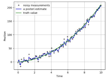
- It appears that KF still provides a reasonable approximation of the true path.
Extended Kalman Filter (EKF)
- Let’s consider the example of tracking a robot in circular motion using the Extended Kalman Filter (EKF) class
import numpy as np
import matplotlib.pyplot as plt
import math

class Filter:
    def __init__(self, var=None):
        self.filter = var
        self.filter.predict()

    def get_point(self):
        return self.filter.x[0:2].flatten()

    def predict_point(self, measurement):

        self.filter.predict()
        self.filter.update(measurement)
        return self.get_point()


class ExtendedKalmanFilter:
    def __init__(self,sigma,u,dt):
        self.x = np.array([0.,  # x
                           0.,  # y
                           0.,  # orientation
                           0.]).reshape(-1, 1)  # linear velocity

        self.u = u
        self.dt = dt
        self.p = np.diag([999. for i in range(4)])
        self.q = np.diag([0.1 for i in range(4)])
        self.r = np.diag([sigma, sigma])
        self.jf = np.diag([1. for i in range(4)])
        self.jg = np.array([[1., 0., 0., 0.],
                            [0., 1., 0., 0.]])
        self.h = np.array([[1., 0., 0., 0.],
                           [0., 1., 0., 0.]])
        self.z = np.array([0.,
                           0.]).reshape(-1, 1)

    def predict(self):
        x, y, phi, v = self.x
        vt, wt = self.u
        dT = self.dt

        new_x = x + vt * np.cos(phi) * dT
        new_y = y + vt * np.sin(phi) * dT
        new_phi = phi + wt * dT
        new_v = vt

        self.x[0]=new_x
        self.x[1]=new_y
        self.x[2]=new_phi
        self.x[3]=new_v

        self.jf[0][2] = -v * np.sin(phi) * dT
        self.jf[0][3] = v * np.cos(phi) * dT
        self.jf[1][2] = v * np.cos(phi) * dT
        self.jf[1][3] = v * np.sin(phi) * dT

        # p-prediction:
        self.p = self.jf.dot(self.p).dot(self.jf.transpose()) + self.q

    def update(self, measurement):
        z = np.array(measurement).reshape(-1, 1)
        y = z - self.h.dot(self.x)

        s = self.jg.dot(self.p).dot(self.jg.transpose()) + self.r
        k = self.p.dot(self.jg.transpose()).dot(np.linalg.inv(s))

        self.x = self.x + k.dot(y)
        self.p = (np.eye(4) - k.dot(self.h)).dot(self.p)

def action(parfilter, measurements):
    result = []
    for i in range(len(measurements)):
        m = measurements[i]
        pred = parfilter.predict_point(m)
        result.append(pred)

    return result

def create_artificial_circle_data(radius,dt,u,sigma):
    measurements = []
    vt, wt = u
    phi = np.arange(0, 2*math.pi, wt * dt)
    x = radius * np.cos(phi) + sigma * np.random.randn(len(phi))
    y = radius * np.sin(phi) + sigma * np.random.randn(len(phi))

    measurements += [[x, y] for x, y in zip(x, y)]
    return measurements

def plot(measurements, result, deadreckon_results):
    plt.figure("Extended Kalman Filter Visualization")
    plt.scatter([x[0] for x in measurements], [x[1] for x in measurements], c='red', label='GPS Position', alpha=0.3,s=4)
    plt.scatter([x[0] for x in result], [x[1] for x in result], c='blue', label='Kalman filter estimate Position', alpha=0.3, s=4,marker='x')
    plt.scatter([x[0] for x in deadreckon_results], [x[1] for x in deadreckon_results], c='black', label='dead reckoning Position', alpha=0.3, s=4,marker='x')
    plt.legend()
    plt.grid('on')
    plt.title("Circular Motion Robot and Kalman Filter Prediction")
    plt.xlabel("X-axis")
    plt.ylabel("Y-axis")
    plt.xlim(-10, 10)
    plt.ylim(-10, 10)
    plt.tight_layout()
    plt.show()

def deadReckoning(robo, u, dt):
    initial_state = robo.x
    vt, wt = u
    x=vt/wt
    y=0
    phi=math.pi/2
    x_list=[]
    y_list=[]
    phi_list=[]
    result = []
    T = 2 * math.pi / wt
    for i in range(int(T/dt)):
        new_x = x + vt * np.cos(phi) * dt
        new_y = y + vt * np.sin(phi) * dt
        new_phi = phi + wt * dt
        x = new_x
        y = new_y
        phi = new_phi
        # new_v = vt

        x_list.append(new_x)
        y_list.append(new_y)
        phi_list.append(new_phi)
    result += [[p, q] for p, q in zip(x_list, y_list)]

    return result
- Running the EKF code with sigma=0.5 and dt=0.001
if __name__ == '__main__':
    input_u = [10, 2]
    radiusOfCircle = input_u[0] / input_u[1]
    robot = ExtendedKalmanFilter(sigma=0.5, u=input_u, dt=0.001)
    robotController = Filter(robot)
    deadreckon_results=deadReckoning(robo=robot, u=input_u, dt=0.001)
    measurementGPS = create_artificial_circle_data(radius=radiusOfCircle,u=input_u, dt=0.001, sigma=0.5)
    results = action(robotController, measurementGPS)
    plot(measurementGPS, results, deadreckon_results)

- Running the above code with sigma=0.9 and dt=0.001

- Running the above code with sigma=0.9 and dt=0.01
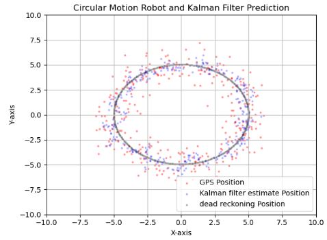
- Here we measure a circular (polar) movement in a Cartesian plane. The rotation gives an acceleration in X and Y and it is missing in the F matrix. We need to update the F matrix to include the complete physical model including acceleration.
- As any other KF algorithm, the EKF uses the state-to-measurement transformation to convert the system state estimate from the state space to the measurement space.
- In general, this test demonstrates the exceptional GPS noise robustness of EKF. It also highlights the importance of Q (model process covariance).
Tracking the Bike’s Path
- What about utilizing the noisy GPS signals to estimate the bike’s path? Does the implemented algorithm yield accurate knowledge of the bike’s position at any given time, including the associated velocity and acceleration information?
- Calculating the exact trajectory
import numpy as np

from numpy import pi, cos, sin, sqrt, diag
from numpy.linalg import inv
from numpy.random import randn


t = np.linspace(0, 2*pi, 100)
dt = t[1] - t[0]

print (dt)
0.06346651825433926

# position
x = 2*cos(t)
y = sin(2*t)

# velocity
dxdt = -2*sin(t)
dydt = 2*cos(2*t)

# accel
d2xdt2 = -2*cos(t)
d2ydt2 = -4*sin(2*t)

# jerk
d3xdt3 = 2*sin(t)
d3ydt3 = -8*cos(2*t)
- Plotting the exact trajectory
plt.plot(x,y)
plt.xlabel('X')
plt.ylabel('Y')
plt.title('TRAJECTORY')

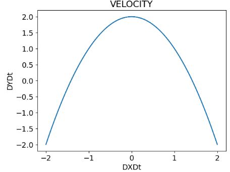
- Plotting the exact velocity
plt.plot(dxdt,dydt)
plt.xlabel('DXDt')
plt.ylabel('DYDt')
plt.title('VELOCITY')
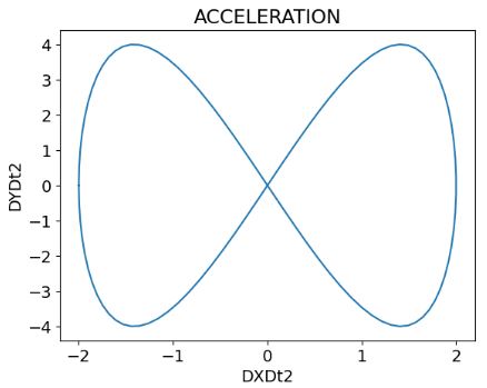
- Plotting the exact acceleration
plt.plot(d2xdt2,d2ydt2)
plt.xlabel('DXDt2')
plt.ylabel('DYDt2')
plt.title('ACCELERATION')
- Plotting the exact jerk
plt.plot(d3xdt3,d3ydt3)
plt.title('RATE OF ACCELERATION (JERK)')
plt.xlabel('DXDt3')
plt.ylabel('DYDt3')

- Calculating the angular speed and generating synthetic GPS measurements with noise
# angular speed (scalar)
omega = (dxdt*d2ydt2 - dydt*d2xdt2) / (dxdt**2 + dydt**2)

# speed (scalar)
speed = sqrt(dxdt**2 + dydt**2)

# measurement error
gps_sig = 0.1
omega_sig = 0.3
speed_sig = 0.1

# noisy measurements
x_gps = x + gps_sig * randn(*x.shape)
y_gps = y + gps_sig * randn(*y.shape)
omega_sens = omega + omega_sig * randn(*omega.shape)
speed_sens = speed + speed_sig * randn(*speed.shape)
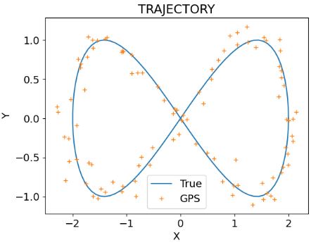
- Plotting the exact trajectory and the synthetic GPS data
plt.plot(x,y)
plt.plot(x_gps,y_gps,'+')
plt.legend(['True', 'GPS'])
plt.title('TRAJECTORY')
plt.xlabel('X')
plt.ylabel('Y')
- Plotting the exact velocity and the velocity sensor data
plt.plot(t,speed)
plt.plot(t,speed_sens,'+')
plt.legend(['True', 'Sensor'])
plt.title('SPEED V')
plt.xlabel('VX')
plt.ylabel('VY')

- Plotting the exact angular speed and the corresponding sensor measurements
plt.plot(t,omega)
plt.plot(t,omega_sens,'+')
plt.legend(['True', 'GPS'])
plt.title('ANGULAR SPEED W')
plt.xlabel('WX')
plt.ylabel('WY')

- Applying the KF algorithm to the above data
A = np.array([
    [1, dt, (dt**2)/2, 0, 0, 0],
    [0, 1, dt, 0, 0, 0],
    [0, 0, 1, 0, 0, 0],
    [0, 0, 0, 1, dt, (dt**2)/2],
    [0, 0, 0, 0, 1, dt],
    [0, 0, 0, 0, 0, 1],
    ])
Q1 = np.array([(dt**3)/6, (dt**2)/2, dt, 0, 0, 0])
Q1 = np.expand_dims(Q1, 1)
Q2 = np.array([0, 0, 0, (dt**3)/6, (dt**2)/2, dt])
Q2 = np.expand_dims(Q2, 1)

j_var = max(np.var(d3xdt3), np.var(d3ydt3))
Q = j_var * (Q1 @ Q1.T + Q2 @ Q2.T)
H = np.array([
    [1, 0, 0, 0, 0, 0],
    [0, 0, 0, 1, 0, 0],
    ])
R = diag(np.array([gps_sig**2, gps_sig**2]))
x_init = np.array([x[0], dxdt[0], d2xdt2[0], y[0], dydt[0], d2ydt2[0]])
P_init = 0.01 * np.eye(len(x_init))  # small initial prediction error
# create an observation vector of noisy GPS signals
observations = np.array([x_gps, y_gps]).T

# matrix dimensions
nx = Q.shape[0]
ny = R.shape[0]
nt = observations.shape[0]

# allocate identity matrix for re-use
Inx = np.eye(nx)

# allocate result matrices
x_pred = np.zeros((nt, nx))      # prediction of state vector
P_pred = np.zeros((nt, nx, nx))  # prediction error covariance matrix
x_est = np.zeros((nt, nx))       # estimation of state vector
P_est = np.zeros((nt, nx, nx))   # estimation error covariance matrix
K = np.zeros((nt, nx, ny))       # Kalman Gain

# set initial prediction
x_pred[0] = x_init
P_pred[0] = P_init

# for each time-step...
for i in range(nt):

    # prediction stage
    if i > 0:
        x_pred[i] = A @ x_est[i-1]
        P_pred[i] = A @ P_est[i-1] @ A.T + Q

    # estimation stage
    y_obs = observations[i]
    K[i] = P_pred[i] @ H.T @ inv((H @ P_pred[i] @ H.T) + R)
    x_est[i] = x_pred[i] + K[i] @ (y_obs - H @ x_pred[i])
    P_est[i] = (Inx - K[i] @ H) @ P_pred[i]
- Comparing the exact and the KF estimated trajectories
plt.plot(x,y)
plt.plot(x_est[:, 0],x_est[:, 3])
plt.legend(['True', 'Estimate'])
plt.title('TRAJECTORY')
plt.xlabel('X')
plt.ylabel('Y')

- By plotting the X and Y position estimations, we can see that the KF performed reasonably well.
- One problem with the above KF algorithm is that it only works for models with purely linear relationships. It was fine for the GPS-only example above, but as soon as we try to assimilate data from the other two sensors, the method falls apart. This is because the speed and angular speed measurements have non-linear relationships with the bike state vector.
- Now let’s apply the Extended Kalman Filter (EKF) algorithm to assimilate the GPS, speedometer (velocity), and gyroscope (acceleration) signals with our predictive model
#Example 2: Use the Extended Kalman Filter to Assimilate All Sensors
def eval_h(x_pred):

    # expand prediction of state vector
    px, vx, ax, py, vy, ay = x_pred

    # compute angular vel
    w = (vx*ay - vy*ax) / (vx**2 + vy**2)

    # compute speed
    s = sqrt(vx**2 + vy**2)

    return np.array([px, py, w, s])

def eval_H(x_pred):

    # expand prediction of state vector
    px, vx, ax, py, vy, ay = x_pred
    V2 = vx**2 + vy**2

    # angular vel partial derivs
    dwdvx = (V2*ay - 2*vx*(vx*ay-vy*ax)) / (V2**2)
    dwdax = -vy / V2
    dwdvy = (-V2*ax - 2*vy*(vx*ay-vy*ax)) / (V2**2)
    dwday = vx / V2

    # speed partial derivs
    dsdvx = vx / sqrt(V2)
    dsdvy = vy / sqrt(V2)

    return np.array([
        [1, 0, 0, 0, 0, 0],
        [0, 0, 0, 1, 0, 0],
        [0, dwdvx, dwdax, 0, dwdvy, dwday],
        [0, dsdvx, 0, 0, dsdvy, 0],
        ])
# redefine R to include speedometer and gyro variances
R = diag(np.array([gps_sig**2, gps_sig**2, omega_sig**2, speed_sig**2]))
# create an observation vector of all noisy signals
observations = np.array([x_gps, y_gps, omega_sens, speed_sens]).T

# matrix dimensions
nx = Q.shape[0]
ny = R.shape[0]
nt = observations.shape[0]

# allocate identity matrix for re-use
Inx = np.eye(nx)

# allocate result matrices
x_pred = np.zeros((nt, nx))      # prediction of state vector
P_pred = np.zeros((nt, nx, nx))  # prediction error covariance matrix
x_est = np.zeros((nt, nx))       # estimation of state vector
P_est = np.zeros((nt, nx, nx))   # estimation error covariance matrix
K = np.zeros((nt, nx, ny))       # Kalman Gain

# set initial prediction
x_pred[0] = x_init
P_pred[0] = P_init

# for each time-step...
for i in range(nt):

    # prediction stage
    if i > 0:
        x_pred[i] = A @ x_est[i-1]
        P_pred[i] = A @ P_est[i-1] @ A.T + Q

    # estimation stage
    y_obs = observations[i]
    y_pred = eval_h(x_pred[i])
    H_pred = eval_H(x_pred[i])
    K[i] = P_pred[i] @ H_pred.T @ inv((H_pred @ P_pred[i] @ H_pred.T) + R)
    x_est[i] = x_pred[i] + K[i] @ (y_obs - y_pred)
    P_est[i] = (Inx - K[i] @ H_pred) @ P_pred[i]
- Comparing the exact and the EKF estimated trajectories
plt.plot(x,y)
plt.plot(x_est[:, 0],x_est[:, 3])
plt.legend(['True', 'Estimate'])
plt.title('TRAJECTORY')
plt.xlabel('X')
plt.ylabel('Y')

- By plotting the X and Y position estimations, we can see that the EKF performed even better than the KF.
- Bottom line: it is very instructive working through the process of mocking up the bike scenario and then applying the KF and EKF to the artificial data.
Unscented Kalman Filter (UKF)
- In this section, we will evaluate the Unscented Kalman filter (UKF) that incorporates the unscented transformation into the regular KF algorithm. It consists of the following two steps:
1. Prediction Step
- Calculating Sigma Points
- Calculating Associated Weights
- Nonlinear Function Propagation
- Calculating Weighted Mean and Covariance
- Augmenting State and Covariance
2. Correction Step
- Propagating Predicted Sigma Points
- Cross-Correlation Calculation
- Kalman Gain Calculation
- State and Covariance Update
- Running the corresponding code
import numpy as np
import matplotlib.pyplot as plt
import scipy.stats as stats
import math
import sys
def augment_vectors(x, v):
    return np.row_stack((x, v))

def augment_covariances(P, Q):
    prows, pcols = np.shape(P)[0], np.shape(P)[1]
    qrows, qcols = np.shape(Q)[0], np.shape(Q)[1]

    nrows = prows + qrows
    ncols = pcols + qcols

    Pa = np.zeros((nrows, ncols))
    Pa[0:prows, 0:pcols] = P
    Pa[prows:nrows, pcols:ncols] = Q

    return Pa
x = np.array([[1.], [2.]])
v = np.array([[3.], [4.]])

P = np.array([[1., 1.], [1., 1.]])
Q = np.array([[2., 2.], [2., 2.]])

xa = augment_vectors(x, v)
Pa = augment_covariances(P, Q)

print(xa)
print(Pa)
[[1.]
 [2.]
 [3.]
 [4.]]
[[1. 1. 0. 0.]
 [1. 1. 0. 0.]
 [0. 0. 2. 2.]
 [0. 0. 2. 2.]]
#Unscented Kalman Filter (UKF)
class UKF(object):
    def __init__(self, dim_x, dim_z, Q, R, kappa=0.0):

        '''
        UKF class constructor
        inputs:
            dim_x : state vector x dimension
            dim_z : measurement vector z dimension

        - step 1: setting dimensions
        - step 2: setting number of sigma points to be generated
        - step 3: setting scaling parameters
        - step 4: calculate scaling coefficient for selecting sigma points
        - step 5: calculate weights
        '''

        # setting dimensions
        self.dim_x = dim_x         # state dimension
        self.dim_z = dim_z         # measurement dimension
        self.dim_v = np.shape(Q)[0]
        self.dim_n = np.shape(R)[0]
        self.dim_a = self.dim_x + self.dim_v + self.dim_n # assuming noise dimension is same as x dimension

        # setting number of sigma points to be generated
        self.n_sigma = (2 * self.dim_a) + 1

        # setting scaling parameters
        self.kappa = 3 - self.dim_a #kappa
        self.alpha = 0.001
        self.beta = 2.0

        alpha_2 = self.alpha**2
        self.lambda_ = alpha_2 * (self.dim_a + self.kappa) - self.dim_a

        # setting scale coefficient for selecting sigma points
        # self.sigma_scale = np.sqrt(self.dim_a + self.lambda_)
        self.sigma_scale = np.sqrt(self.dim_a + self.kappa)

        # calculate unscented weights
        # self.W0m = self.W0c = self.lambda_ / (self.dim_a + self.lambda_)
        # self.W0c = self.W0c + (1.0 - alpha_2 + self.beta)
        # self.Wi = 0.5 / (self.dim_a + self.lambda_)

        self.W0 = self.kappa / (self.dim_a + self.kappa)
        self.Wi = 0.5 / (self.dim_a + self.kappa)

        # initializing augmented state x_a and augmented covariance P_a
        self.x_a = np.zeros((self.dim_a, ))
        self.P_a = np.zeros((self.dim_a, self.dim_a))

        self.idx1, self.idx2 = self.dim_x, self.dim_x + self.dim_v

        self.P_a[self.idx1:self.idx2, self.idx1:self.idx2] = Q
        self.P_a[self.idx2:, self.idx2:] = R

        print(f'P_a = \n{self.P_a}\n')

    def predict(self, f, x, P):
        self.x_a[:self.dim_x] = x
        self.P_a[:self.dim_x, :self.dim_x] = P

        xa_sigmas = self.sigma_points(self.x_a, self.P_a)

        xx_sigmas = xa_sigmas[:self.dim_x, :]
        xv_sigmas = xa_sigmas[self.idx1:self.idx2, :]

        y_sigmas = np.zeros((self.dim_x, self.n_sigma))
        for i in range(self.n_sigma):
            y_sigmas[:, i] = f(xx_sigmas[:, i], xv_sigmas[:, i])

        y, Pyy = self.calculate_mean_and_covariance(y_sigmas)

        self.x_a[:self.dim_x] = y
        self.P_a[:self.dim_x, :self.dim_x] = Pyy

        return y, Pyy, xx_sigmas

    def correct(self, h, x, P, z):
        self.x_a[:self.dim_x] = x
        self.P_a[:self.dim_x, :self.dim_x] = P

        xa_sigmas = self.sigma_points(self.x_a, self.P_a)

        xx_sigmas = xa_sigmas[:self.dim_x, :]
        xn_sigmas = xa_sigmas[self.idx2:, :]

        y_sigmas = np.zeros((self.dim_z, self.n_sigma))
        for i in range(self.n_sigma):
            y_sigmas[:, i] = h(xx_sigmas[:, i], xn_sigmas[:, i])

        y, Pyy = self.calculate_mean_and_covariance(y_sigmas)

        Pxy = self.calculate_cross_correlation(x, xx_sigmas, y, y_sigmas)

        K = Pxy @ np.linalg.pinv(Pyy)

        x = x + (K @ (z - y))
        P = P - (K @ Pyy @ K.T)

        return x, P, xx_sigmas


    def sigma_points(self, x, P):

        '''
        generating sigma points matrix x_sigma given mean 'x' and covariance 'P'
        '''

        nx = np.shape(x)[0]

        x_sigma = np.zeros((nx, self.n_sigma))
        x_sigma[:, 0] = x

        S = np.linalg.cholesky(P)

        for i in range(nx):
            x_sigma[:, i + 1]      = x + (self.sigma_scale * S[:, i])
            x_sigma[:, i + nx + 1] = x - (self.sigma_scale * S[:, i])

        return x_sigma


    def calculate_mean_and_covariance(self, y_sigmas):
        ydim = np.shape(y_sigmas)[0]

        # mean calculation
        y = self.W0 * y_sigmas[:, 0]
        for i in range(1, self.n_sigma):
            y += self.Wi * y_sigmas[:, i]

        # covariance calculation
        d = (y_sigmas[:, 0] - y).reshape([-1, 1])
        Pyy = self.W0 * (d @ d.T)
        for i in range(1, self.n_sigma):
            d = (y_sigmas[:, i] - y).reshape([-1, 1])
            Pyy += self.Wi * (d @ d.T)

        return y, Pyy

    def calculate_cross_correlation(self, x, x_sigmas, y, y_sigmas):
        xdim = np.shape(x)[0]
        ydim = np.shape(y)[0]

        n_sigmas = np.shape(x_sigmas)[1]

        dx = (x_sigmas[:, 0] - x).reshape([-1, 1])
        dy = (y_sigmas[:, 0] - y).reshape([-1, 1])
        Pxy = self.W0 * (dx @ dy.T)
        for i in range(1, n_sigmas):
            dx = (x_sigmas[:, i] - x).reshape([-1, 1])
            dy = (y_sigmas[:, i] - y).reshape([-1, 1])
            Pxy += self.Wi * (dx @ dy.T)

        return Pxy
x0 = np.array([1.0, 2.0])
P0 = np.array([[1.0, 0.0], [0.0, 1.0]])
Q = np.array([[0.5, 0.0], [0.0, 0.5]])

z = np.array([1.2, 1.8])
R = np.array([[0.3, 0.0], [0.0, 0.3]])
def f(x, v):
    return (x + v)

def h(x, n):
    return (x + n)

nx = np.shape(x)[0]
nz = np.shape(z)[0]
nv = np.shape(x)[0]
nn = np.shape(z)[0]

ukf = UKF(dim_x=nx, dim_z=nz, Q=Q, R=R, kappa=(3 - nx))

x1, P1, _ = ukf.predict(f, x0, P0)

print(f'x = \n{x1.round(5)}\n')
print(f'P = \n{P1.round(5)}\n')

x2, P2, _ = ukf.correct(h, x1, P1, z)

print(f'x = \n{x2.round(5)}\n')
print(f'P = \n{P2.round(5)}\n')

P_a =
[[0.  0.  0.  0.  0.  0. ]
 [0.  0.  0.  0.  0.  0. ]
 [0.  0.  0.5 0.  0.  0. ]
 [0.  0.  0.  0.5 0.  0. ]
 [0.  0.  0.  0.  0.3 0. ]
 [0.  0.  0.  0.  0.  0.3]]

x =
[1. 2.]

P =
[[1.5 0. ]
 [0.  1.5]]

x =
[1.16667 1.83333]

P =
[[ 0.25 -0.  ]
 [-0.    0.25]]
def KF_predict(F, x, P, Q):
    x = (F @ x)
    P = F @ P @ F.T + Q
    return x, P

def KF_correct(H, z, R, x, P):
    Pxz = P @ H.T
    S = H @ P @ H.T + R

    K = Pxz @ np.linalg.pinv(S)

    x = x + K @ (z - H @ x)
    I = np.eye(P.shape[0])
    P = (I - K @ H) @ P
    return x, P

F = np.array([[1.0, 0.0], [0.0, 1.0]])
H = np.array([[1.0, 0.0], [0.0, 1.0]])

x1, P1 = KF_predict(F, x0, P0, Q)

print(f'x = \n{x1.round(5)}\n')
print(f'P = \n{P1.round(5)}\n')

x2, P2 = KF_correct(H, x1, P1, z, R)

print(f'x = \n{x2.round(5)}\n')
print(f'P = \n{P2.round(5)}\n')
x =
[1. 2.]

P =
[[1.5 0. ]
 [0.  1.5]]

x =
[1.16667 1.83333]

P =
[[0.25 0.  ]
 [0.   0.25]]
def f_2(x, nu):
    xo = np.zeros((np.shape(x)[0],))
    xo[0] = x[0] + x[2] + nu[0]
    xo[1] = x[1] + x[3] + nu[1]
    xo[2] = x[2] + nu[2]
    xo[3] = x[3] + nu[3]
    return xo
class RangeMeasurement:
    def __init__(self, position):
        self.range = np.sqrt(position[0]**2 + position[1]**2)
        self.bearing = np.arctan(position[1] / (position[0] + sys.float_info.epsilon))
        self.position = np.array([position[0],position[1]])

    def actual_position(self):
        return self.position

    def asArray(self):
        return np.array([self.range,self.bearing])

    def show(self):
        print(f'range: {self.range}')
        print(f'bearing: {self.bearing}')

measurement = RangeMeasurement((10.7, 5.6)) # ground-truth
measurement.show()
range: 12.076837334335508
bearing: 0.4821640110688151
def h_2(x, n):
    '''
    nonlinear measurement model for range sensor
    x : input state vector [2 x 1] ([0]: p_x, [1]: p_y)
    z : output measurement vector [2 x 1] ([0]: range, [1]: bearing )
    '''
    z = np.zeros((2,))
    px = x[0] + n[0]
    py = x[1] + n[1]

    z[0] = np.sqrt(px**2 + py**2)
    z[1] = np.arctan(py / (px + sys.float_info.epsilon))
    return z
x0 = np.array([2.0, 1.0, 0., 0.])

P0 = np.array([[0.01, 0.0, 0.0, 0.0],
              [0.0, 0.01, 0.0, 0.0],
              [0.0, 0.0, 0.05, 0.0],
              [0.0, 0.0, 0.0, 0.05]])

Q = np.array([[0.05, 0.0, 0.0, 0.0],
              [0.0, 0.05, 0.0, 0.0],
              [0.0, 0.0, 0.1, 0.0],
              [0.0, 0.0, 0.0, 0.1]])

R = np.array([[0.01, 0.0],
              [0.0, 0.01]])

z = np.array([2.5, 0.05])

nx = np.shape(x0)[0]
nz = np.shape(R)[0]
nv = np.shape(x0)[0]
nn = np.shape(R)[0]

ukf = UKF(dim_x=nx, dim_z=nz, Q=Q, R=R, kappa=(3 - nx))

x, P, _ = ukf.predict(f_2, x0, P0)

print(f'x = \n {x.round(3)}')
print(f'P = \n {P.round(3)}')

x, P, _ = ukf.correct(h_2, x, P, z)

print(f'x = \n {x.round(3)}')
print(f'P = \n {P.round(3)}')
P_a =
[[0.   0.   0.   ... 0.   0.   0.  ]
 [0.   0.   0.   ... 0.   0.   0.  ]
 [0.   0.   0.   ... 0.   0.   0.  ]
 ...
 [0.   0.   0.   ... 0.1  0.   0.  ]
 [0.   0.   0.   ... 0.   0.01 0.  ]
 [0.   0.   0.   ... 0.   0.   0.01]]

x =
 [2. 1. 0. 0.]
P =
 [[ 0.11  0.    0.05 -0.  ]
 [ 0.    0.11 -0.    0.05]
 [ 0.05 -0.    0.15  0.  ]
 [-0.    0.05  0.    0.15]]
x =
 [ 2.554  0.356  0.252 -0.293]
P =
 [[ 0.01  -0.001  0.005 -0.   ]
 [-0.001  0.01  -0.     0.005]
 [ 0.005 -0.     0.129 -0.   ]
 [-0.     0.005 -0.     0.129]]
# prepare helper functions for visualizing the ellipses
from matplotlib.patches import Ellipse

def create_covariance_ellipse(pos, cov):
    # https://www.visiondummy.com/2014/04/draw-error-ellipse-representing-covariance-matrix
    eig_values, eig_vectors = np.linalg.eig(cov)

    scale_95 = np.sqrt(5.991)
    radius_1 = scale_95 * eig_values[0]
    radius_2 = scale_95 * eig_values[1]
    angle = np.arctan2(eig_vectors[1, 1], eig_vectors[0, 1])

    return radius_1, radius_2, angle

def draw_ellipse(ax, mu, radius_1, radius_2, angle, color):
    # https://matplotlib.org/stable/gallery/shapes_and_collections/ellipse_demo.html
    ellipse = Ellipse(
        mu,
        width=radius_1 * 2,
        height=radius_2 * 2,
        angle=np.rad2deg(angle) + 90,
        facecolor=color,
        alpha=0.4)
    ax.add_artist(ellipse)
    return ax

def plot_ellipse(ax, x, P, color):
    x = x[0:2].reshape(2,)
    P = P[0:2, 0:2]
    r1, r2, angle = create_covariance_ellipse(x, P)
    draw_ellipse(ax, x, r1, r2, angle, color)

def get_correlated_dataset(n, cov, mu, scale):
    # https://carstenschelp.github.io/2018/09/14/Plot_Confidence_Ellipse_001.html
    latent = np.random.randn(n, 2)
    cov = latent.dot(cov)
    scaled = cov * scale
    scaled_with_offset = scaled + mu
    # return x and y of the new, correlated dataset
    return scaled_with_offset[:, 0], scaled_with_offset[:, 1]

def plot_samples(ax, samples_num, x, P, color, markersize, label):
    scale = 1, 1
    x, y = get_correlated_dataset(samples_num, P, x, scale)
    ax.scatter(x, y, s=markersize, marker='x', c=color, label=label)

def plot_mean(ax, x, size, color, label):
    ax.scatter(x[0], x[1], s=size, marker='o', c=color, label=label)

def plot_state(ax, x, P, samples_num, markersize, color, label):
    x = x[0:2].reshape(2,)
    P = P[0:2, 0:2]

    plot_ellipse(ax, x, P, color)
    plot_samples(ax, samples_num, x, P, color, markersize, label+'_possibilities')
    plot_mean(ax, x, 200, color, label+'_mean')

def create_viewer(title, xlabel, ylabel, xlim=None, ylim=None):
    fig, viewer = plt.subplots(figsize=(24, 12))

    viewer.set_title(title, fontsize=22, color='green', fontweight='bold')

    viewer.axvline(c='grey', lw=2)
    viewer.axhline(c='grey', lw=2)

    viewer.set_xlabel(xlabel, fontsize=22, fontweight ='bold')
    viewer.set_ylabel(ylabel, fontsize=22, fontweight ='bold')

    if (xlim != None):
        viewer.set_xlim(xlim[0], xlim[1])

    if (ylim != None):
        viewer.set_ylim(ylim[0], ylim[1])

    return viewer

def visualize_estimate(viewer, label, color, x, P):
    plot_state(viewer, x=x, P=P, samples_num=500, markersize=16, color=color, label=label)

def update_plotter():
    plt.grid(visible=True)
    plt.legend(loc='upper left')
    plt.show()
x0 = np.array([10., 5., 0., 0.])

P0 = np.array([[0.3, 0.1, 0.0, 0.0],
              [0.1, 0.3, 0.0, 0.0],
              [0.0, 0.0, 0.1, 0.0],
              [0.0, 0.0, 0.0, 0.1]])

Q = np.array([[0.05, 0.0, 0.0, 0.0],
              [0.0, 0.05, 0.0, 0.0],
              [0.0, 0.0, 0.1, 0.0],
              [0.0, 0.0, 0.0, 0.1]])

z = measurement.asArray()
R = np.array([[0.1, 0.0],[0.0, 0.1]])

nx = np.shape(x0)[0]
nz = np.shape(z)[0]
nv = np.shape(x0)[0]
nn = np.shape(z)[0]

ukf = UKF(dim_x=nx, dim_z=nz, Q=Q, R=R, kappa=(3 - nx))


print('=====Iteration 1====')
x, P, x_sigmas = ukf.correct(h_2, x0, P0, z)
print(f'x = \n{x.round(3)}\n')
print(f'P = \n{P.round(3)}\n')
print('\n\n')
P_a =
[[0.  0.  0.  ... 0.  0.  0. ]
 [0.  0.  0.  ... 0.  0.  0. ]
 [0.  0.  0.  ... 0.  0.  0. ]
 ...
 [0.  0.  0.  ... 0.1 0.  0. ]
 [0.  0.  0.  ... 0.  0.1 0. ]
 [0.  0.  0.  ... 0.  0.  0.1]]

=====Iteration 1====
x =
[10.548  5.476  0.     0.   ]

P =
[[0.073 0.007 0.    0.   ]
 [0.007 0.073 0.    0.   ]
 [0.    0.    0.1   0.   ]
 [0.    0.    0.    0.1  ]]
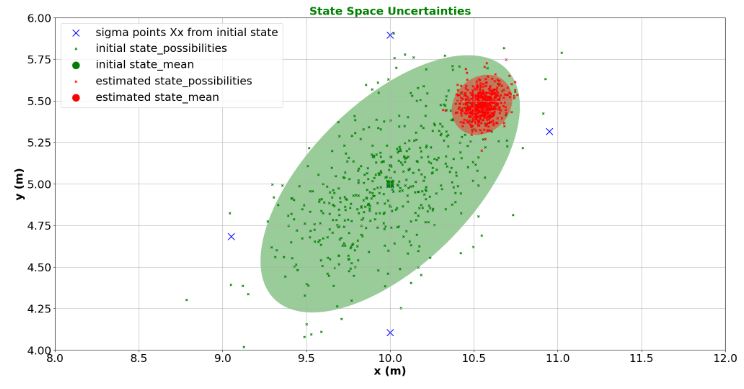
- Plotting State Space Uncertainties
viewer = create_viewer('State Space Uncertainties', 'x (m)', 'y (m)', xlim=(8,12), ylim=(4,6))

print(x_sigmas[:2, :5])

sigma_xlist = x_sigmas[0, :]
sigma_ylist = x_sigmas[1, :]

viewer.scatter(sigma_xlist, sigma_ylist, s=180, marker='x', c='blue', label='sigma points Xx from initial state')

visualize_estimate(viewer, 'initial state', 'g', x0, P0)
visualize_estimate(viewer, 'estimated state', 'r', x, P)

update_plotter()

[[10.         10.9486833  10.         10.         10.        ]
 [ 5.          5.31622777  5.89442719  5.          5.        ]]
- Tracking Target Trajectory
# generate trajectory

trajectory = [[10.0, 5.0], [11.0, 5.3], [12.0, 5.5], [13.0, 6.0], [14.0, 6.8], [15.0, 6.3], [16.0, 6.5]]
trajectory = np.asarray(trajectory)

traj_xlist = trajectory[:, 0]
traj_ylist = trajectory[:, 1]

print(traj_xlist)
print(traj_ylist)

measurements = []
for pose in trajectory:
    meas = RangeMeasurement(pose)
    measurements.append(meas.asArray())

measurements = np.asarray(measurements)


x0 = np.array([10., 5., 0., 0.])

P0 = np.array([[0.1, 0.0, 0.0, 0.0],
              [0.0, 0.1, 0.0, 0.0],
              [0.0, 0.0, 0.1, 0.0],
              [0.0, 0.0, 0.0, 0.1]])

Q = np.array([[0.05, 0.0, 0.0, 0.0],
              [0.0, 0.05, 0.0, 0.0],
              [0.0, 0.0, 0.1, 0.0],
              [0.0, 0.0, 0.0, 0.1]])

R = np.array([[0.1, 0.0],[0.0, 0.1]])

nx = np.shape(x0)[0]
nz = np.shape(R)[0]
nv = np.shape(x0)[0]
nn = np.shape(R)[0]

ukf = UKF(dim_x=nx, dim_z=nz, Q=Q, R=R, kappa=(3 - nx))

viewer = create_viewer('Tracking Target Trajectory', 'x (m)', 'y (m)', xlim=(8,20), ylim=(4,8))
viewer.scatter(traj_xlist, traj_ylist, s=80, marker='o', c='blue', label='actual target poses')

x, P = x0, P0

estimates = []

for iteration, z in enumerate(measurements):
    x, P, _ = ukf.predict(f_2, x, P)
    x, P, _ = ukf.correct(h_2, x, P, z)
    visualize_estimate(viewer, f'', 'g', x, P)

    estimates.append(x)

estimates = np.asarray(estimates).T
print(estimates)

estimates_px = estimates[0, :]
estimates_py = estimates[1, :]

estimates_vx = estimates[2, :]
estimates_vy = estimates[3, :]

viewer.plot(estimates_px, estimates_py)

update_plotter()
[10. 11. 12. ... 14. 15. 16.]
[5.  5.3 5.5 ... 6.8 6.3 6.5]
P_a =
[[0.  0.  0.  ... 0.  0.  0. ]
 [0.  0.  0.  ... 0.  0.  0. ]
 [0.  0.  0.  ... 0.  0.  0. ]
 ...
 [0.  0.  0.  ... 0.1 0.  0. ]
 [0.  0.  0.  ... 0.  0.1 0. ]
 [0.  0.  0.  ... 0.  0.  0.1]]

[[ 9.99002177 10.75545459 11.81946368 ... 13.97015886 15.00954828
  15.99740642]
 [ 4.9949255   5.23829684  5.48105352 ...  6.68249639  6.47940462
   6.51869704]
 [-0.00399129  0.43554205  0.79264229 ...  1.01577438  1.0288903
   1.00587547]
 [-0.0020298   0.13822184  0.197749   ...  0.5713585   0.13736439
   0.08238877]]
- Plotting the estimated x-,y-velocity profile from UKF
viewer = create_viewer('Velocity Profile', 'iteration', 'velocity (m/s)')
plt.rcParams.update({'font.size': 22})
viewer.plot(estimates_vx, color = 'blue', label='x_velocity')
viewer.plot(estimates_vy, color = 'red', label='y_velocity')
update_plotter()

Industry Application in Dynamic Positioning System
- In this section, we will choose a real life scenario by working onboard a ship with Dynamic Positioning (DP) system. Here, KF is used to in order to estimate a stable DP information from multiple sensors such as GPS, wind, current, IMU sensors, acoustic transponders, etc.
- In order to simplify the problem, we use only position data (x and y axes) and follow these steps:
- Defining the time period and the actual position of the ship.
- Creating imaginary, noisy position measurements.
- Calculating related KF matrices and saving calculated measurements after KF is applied.
- Comparing actual data vs estimated positions.
#Kalman Filter in Dynamic Positioning System
import numpy as np
import pandas as pd
import math
import matplotlib.pyplot as plt
from numpy.linalg import inv

n_iters = 50

# Actual position of the ship
actual_x = 0
actual_y = 0

# Process noise covariance which is assumed to be a small value.
Q = np.full((2,2), 0.0001)
print('Q matrix: ', Q.shape, '\n\n', Q)
Q matrix:  (2, 2)

 [[0.0001 0.0001]
 [0.0001 0.0001]]

# Create 50 random x and y position measurements
x_pos = np.random.normal(0, 0.5, n_iters)
y_pos = np.random.normal(0, 0.5, n_iters)

# Combine the measurements in a matrix
measurements = np.stack((x_pos, y_pos), axis=1).reshape((n_iters,2,1))

print('Measurements: ', measurements.shape, '\n\n', measurements[0:5], '\n', '...')
Measurements:  (50, 2, 1)

 [[[-0.18828139]
  [ 0.41481874]]

 [[ 0.0424575 ]
  [ 0.32092219]]

 [[-0.26253112]
  [ 0.10642768]]

 [[-0.31451265]
  [-0.4752949 ]]

 [[ 0.81230049]
  [-0.4795513 ]]]
 ...
# Measurement noise covariance.
R = np.diag([0.25, 0.25])
print('R matrix: ', R.shape, '\n\n', R)
R matrix:  (2, 2)

 [[0.25 0.  ]
 [0.   0.25]]
# Creating empty matrices
x_hat = np.zeros((n_iters, 2,1))
P = np.zeros((n_iters,2,2))
x_hat_min = np.zeros((n_iters, 2,1))
P_min = np.zeros((n_iters,2,2))
K = np.zeros((n_iters,2,2))
# Initial state
x_hat[0] = [[0],[0]]

# Initial error covariance
P[0] = np.diag([1000.0, 1000.0])

print('x_hat[0]:\n\n', x_hat[0], '\n\n P[0] matrix: ', P[0].shape, '\n\n', P[0])
x_hat[0]:

 [[0.]
 [0.]]

 P[0] matrix:  (2, 2)

 [[1000.    0.]
 [   0. 1000.]]
# A matrix
A = np.array([[1.0, 0.0],
               [0.0, 1.0]])

# H matrix
H = np.eye(2)

# Unit matrix for Kalman gain
I = np.eye(2)

print('A matrix \n\n', A, '\n\n H matrix \n\n', H, '\n\n I matrix \n\n', I)
A matrix

 [[1. 0.]
 [0. 1.]]

 H matrix

 [[1. 0.]
 [0. 1.]]

 I matrix

 [[1. 0.]
 [0. 1.]]
for k in range(1, n_iters):
    # Calculating a priori estimate and error covariance
    x_hat_min[k] = A.dot(x_hat[k-1])
    P_min[k] = A.dot(P[k-1]).dot(A.T) + Q

    # Calculating Kalman gain
    S = H.dot(P_min[k]).dot(H.T) + R
    K[k] = P_min[k].dot(H.T).dot(inv(S))

    # Calculating a posteriori estimate and error covariance
    x_hat[k] = x_hat_min[k] + K[k].dot(measurements[k] - H.dot(x_hat_min[k]))
    P[k] = (I - K[k]).dot(P_min[k])
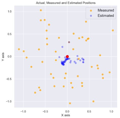
- Plotting Actual, Measured and Estimated Positions
plt.figure(figsize=(7,7))
for n in range(n_iters):
    plt.scatter(float(measurements[n][0]), float(measurements[n][1]),
                color='orange', label='measured position', alpha=0.7)
    plt.scatter(float(x_hat[n][0]), float(x_hat[n][1]),
                color='blue', label='kalman position', alpha=0.3)

plt.scatter(actual_x, actual_y, color='red', s=100, label='actual position')
plt.title('Actual, Measured and Estimated Positions')
plt.legend(['Measured', 'Estimated'], fontsize=14)
plt.xlabel('X axis')
plt.ylabel('Y axis');
- Plotting Actual, Measured and Estimated Positions on X axis
plt.figure(figsize=(10,5))
for n in range(n_iters):
    plt.scatter(x = n, y = measurements[n][0], label='measurements', color='orange', alpha=0.7)
    plt.scatter(x = n, y = x_hat[n][0], label='estimate after kalman', color='blue', alpha=0.5)
plt.axhline(actual_x, color='r', label='actual x position')
plt.title('Actual, Measured and Estimated Positions on X axis')
plt.xlabel('Number of Steps')
plt.ylabel('X Position')
- Plotting Actual, Measured and Estimated Positions on Y axis
plt.figure(figsize=(10,5))
for n in range(n_iters):
    plt.scatter(x = n, y = measurements[n][1], label='measurements', color='orange', alpha=0.7)
    plt.scatter(x = n, y = x_hat[n][1], label='estimate after kalman', color='blue', alpha=0.5)
plt.axhline(actual_x, color='r', label='actual x position')
plt.title('Actual, Measured and Estimated Positions on Y axis')
plt.xlabel('Number of Steps')
plt.ylabel('Y Position');

- Creating the following Plotly animation
# Creating a pandas dataframe for animation
x_position = []
y_position = []
data_type = []
n_steps = []

for n in range(n_iters):
    x_position.append(float(measurements[n][0]))
    y_position.append(float(measurements[n][1]))
    data_type.append('measured')
    n_steps.append(int(n))

for n in range(n_iters):
    x_position.append(float(x_hat[n][0]))
    y_position.append(float(x_hat[n][1]))
    data_type.append('estimated')
    n_steps.append(int(n))

df = pd.DataFrame({'x_position':x_position,
                   'y_position':y_position,
                   'data_type':data_type,
                   'n_steps':n_steps})

# Creating the animation
import plotly.express as px

fig = px.scatter(df,
                 x ="x_position",
                 y ="x_position",
                 animation_frame ="n_steps",
                 animation_group ="data_type",
                 color ="data_type",
                 facet_col ="data_type",
                 range_x=[-3, 3],
                 range_y=[-3, 3])
fig.show()
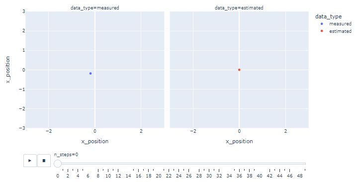
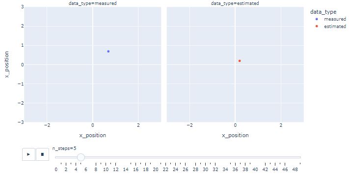
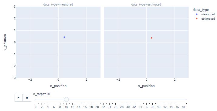


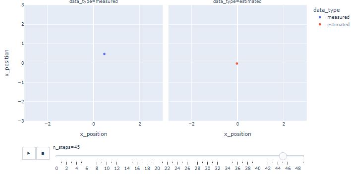

- One can see that KF estimates converge near the actual position as the iterations progress.
- With this basic DP example, we demonstrate how to use KF to process noisy DP data. Similarly, noisy wind, current and acoustic DP data can be filtered before usage.
- Results can be generalized by defining mathematical model of the ship and adding velocity, acceleration, wind and current data to the related KF matrices.
Smoothed Position and Speed Estimates
- Let’s invoke the class KalmanFilter to estimate a sinusoidal trajectory and speed
import numpy as np


class KalmanFilter:
    def __init__(self, x_0: np.ndarray, p: np.ndarray, phi: np.ndarray, gamma: np.ndarray, delta: np.ndarray,
                 cv: np.ndarray,
                 cw: np.ndarray):
        """
        Kalman filter
        :param x_0: Initial state vector
        :param p: Initial covariance matrix on x_0
        :param phi: State transition matrix
        :param gamma: Command model matrix
        :param delta: Sensors model matrix
        :param cv: Variance on step
        :param cw: Variance on sensors
        """
        self._x_hat = x_0
        self._num_states, _ = self._x_hat.shape
        self._p = p
        self._phi = phi
        self._gamma = gamma
        self._delta = delta
        self._cv = cv
        self._cw = cw

    def step(self, u: np.ndarray):
        """
        Step the Kalman filter
        :param u: command vector
        :return: None
        """
        self._x_hat = self._phi @ self._x_hat + self._gamma @ u
        self._p = self._phi @ self._p @ self._phi.T + self._cv

    def update(self, measure):
        """
        Update the Kalman filter with a measure
        :param measure: measurement made
        :return: None
        """
        z_hat = self._delta @ self._x_hat
        r = measure - z_hat
        k = self._p @ self._delta.T @ np.linalg.pinv(self._delta @ self._p @ self._delta.T + self._cw)
        self._x_hat = self._x_hat + k @ r
        self._p = (np.identity(self._num_states) - k @ self._delta) @ self._p

    @property
    def x_hat(self):
        return self._x_hat


if __name__ == '__main__':
    import matplotlib.pyplot as plt

    dt = 1
    x_0 = np.array([[0], [0]])
    p = np.array([[1, 0], [0, 1]]) * 1
    phi = np.array([[1, dt], [0, 1]])
    gamma = np.array([[0.5 * dt ** 2], [dt]])
    delta = np.array([[1, 0]])
    cv = np.array([[0, 0], [0, 0.1]])
    cw = np.array([[35 ** 2]])
    kf = KalmanFilter(x_0, p, phi, gamma, delta, cv, cw)

    true_position = 0
    true_speed = 0
    nb_steps = 200
    time = 0

    true_positions = []
    true_speeds = []
    measurements = []
    estimates = []

    for i in range(nb_steps):
        time += dt
        command = np.array([[0.5 * np.cos(time / (nb_steps * dt / 2) * 2 * np.pi)]])

        # update true localization
        noised_command = command + np.random.randn() * 0.2 * np.abs(np.linalg.norm(command))
        true_position = true_position + true_speed * dt + 0.5 * noised_command * dt ** 2
        true_speed = true_speed + noised_command * dt

        measurement = true_position + np.random.randn() * 25
        kf.step(command)
        kf.update(measurement)

        true_positions.append(true_position)
        true_speeds.append(true_speed)
        measurements.append(measurement)
        estimates.append(kf.x_hat)

    true_positions = np.array(true_positions).squeeze()
    true_speeds = np.array(true_speeds).squeeze()
    measurements = np.array(measurements).squeeze()
    estimates = np.array(estimates).squeeze()


    def moving_average(a, n=3):
        ret = np.cumsum(a, dtype=float)
        ret[n:] = ret[n:] - ret[:-n]
        return ret[n - 1:] / n


    def exponential_average(a, w):
        out = np.zeros_like(a)
        out[0] = a[0]
        for i in range(1, len(a)):
            out[i] = (1 - w) * out[i - 1] + w * a[i]
        return out


    m_average = moving_average(measurements, n=5)
    exp_average = exponential_average(measurements, 0.3)
- Comparison with the true position, measurements vs estimated data by KF and moving/exponential average
   plt.plot(range(nb_steps), true_positions, label='True position')
    plt.scatter(range(nb_steps), measurements, marker='x', label='Measurements')
    plt.plot(range(nb_steps), estimates[:, 0], label='Kalman filter')
    plt.plot(range(len(m_average)), m_average, label='Moving average')
    plt.plot(range(len(exp_average)), exp_average, label='Exponential average')
    plt.title('Position estimate')
    plt.xlabel('Time')
    plt.ylabel('Position')
    plt.legend()
    plt.show()

    plt.plot(range(nb_steps), true_speeds, label='True speed')
    plt.plot(range(nb_steps), estimates[:, 1], label='Kalman filter')
    plt.title('Speed estimate')
    plt.xlabel('Time')
    plt.ylabel('Speed')
    plt.legend()
    plt.show()

Radar EKF Trajectory
- Let’s apply the EKF approach to the noisy radar measurements
import numpy as np
from numpy.linalg import inv
import matplotlib.pyplot as plt

A, Q, R = None, None, None
x, P = None, None
firstRun = True

def Hjacob(xp):
    H = np.zeros([1,3])
    x1 = xp[0]
    x3 = xp[2]
    H[:,0] = x1 / np.sqrt(x1**2 + x3**2)
    H[:,1] = 0
    H[:,2] = x3 / np.sqrt(x1**2 + x3**2)
    return H

def hx(xhat):
    x1 = xhat[0]
    x3 = xhat[2]

    zp = np.sqrt(x1**2 + x3**2)
    return zp


z = radar distance
  = np.sqrt(pos**2 + alt**2) + v
def RadarEKF(z, dt):
    global firstRun
    global A, Q, R, x, P
    if firstRun:
        A = np.eye(3) + dt * np.array([[0,1,0],[0,0,0],[0,0,0]])
        Q = np.array([[0,0,0],[0,0.001,0],[0,0,0.001]])
        R = 10
        x = np.array([0,90,1100]).transpose()
        P = 10 * np.eye(3)
        firstRun = False
    else:
        H = Hjacob(x)
        X_pred = A @ x                          # X_pred : State Variable Prediction
        P_pred = A @ P @ A.T + Q                # Error Covariance Prediction

        K = (P_pred @ H.T) @ inv(H@P_pred@H.T + R) # K : Kalman Gain

        x = X_pred + K@(np.array([z - hx(X_pred)])) # Update State Variable Estimation
        P = P_pred - K@H@P_pred # Update Error Covariance Estimation

    pos = x[0]
    vel = x[1]
    alt = x[2]
    return pos, vel, alt
- Running the test program and plotting the result
# ------ Test program

dt = 0.05
t = np.arange(0, 20, dt)
Nsamples = len(t)
Xsaved = np.zeros([Nsamples,3])
Zsaved = np.zeros([Nsamples,1])
Estimated = np.zeros([Nsamples,1])


pos_pred = None
def GetRadar(dt):
    global pos_pred
    if pos_pred == None:
        pos_pred = 0

    vel = 100 + 5*np.random.randn()
    pos = pos_pred + vel*dt

    alt = 1000 + 10*np.random.randn()
    v = 0 + pos*0.05*np.random.randn()
    r = np.sqrt(pos**2 + alt**2) + v

    pos_pred = pos
    return r


for k in range(Nsamples):
    r = GetRadar(dt)
    print(r)

    pos, vel, alt = RadarEKF(r, dt)

    Xsaved[k] = [pos, vel, alt]
    Zsaved[k] = r
    Estimated[k] = hx([pos, vel, alt])

PosSaved = Xsaved[:,0]
VelSaved = Xsaved[:,1]
AltSaved = Xsaved[:,2]

t = np.arange(0, Nsamples * dt ,dt)

fig = plt.figure()
plt.subplot(313)
plt.plot(t, PosSaved)
plt.xlabel('Time [Sec]')
plt.ylabel('Position [m]')

plt.subplot(311)
plt.plot(t, VelSaved)
plt.xlabel('Time [Sec]')
plt.ylabel('Speed [m/s]')

plt.subplot(312)
plt.plot(t, AltSaved)
plt.xlabel('Time [Sec]')
plt.ylabel('Altitude [m]')

plt.figure()
plt.plot(t, Zsaved, 'r--', label='Measured')
plt.plot(t, Estimated, 'b-', label='Estimated')
plt.xlabel('Time [Sec]')
plt.ylabel('Radar distance [m]')
plt.legend(loc='upper left')

plt.show()
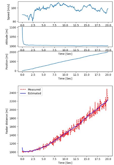
- The EKF is a special KF used when working with nonlinear systems. Since the regular KF can not be applied to nonlinear systems, the EKF was created to solve that problem.
- This example confirms that the EKF does represent the true non-linear system state in the presence of strong measurement noise.
Conclusions
- In this study, the path tracking based on KF and its extensions (like EKF and UKF) is analyzed in terms of the tracking accuracy and precision of hidden variables in the presence of uncertainty.
- This article also presents the comprehensive error analysis of KF-based tracking models for both linear and non-linear noisy measurements.
- As we saw in our scenario testing, KF can be used whenever we need to predict the next state of a system based on some noisy measurements.
- The true and filtered responses of the proposed KF algorithms for object tracking are observed and verified.
- Our simulations demonstrate the excellent robustness and computational efficiency of KF algorithms, making them suitable for real-time deployment.
- Numerical results showed the efficacy of KF. Therefore, this study serves as a hands-on tutorial that helps engineers and data scientists who need a simple, fast, accurate and an easy-to-use implementation of KF for various industry applications.
Explore More
References
- What I Was Missing While Using The Kalman Filter For Object Tracking
- An Easy Explanation of Kalman Filter
- A fast introduction to the tracking and to the Kalman filter
- Kalman-based velocity-free trajectory tracking control of an underactuated aerial vehicle with unknown system dynamics
- Kalman Filter for Moving Object Tracking: Performance Analysis and Filter Design
- Kalman-filter-based Accurate Trajectory Tracking and Fault-Tolerant Control of Quadrotor
- Object Tracking: Kalman Filter with Ease
- Use Kalman Filter for Object Tracking
- Extended Kalman Filter (EKF) With Python Code Example
- A Brief Introduction to Kalman Filters
- Understanding Kalman Filter for Computer Vision


One-Time
Monthly
Yearly
Make a one-time donation
Make a monthly donation
Make a yearly donation
Choose an amount
€5.00
€15.00
€100.00
€5.00
€15.00
€100.00
€5.00
€15.00
€100.00
Or enter a custom amount
€
Your contribution is appreciated.
Your contribution is appreciated.
Your contribution is appreciated.
DonateDonate monthlyDonate yearly
Leave a comment