Oracle Monte Carlo Stock Simulations

import os
os.chdir('YOURPATH')    # Set working directory
os. getcwd()

import datetime as dt
from datetime import datetime as dt
from dateutil.relativedelta import relativedelta
import yfinance as yf  
end = dt.today()
start = dt.today() - relativedelta(years=1)
data = yf.download('ORCL', start, end)
data.tail()

# Distribution parameters
v = 2.91162520
scale = 1.21872294e-02
loc = -8.13209384e-05
# importing the datetime library to generate dates for the future

from datetime import datetime, timedelta
from scipy import stats

# the simulations' starting price
initial_price = data['Close'].iloc[-1]
# number of simulation days
N_steps = 14
# number of scenarios in simulation
N_sims = 1000
# here we sample the distribution for 14x50000 future returns
rets_t= stats.t.rvs(df= v,loc = loc, scale =scale, size = (N_steps, N_sims))
# here we calculate the price at each timestep from the generated log returns
sim = (np.exp(rets_t.cumsum(axis = 1)))
# we save the results in a dataframe and put them on equal footing
results = pd.DataFrame(np.array(sim).reshape(N_sims, N_steps).T)
results = results.divide(results.iloc[0])*initial_price

time = pd.date_range(start = data.index[-1],
                     end = data.index[-1] + timedelta(days = N_steps - 1))
# lets look at the final price 
final_price_t = results.iloc[-1] 

plt.figure(figsize=(10,6))
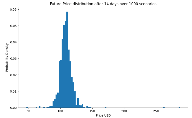
plt.hist(final_price_t[final_price_t < 5*initial_price], density = True, bins = 100)
plt.title(f'Future Price distribution after {N_steps} days over {N_sims} scenarios')
plt.xlabel('Price USD')
plt.ylabel('Probability Density')

print (time)

DatetimeIndex(['2023-10-19', '2023-10-20', '2023-10-21', '2023-10-22',
               '2023-10-23', '2023-10-24', '2023-10-25', '2023-10-26',
               '2023-10-27', '2023-10-28', '2023-10-29', '2023-10-30',
               '2023-10-31', '2023-11-01'],
              dtype='datetime64[ns]', freq='D')

plt.figure(figsize=(18,15))
SMALL_SIZE = 20
MEDIUM_SIZE = 20
BIGGER_SIZE = 20
plt.rc('font', size=SMALL_SIZE)          # controls default text sizes
plt.rc('axes', titlesize=SMALL_SIZE)     # fontsize of the axes title
plt.rc('axes', labelsize=MEDIUM_SIZE)    # fontsize of the x and y labels
plt.rc('xtick', labelsize=18)    # fontsize of the tick labels
plt.rc('ytick', labelsize=SMALL_SIZE)    # fontsize of the tick labels
plt.rc('legend', fontsize=SMALL_SIZE)    # legend fontsize
plt.rc('figure', titlesize=BIGGER_SIZE)  # fontsize of the figure title
plt.xticks(rotation=45, ha='right')
plt.plot(time,results)
plt.xlabel('Date')
plt.ylabel('Price USD')
plt.title('Oracle Price Monte Carlo Simulation')
plt.ylim(top=200)