
- Machine learning (ML) is an important decision support tool for crop yield prediction, including supporting decisions on what crops to grow and what to do during the growing season of the crops.
- Following recent research studies, this case example investigates whether coupling crop modeling, exploratory data analysis (EDA), ML yield prediction, recommendation, and multi-label classification algorithms yield competitive results with respect to the crop growth model. The main objectives are to explore whether a hybrid approach would result in better predictions, investigate which combinations of hybrid models provide the most accurate predictions, and determine the features from the crop modeling that are most effective to be integrated with ML for smart farming.
Table of Contents
- CatBoost/SHAP: Indian Crop Yield
- ML-Powered Indian Agriculture
- Global Crop Yield Prediction
- Crop Recommendation
- Effects of Climate Changes
- Summary
- Explore More
CatBoost/SHAP: Indian Crop Yield
- We begin our study with the Agricultural crop yield prediction in Indian states using the CatBoost & SHAP algorithms in Python.
- Agricultural Crop Yield in Indian States Dataset (DAT1):
This dataset encompasses agricultural data for multiple crops cultivated across various states in India from the year 1997 till 2020. The dataset provides crucial features related to crop yield prediction, including crop types, crop years, cropping seasons, states, areas under cultivation, production quantities, annual rainfall, fertilizer usage, pesticide usage, and calculated yields.
- Data Columns Description:
- Crop: The name of the crop cultivated.
- Crop_Year: The year in which the crop was grown.
- Season: The specific cropping season (e.g., Kharif, Rabi, Whole Year).
- State: The Indian state where the crop was cultivated.
- Area: The total land area (in hectares) under cultivation for the specific crop.
- Production: The quantity of crop production (in metric tons).
- Annual_Rainfall: The annual rainfall received in the crop-growing region (in mm).
- Fertilizer: The total amount of fertilizer used for the crop (in kilograms).
- Pesticide: The total amount of pesticide used for the crop (in kilograms).
- Yield: The calculated crop yield (production per unit area).
- Set the working directory YOURPATH
import os
os.chdir('YOURPATH')
os. getcwd()
- Import and install the key libraries
!pip install feature_engine
# import libraries
import numpy as np # linear algebra
import pandas as pd # data processing, CSV file I/O (e.g. pd.read_csv)

import warnings
warnings.filterwarnings("ignore")

import shap
import matplotlib.pyplot as plt
from catboost import Pool, CatBoostRegressor
from sklearn.metrics import mean_squared_error
from sklearn.model_selection import train_test_split
from feature_engine.encoding import RareLabelEncoder
from sklearn.feature_extraction.text import CountVectorizer
import ast
- Read the input Kaggle dataset DAT1
df = pd.read_csv("crop_yield.csv").drop_duplicates()
print(df.shape)
df.sample(5).T
(19689, 10)

df.info()
<class 'pandas.core.frame.DataFrame'>
Int64Index: 19689 entries, 0 to 19688
Data columns (total 10 columns):
 #   Column           Non-Null Count  Dtype
---  ------           --------------  -----
 0   Crop             19689 non-null  object
 1   Crop_Year        19689 non-null  int64
 2   Season           19689 non-null  object
 3   State            19689 non-null  object
 4   Area             19689 non-null  float64
 5   Production       19689 non-null  int64
 6   Annual_Rainfall  19689 non-null  float64
 7   Fertilizer       19689 non-null  float64
 8   Pesticide        19689 non-null  float64
 9   Yield            19689 non-null  float64
dtypes: float64(5), int64(2), object(3)
memory usage: 1.7+ MB
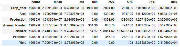
df.describe().T
- EDA via SweetViz
import sweetviz as sv
import pandas as pd
# Create an analysis report for the data
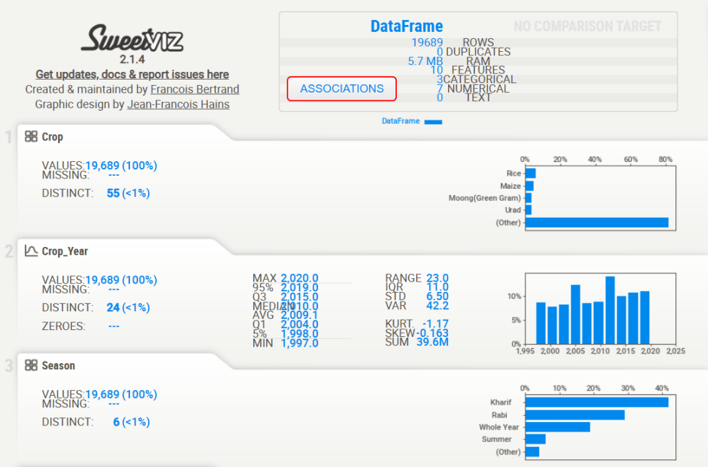
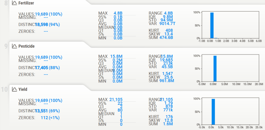
report = sv.analyze(df)
# Display the report
report.show_html()
Report SWEETVIZ_REPORT.html was generated! NOTEBOOK/COLAB USERS: the web browser MAY not pop up, regardless, the report IS saved in your notebook/colab files.

SweetViz associations:
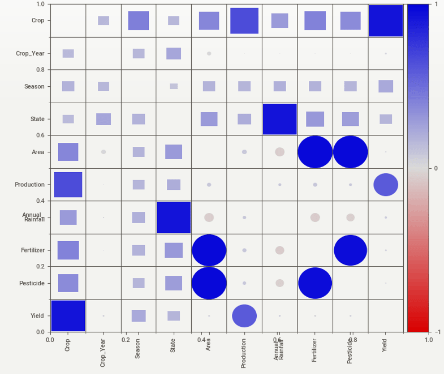
Here, Squares are categorical associations (uncertainty coefficient & correlation ratio) from 0 to 1. The uncertainty coefficient is asymmetrical (i.e. ROW LABEL values indicate how much they PROVIDE INFORMATION to each LABEL at the TOP). Circles are the symmetrical numerical correlations (Pearson’s) from -1 to 1. The trivial diagonal is intentionally left blank for clarity.
- Data preparation
# select records with non-zero yield
df = df[df['Yield']>0]
# select main label
main_label = 'log10_yield'
df[main_label] = df['Yield'].apply(lambda x: np.log10(x))
# divide fertilizer and pesticide by area (in kg/hectare) and annual rainfall (in mm), log10-transform and group into larger bins
for col in ['Fertilizer', 'Pesticide']:
    df[f'log10_{col}_Area'] = (df[col]/df['Area']).apply(lambda x: 1/10*round(10*np.log10(x)))
df['log10_Annual_Rainfall'] = df['Annual_Rainfall'].apply(lambda x: 1/10*round(10*np.log10(x)))
# set up the rare label encoder limiting number of categories to max_n_categories
for col in ['Crop', 'Season', 'State']:
    encoder = RareLabelEncoder(n_categories=1, max_n_categories=50, replace_with='Other', tol=25/df.shape[0])
    df[col] = encoder.fit_transform(df[[col]])
# drop unused columns
cols2drop = ['Production', 'Yield', 'Fertilizer', 'Pesticide', 'Area', 'Annual_Rainfall']
df = df.drop(cols2drop, axis=1)
- Train/test data splitting as 70:30
y = df[main_label].values.reshape(-1,)
X = df.drop([main_label], axis=1)
cat_cols = df.select_dtypes(include=['object']).columns
cat_cols_idx = [list(X.columns).index(c) for c in cat_cols]
X_train,X_test,y_train,y_test = train_test_split(X, y, test_size=0.3, random_state=0)
X_train.shape, X_test.shape, y_train.shape, y_test.shape
- Model training, validation and prediction
# initialize Pool
train_pool = Pool(X_train,
                  y_train,
                  cat_features=cat_cols_idx)
test_pool = Pool(X_test,
                 y_test,
                 cat_features=cat_cols_idx)
# specify the training parameters
model = CatBoostRegressor(iterations=1000,
                          depth=5,
                          verbose=0,
                          learning_rate=0.15,
                          loss_function='RMSE')
# train the model
model.fit(train_pool)
# make the prediction using the resulting model
y_train_pred = model.predict(train_pool)
y_test_pred = model.predict(test_pool)

rmse_train = mean_squared_error(y_train, y_train_pred, squared=False)
rmse_test = mean_squared_error(y_test, y_test_pred, squared=False)
print(f"RMSE score for train {round(rmse_train,3)} dex, and for test {round(rmse_test,3)} dex")
RMSE score for train 0.152 dex, and for test 0.168 dex
# Baseline scores (assuming the same prediction for all data samples)
rmse_bs_train = mean_squared_error(y_train, [np.mean(y_train)]*len(y_train), squared=False)
rmse_bs_test = mean_squared_error(y_test, [np.mean(y_train)]*len(y_test), squared=False)
print(f"RMSE baseline score for train {round(rmse_bs_train,3)} dex, and for test {round(rmse_bs_test,3)} dex")
RMSE baseline score for train 0.648 dex, and for test 0.662 dex
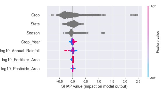
- SHAP initialization and summary value plot
shap.initjs()
ex = shap.TreeExplainer(model)
shap_values = ex.shap_values(X_test)
shap.summary_plot(shap_values, X_test)
- Expected vs actual log10 yield values
expected_values = ex.expected_value
print(f"Average predicted log10 yield is {round(expected_values,3)} dex")
print(f"Average actual log10 yield is {round(np.mean(y_test),3)} dex")
Average predicted log10 yield is 0.166 dex
Average actual log10 yield is 0.166 dex
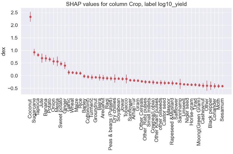
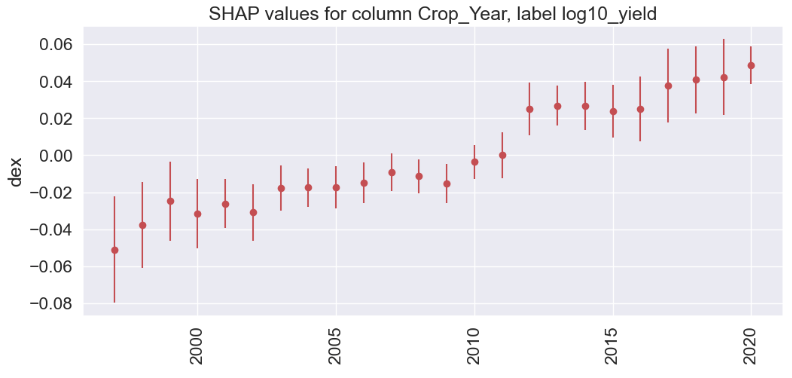
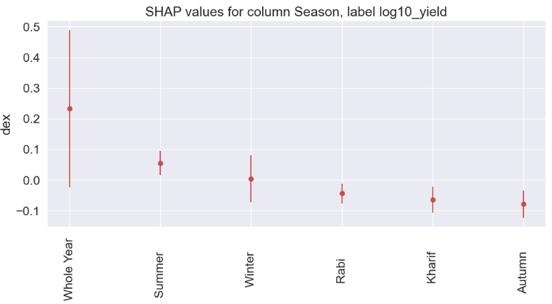
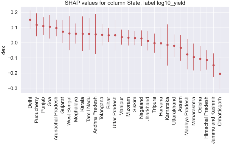
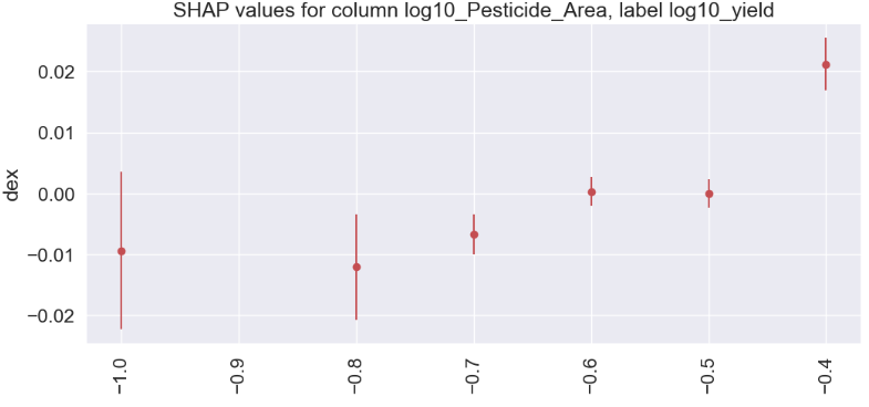
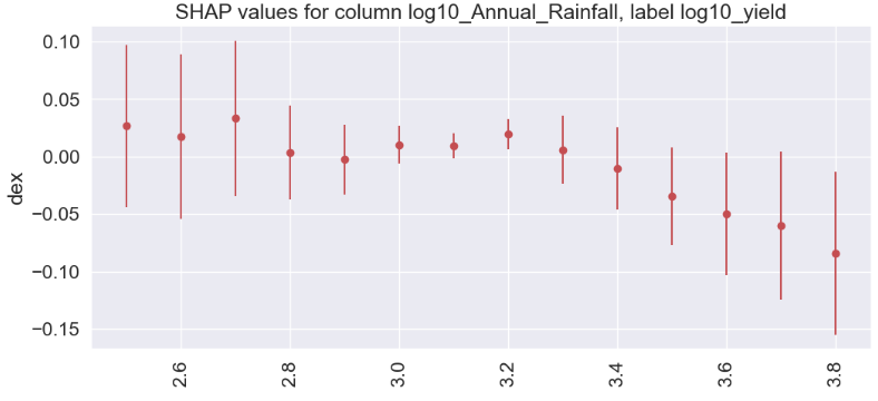
- SHAP values for log10 columns vs log10 yield
def show_shap(col, shap_values=shap_values, label=main_label, X_test=X_test, ylabel='dex'):
    df_infl = X_test.copy()
    df_infl['shap_'] = shap_values[:,df_infl.columns.tolist().index(col)]
    gain = round(df_infl.groupby(col).mean()['shap_'],4)
    gain_std = round(df_infl.groupby(col).std()['shap_'],4)
    cnt = df_infl.groupby(col).count()['shap_']
    dd_dict = {'col': list(gain.index), 'gain': list(gain.values), 'gain_std': list(gain_std.values), 'count': cnt}
    df_res = pd.DataFrame.from_dict(dd_dict).sort_values('gain', ascending=False).set_index('col')
    plt.figure(figsize=(12,5))
    plt.errorbar(df_res.index, df_res['gain'], yerr=df_res['gain_std'], fmt="o", color="r")
    plt.title(f'SHAP values for column {col}, label {label}')
    plt.ylabel(ylabel)
    plt.tick_params(axis="x", rotation=90)
    plt.show();
    print(df_res)
    return

for col in X_test.columns:
    print()
    print(col)
    print()
    show_shap(col, shap_values, label=main_label, X_test=X_test)
Crop
                         gain  gain_std  count
col
Coconut                2.3294    0.1996     55
Sugarcane              0.9245    0.1310    185
Tapioca                0.8204    0.0767     61
Jute                   0.6929    0.1759     46
Banana                 0.6839    0.1331     68
Potato                 0.6438    0.0909    178
Onion                  0.5671    0.1460    143
Mesta                  0.5604    0.1945     49
Sweet potato           0.4691    0.0912     72
Ginger                 0.4002    0.1407     97
Garlic                 0.1264    0.0891     76
Wheat                  0.1169    0.0587    153
Maize                  0.1059    0.0672    311
Rice                   0.0945    0.0729    384
Barley                -0.0268    0.0749     82
Cotton(lint)          -0.0511    0.0750    146
Turmeric              -0.0662    0.1038    105
Groundnut             -0.0683    0.0526    217
Bajra                 -0.0751    0.1232    170
Arecanut              -0.0916    0.1117     42
Ragi                  -0.1053    0.0804    150
Peas & beans (Pulses) -0.1158    0.0847    115
Dry chillies          -0.1196    0.1651    113
Soyabean              -0.1201    0.0592    121
Jowar                 -0.1299    0.0718    136
Tobacco               -0.1349    0.1737     94
Sunflower             -0.1842    0.0569    131
Arhar/Tur             -0.1927    0.0588    158
Gram                  -0.2001    0.0586    141
Other Cereals         -0.2332    0.0541     56
Other  Rabi pulses    -0.2515    0.0787    102
Small millets         -0.2562    0.0500    144
Cowpea(Lobia)         -0.2679    0.0893     36
Other Kharif pulses   -0.2808    0.0557    112
other oilseeds        -0.2836    0.1094     42
Castor seed           -0.2889    0.0858     80
Masoor                -0.2919    0.0530     90
Rapeseed &Mustard     -0.2971    0.0954    146
Safflower             -0.3099    0.0389     56
Sannhamp              -0.3295    0.2001     43
Linseed               -0.3501    0.0361     86
Niger seed            -0.3542    0.0463     59
Horse-gram            -0.3634    0.0543    116
Urad                  -0.3636    0.0596    248
Moong(Green Gram)     -0.3797    0.0658    203
Cashewnut             -0.3963    0.1056     30
Other                 -0.4002    0.2008     79
Black pepper          -0.4069    0.1651     37
Coriander             -0.4146    0.1051     57
Moth                  -0.4195    0.0815     32
Sesamum               -0.4215    0.0527    221
Crop_Year
        gain  gain_std  count
col
2020  0.0488    0.0102     15
2019  0.0422    0.0205    321
2018  0.0407    0.0180    319
2017  0.0377    0.0200    309
2013  0.0268    0.0109    289
2014  0.0267    0.0131    264
2016  0.0252    0.0175    316
2012  0.0250    0.0142    262
2015  0.0238    0.0144    297
2011 -0.0000    0.0125    288
2010 -0.0036    0.0092    269
2007 -0.0092    0.0103    221
2008 -0.0114    0.0091    259
2006 -0.0148    0.0110    262
2009 -0.0153    0.0107    245
2005 -0.0173    0.0115    233
2004 -0.0175    0.0105    232
2003 -0.0177    0.0122    260
1999 -0.0248    0.0214    203
2001 -0.0261    0.0134    236
2002 -0.0308    0.0153    237
2000 -0.0316    0.0187    239
1998 -0.0376    0.0233    177
1997 -0.0511    0.0287    121
Season
               gain  gain_std  count
col
Whole Year   0.2325    0.2568   1078
Summer       0.0551    0.0395    369
Winter       0.0032    0.0770    124
Rabi        -0.0439    0.0326   1645
Kharif      -0.0642    0.0427   2542
Autumn      -0.0786    0.0443    116
State
                      gain  gain_std  count
col
Delhi              0.1506    0.0605     54
Puducherry         0.1170    0.0756    208
Punjab             0.1086    0.0567    129
Goa                0.1046    0.0778     68
Arunachal Pradesh  0.0961    0.0548     82
Gujarat            0.0729    0.0755    256
West Bengal        0.0610    0.1118    354
Meghalaya          0.0595    0.0662    175
Kerala             0.0579    0.1140    154
Tamil Nadu         0.0567    0.1042    237
Andhra Pradesh     0.0547    0.1312    382
Telangana          0.0514    0.0705    115
Bihar              0.0492    0.0456    263
Uttar Pradesh      0.0478    0.1003    220
Manipur            0.0360    0.0498    123
Mizoram            0.0317    0.0508    135
Sikkim             0.0291    0.0479     85
Nagaland           0.0282    0.0517    224
Jharkhand          0.0108    0.0624     82
Tripura           -0.0036    0.0627    144
Haryana           -0.0049    0.1052    163
Karnataka         -0.0156    0.1353    415
Uttarakhand       -0.0206    0.0734    231
Assam             -0.0346    0.0840    214
Madhya Pradesh    -0.0773    0.1000    249
Maharashtra       -0.0953    0.0888    228
Odisha            -0.1070    0.0836    238
Himachal Pradesh  -0.1144    0.0643    181
Jammu and Kashmir -0.1489    0.0770    187
Chhattisgarh      -0.2043    0.1029    278
log10_Pesticide_Area
        gain  gain_std  count
col
-0.4  0.0212    0.0043    645
-0.6  0.0003    0.0024   1733
-0.5  0.0000    0.0023   2044
-0.7 -0.0067    0.0033    727
-1.0 -0.0094    0.0129    259
-0.8 -0.0121    0.0087    466
- log10_Annual_Rainfall
       gain  gain_std  count
col
2.7  0.0332    0.0678    143
2.5  0.0267    0.0705     72
3.2  0.0196    0.0134    978
2.6  0.0174    0.0719     88
3.0  0.0104    0.0166   1175
3.1  0.0093    0.0111   1334
3.3  0.0058    0.0296    464
2.8  0.0036    0.0407    293
2.9 -0.0027    0.0302    554
3.4 -0.0105    0.0359    394
3.5 -0.0346    0.0426    241
3.6 -0.0499    0.0532     87
3.7 -0.0599    0.0642     23
3.8 -0.0840    0.0708     28
ML-Powered Indian Agriculture
- In this section, we will focus on the Indian Agricultural Crop Yield Predictions using supervised ML algorithms and the aforementioned input dataset DAT1. Our objective is to overcome observed shortcomings of basic linear regression applied to DAT1.
- Basic imports and load input dataset DAT1
# Importing Libraries
import numpy as np
import pandas as pd
import matplotlib.pyplot as plt
import seaborn as sns
import plotly.express as px

import warnings
warnings.filterwarnings('ignore')
# Loading the dataset
df = pd.read_csv('crop_yield.csv')
- Exploratory Data Analysis (EDA)
Measure of Yield over the year < 2020
df_year = df[df['Crop_Year']!=2020]
year_yield = df_year.groupby('Crop_Year').sum()


plt.figure(figsize = (12,5))
plt.plot(year_yield.index, year_yield['Yield'],color='blue', linestyle='dashed', marker='o',
        markersize=12, markerfacecolor='yellow')
plt.xlabel('Year')
plt.ylabel('Yield')
plt.title('Measure of Yield over the year')
plt.show()

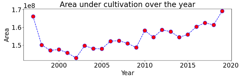
Area under cultivation over the year
plt.figure(figsize = (12,3))
plt.plot(year_yield.index, year_yield['Area'],color='blue', linestyle='dashed', marker='o',
        markersize=12, markerfacecolor='red')
plt.xlabel('Year')
plt.ylabel('Area')
plt.title('Area under cultivation over the year')
plt.show()
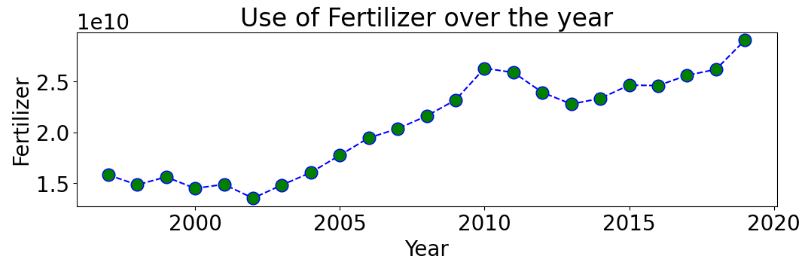
Use of Fertilizer over the year
plt.figure(figsize = (12,3))
plt.plot(year_yield.index, year_yield['Fertilizer'],color='blue', linestyle='dashed', marker='o',
        markersize=12, markerfacecolor='green')
plt.xlabel('Year')
plt.ylabel('Fertilizer')
plt.title('Use of Fertilizer over the year')
plt.show()
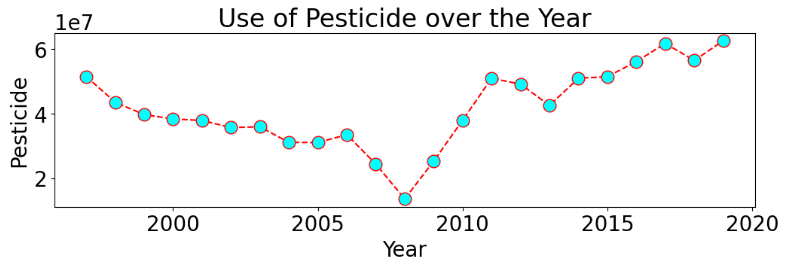
Use of Pesticide over the Year
plt.figure(figsize = (12,3))
plt.plot(year_yield.index, year_yield['Pesticide'],color='red', linestyle='dashed', marker='o',
        markersize=12, markerfacecolor='cyan')
plt.xlabel('Year')
plt.ylabel('Pesticide')
plt.title('Use of Pesticide over the Year')
plt.show()
Yield vs Region/State
df_state = df.groupby('State').sum()
df_state.sort_values(by = 'Yield', inplace=True, ascending = False)
df_state['Region'] = ['States' for i in range(len(df_state))]

fig = px.bar(df_state, x='Region', y = 'Yield', color=df_state.index, hover_data=['Yield'])
fig.show()

Bar Plot Annual Rainfall vs State
plt.figure(figsize = (15,8))
sns.barplot(x = df_state.index, y=df_state['Annual_Rainfall'], palette = 'gnuplot')
plt.xticks(rotation = 90)
plt.savefig('annualrainfallstate.png')

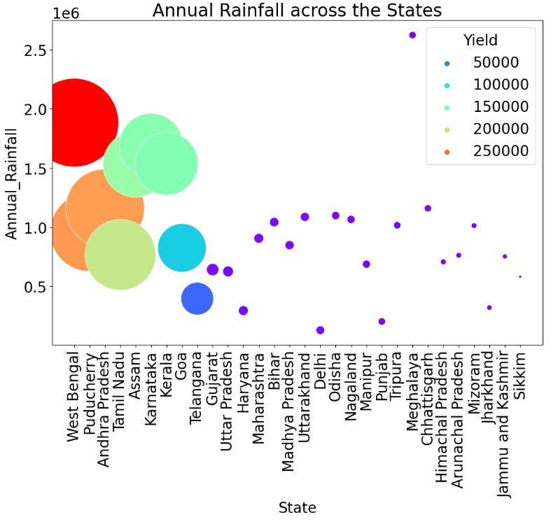
Bubble Plot Annual Rainfall and Yield across the States
plt.figure(figsize=(12,8))
sns.scatterplot(x=df_state.index, y = df_state['Annual_Rainfall'], palette='rainbow', hue = df_state['Yield'],s=df_state['Yield']/20)
plt.xticks(rotation=90)
plt.title('Annual Rainfall across the States')
plt.show()
Bubble Plot Fertilizer and Yield vs State
plt.figure(figsize=(12,8))
sns.scatterplot(x=df_state.index, y=df_state['Fertilizer'], palette='spring', hue = df_state['Yield'],s=df_state['Yield']/20)
plt.xticks(rotation=90)
plt.title('Use of Fertilizer in Different States')
plt.show()

Plotly Bar Plot Area vs Season
df_Seas = df[df['Season']!='Whole Year ']

df_season = df_Seas.groupby('Season').sum()
fig = px.bar(df_season, y = 'Area', color=df_season.index, hover_data=['Area'],text = 'Area')
fig.update_layout(
    font=dict(
        family="Courier New, monospace",
        size=18,  # Set the font size here
        color="RebeccaPurple"
    )
)
fig.show()

Plotly Pie Chart Yield vs Season
fig = px.sunburst(df_season, path=[df_season.index, 'Yield'], values='Yield',
                  color=df_season.index, hover_data=['Yield'])
fig.update_layout(
    font=dict(
        family="Courier New, monospace",
        size=18,  # Set the font size here
        color="RebeccaPurple"
    ))
fig.show()

States and Crops where Yield=0
df_yz = df[df['Yield']==0]
plt.figure(figsize = (25,15))
sns.catplot(y="State", x="Crop",data=df_yz, aspect = 3, palette ='inferno')
plt.xticks(rotation=90)
plt.title('States and Crops where Yield=0')
plt.show()

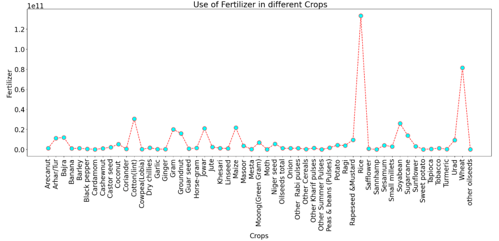
Use of Fertilizer in different Crops for States with Yield>0
df_ynz = df[df['Yield']>0]  # where yield is more than zero
df_crop = df_ynz.groupby('Crop').sum()
plt.figure(figsize = (25,8))
plt.plot(df_crop.index, df_crop['Fertilizer'],color='red', linestyle='dashed', marker='o',
        markersize=12, markerfacecolor='cyan')
plt.rcParams.update({'font.size': 20})
plt.xlabel('Crops')
plt.ylabel('Fertilizer')
plt.title(' Use of Fertilizer in different Crops')
plt.xticks(rotation=90)
plt.show()
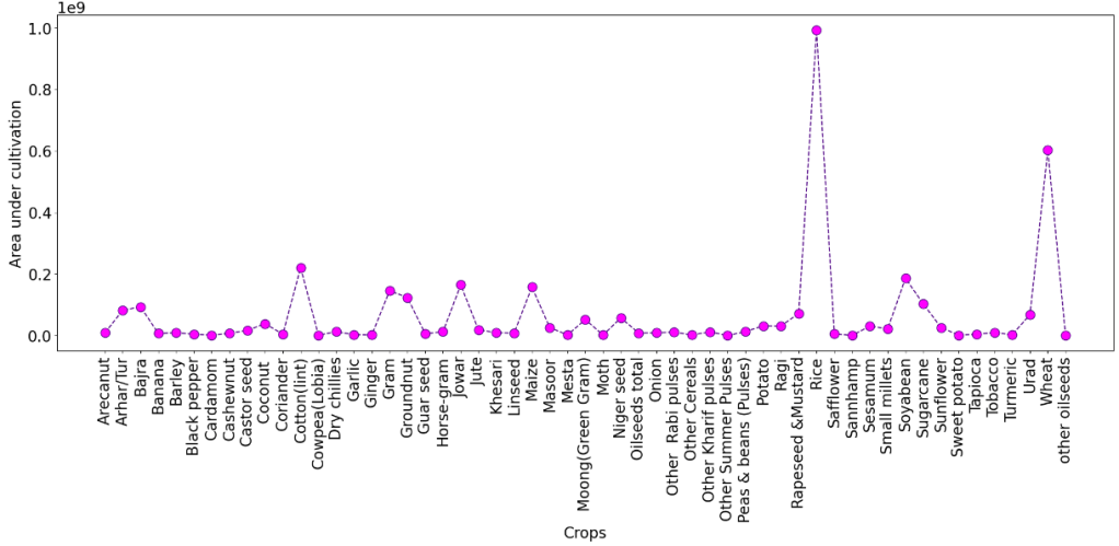
Area under Cultivation in different Crops for States with Yield>0
plt.figure(figsize = (25,8))
plt.rcParams.update({'font.size': 20})
plt.plot(df_crop.index, df_crop['Area'],color='indigo', linestyle='dashed', marker='o',
        markersize=12, markerfacecolor='fuchsia')
plt.xlabel('Crops')
plt.ylabel('Area under cultivation')
plt.xticks(rotation=90)
plt.show()
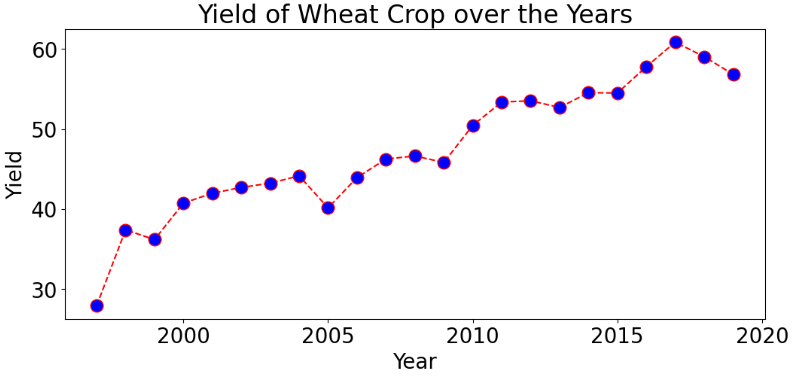
Yield of Wheat Crop over the Years
df_wheat = df[df['Crop']=='Wheat']
df_wheat.reset_index(drop=True,inplace=True)
df_wheat1 = df_wheat[df_wheat['Crop_Year']!=2020]
df_wheat_year = df_wheat1.groupby('Crop_Year').sum()
plt.figure(figsize = (12,5))
plt.plot(df_wheat_year.index, df_wheat_year['Yield'],color='red', linestyle='dashed', marker='o',
        markersize=12, markerfacecolor='blue')
plt.xlabel('Year')
plt.ylabel('Yield')
plt.title('Yield of Wheat Crop over the Years')
plt.show()
Empirical Probability Analysis, Train/Test Split and Power Transformation
df1 = df.copy()
df1 = df1.drop(['Crop_Year','Pesticide'], axis = 1)
category_columns = df1.select_dtypes(include = ['object']).columns
df1 = pd.get_dummies(df1, columns = category_columns, drop_first=True)
x = df1.drop(['Yield'], axis = 1)
y = df1[['Yield']]
#split the data into training and test set as 70:30 %
from sklearn.model_selection import train_test_split
x_train, x_test, y_train,y_test = train_test_split(x, y, test_size = 0.3, random_state = 42)
from sklearn.preprocessing import PowerTransformer
pt = PowerTransformer(method='yeo-johnson')

x_train_transform1 = pt.fit_transform(x_train)
x_test_transform1 = pt.fit_transform(x_test)
df_trans = pd.DataFrame(x_train_transform1, columns=x_train.columns)
Histograms of transformed data: Area, Production, Annual Rainfall, and Fertilizer
plt.figure(figsize=(15,20))
plt.subplot(4,2,1)
sns.distplot(df_trans['Area'],bins = 20,color = 'red')
plt.subplot(4,2,2)
sns.distplot(df_trans['Production'],bins = 10,color = 'green')
plt.subplot(4,2,3)
sns.distplot(df_trans['Annual_Rainfall'],bins = 10,color = 'fuchsia')
plt.subplot(4,2,4)
sns.distplot(df_trans['Fertilizer'],bins = 10, color = 'indigo')

plt.show()

Q-Q probability plots of transformed data: Area, Production, Annual Rainfall, and Fertilizer
plt.figure(figsize=(15,40))
plt.subplot(4,2,1)
stats.probplot(df_trans['Area'], dist = 'norm', plot = plt)
plt.subplot(4,2,2)
stats.probplot(df_trans['Production'], dist = 'norm', plot = plt)
plt.subplot(4,2,3)
stats.probplot(df_trans['Annual_Rainfall'], dist = 'norm', plot = plt)
plt.subplot(4,2,4)
stats.probplot(df_trans['Fertilizer'], dist = 'norm', plot = plt)

plt.show()
Q-Q Plot Area Q-Q Plot Production
Q-Q Plot Annual Rainfall Q-Q Plot Fertilizer
- Linear Regression before Transform
from sklearn.linear_model import LinearRegression
from sklearn.metrics import r2_score

lr = LinearRegression()
lr.fit(x_train,y_train)

y_pred_train = lr.predict(x_train)
print("Training Accuracy : ",r2_score(y_train,y_pred_train))

y_pred_test = lr.predict(x_test)
print("Test Accuracy : ",r2_score(y_test,y_pred_test))
Training Accuracy :  0.8626702222423179
Test Accuracy :  0.7954868193972229
# Initialization to store accuracy value
train_accu = []
test_accu = []
- Linear Regression after Transform
lr.fit(x_train_transform1, y_train)

y_pred_train_ = lr.predict(x_train_transform1)
y_pred_test_ = lr.predict(x_test_transform1)

print("Training Accuracy : ",r2_score(y_train, y_pred_train_))
print()
print("Test Accuracy : ",r2_score(y_test, y_pred_test_))

train_accu.append(r2_score(y_train,y_pred_train_))
test_accu.append(r2_score(y_test,y_pred_test_))
Training Accuracy :  0.8660561096838644
Test Accuracy :  0.8089635049182979
- Variance Inflation Factor (VIF) of Transformed Data
x1 = df_trans.copy()
from statsmodels.stats.outliers_influence import variance_inflation_factor

variable = x1

vif = pd.DataFrame()

vif['Variance Inflation Factor'] = [variance_inflation_factor(variable, i)
                                    for i in range(variable.shape[1])]

vif['Features'] = x1.columns
x2 = x1.copy()
x2.drop(['Area'], axis = 1, inplace=True)
variable = x2

vif = pd.DataFrame()

vif['Variance Inflation Factor'] = [variance_inflation_factor(variable, i)
                                    for i in range(variable.shape[1])]

vif['Features'] = x2.columns
print (vif)
Variance Inflation Factor             Features
0                   19.613495           Production
1                    6.502925      Annual_Rainfall
2                   18.511399           Fertilizer
3                    4.398463       Crop_Arhar/Tur
4                    4.615635           Crop_Bajra
..                        ...                  ...
86                   1.327546      State_Telangana
87                   1.899844        State_Tripura
88                   1.737332  State_Uttar Pradesh
89                   1.901585    State_Uttarakhand
90                   2.399254    State_West Bengal

[91 rows x 2 columns]
x2.drop(['Production'], axis = 1, inplace=True)
variable = x2

vif = pd.DataFrame()

vif['Variance Inflation Factor'] = [variance_inflation_factor(variable, i)
                                    for i in range(variable.shape[1])]

vif['Features'] = x2.columns
print (vif)
Variance Inflation Factor             Features
0                    6.502762      Annual_Rainfall
1                    2.228737           Fertilizer
2                    4.391123       Crop_Arhar/Tur
3                    4.615516           Crop_Bajra
4                    2.518605          Crop_Banana
..                        ...                  ...
85                   1.325111      State_Telangana
86                   1.895037        State_Tripura
87                   1.737068  State_Uttar Pradesh
88                   1.899269    State_Uttarakhand
89                   2.387405    State_West Bengal

[90 rows x 2 columns]
- Linear Regression after Applying VIF
x_test1 = pd.DataFrame(x_test_transform1, columns=x_test.columns)
x_test1.drop(['Area','Production'], axis = 1, inplace = True)
# After applying vif
lr.fit(x2, y_train)

y_pred_train_ = lr.predict(x2)
y_pred_test_ = lr.predict(x_test1)

print("Training Accuracy : ",r2_score(y_train, y_pred_train_))
print()
print("Test Accuracy : ",r2_score(y_test, y_pred_test_))

train_accu.append(r2_score(y_train,y_pred_train_))
test_accu.append(r2_score(y_test,y_pred_test_))
Training Accuracy :  0.8612782567666339
Test Accuracy :  0.7993727827493086
- Random Forest Regressor of Transformed Data
from sklearn.ensemble import RandomForestRegressor
regr = RandomForestRegressor()

regr.fit(x_train_transform1, y_train)

y_pred_train_regr= regr.predict(x_train_transform1)
y_pred_test_regr = regr.predict(x_test_transform1)

print("Training Accuracy : ",r2_score(y_train, y_pred_train_regr))
print("Test Accuracy : ",r2_score(y_test, y_pred_test_regr))

train_accu.append(r2_score(y_train,y_pred_train_regr))
test_accu.append(r2_score(y_test,y_pred_test_regr))
Training Accuracy :  0.9976015686329384
Test Accuracy :  0.9453495882397677
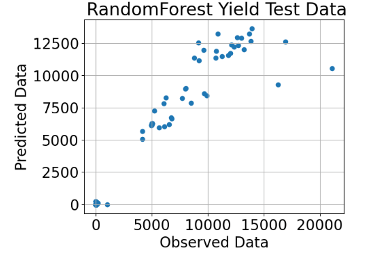
- Random Forest Yield Test Predicted/Observed Transformed Data
plt.scatter(y_test,y_pred_test_regr)

plt.title(" RandomForest Yield Test Data")
plt.xlabel("Observed Data")
plt.ylabel("Predicted Data")
plt.grid()
plt.show()
- Random Forest Regressor of Transformed Data after applying VIF
from sklearn.ensemble import RandomForestRegressor
regr = RandomForestRegressor()


regr.fit(x2, y_train)

y_pred_train_regr= regr.predict(x2)
y_pred_test_regr = regr.predict(x_test1)

print("Training Accuracy : ",r2_score(y_train, y_pred_train_regr))
print("Test Accuracy : ",r2_score(y_test, y_pred_test_regr))

train_accu.append(r2_score(y_train,y_pred_train_regr))
test_accu.append(r2_score(y_test,y_pred_test_regr))
Training Accuracy :  0.9968700195835773
Test Accuracy :  0.9512089658064634
- Random Forest Yield Test Predicted/Observed Transformed Data after applying VIF
plt.scatter(y_test,y_pred_test_regr)
plt.title(" RandomForest Yield Test Data")
plt.xlabel("Observed Data")
plt.ylabel("Predicted Data")
plt.grid()
plt.show()

- Let’s check the accuracy of various regression models
Linear Regression
from sklearn.linear_model import LinearRegression
regr = LinearRegression()
regr.fit(x_train_transform1, y_train)

y_pred_train_regr= regr.predict(x_train_transform1)
y_pred_test_regr = regr.predict(x_test_transform1)

print("Training Accuracy : ",r2_score(y_train, y_pred_train_regr))
print("Test Accuracy : ",r2_score(y_test, y_pred_test_regr))

train_accu.append(r2_score(y_train,y_pred_train_regr))
test_accu.append(r2_score(y_test,y_pred_test_regr))
Training Accuracy :  0.8660561096838644
Test Accuracy :  0.8089635049182979
Ada Boost Regressor
from sklearn.ensemble import AdaBoostRegressor
regr = AdaBoostRegressor()
regr.fit(x_train_transform1, y_train)

y_pred_train_regr= regr.predict(x_train_transform1)
y_pred_test_regr = regr.predict(x_test_transform1)

print("Training Accuracy : ",r2_score(y_train, y_pred_train_regr))
print("Test Accuracy : ",r2_score(y_test, y_pred_test_regr))

train_accu.append(r2_score(y_train,y_pred_train_regr))
test_accu.append(r2_score(y_test,y_pred_test_regr))
Training Accuracy :  0.9753826862500993
Test Accuracy :  0.9432430977757433
Decision Tree Regressor
from sklearn.tree import DecisionTreeRegressor
regr = DecisionTreeRegressor()
regr.fit(x_train_transform1, y_train)

y_pred_train_regr= regr.predict(x_train_transform1)
y_pred_test_regr = regr.predict(x_test_transform1)

print("Training Accuracy : ",r2_score(y_train, y_pred_train_regr))
print("Test Accuracy : ",r2_score(y_test, y_pred_test_regr))

train_accu.append(r2_score(y_train,y_pred_train_regr))
test_accu.append(r2_score(y_test,y_pred_test_regr))
Training Accuracy :  1.0
Test Accuracy :  0.953298449231916
Extra Trees Regressor
from sklearn.ensemble import ExtraTreesRegressor
regr = ExtraTreesRegressor()
regr.fit(x_train_transform1, y_train)

y_pred_train_regr= regr.predict(x_train_transform1)
y_pred_test_regr = regr.predict(x_test_transform1)

print("Training Accuracy : ",r2_score(y_train, y_pred_train_regr))
print("Test Accuracy : ",r2_score(y_test, y_pred_test_regr))

train_accu.append(r2_score(y_train,y_pred_train_regr))
test_accu.append(r2_score(y_test,y_pred_test_regr))
Training Accuracy :  1.0
Test Accuracy :  0.9252164492737693
Gradient Boosting Regressor
from sklearn.ensemble import GradientBoostingRegressor
regr = GradientBoostingRegressor()
regr.fit(x_train_transform1, y_train)

y_pred_train_regr= regr.predict(x_train_transform1)
y_pred_test_regr = regr.predict(x_test_transform1)

print("Training Accuracy : ",r2_score(y_train, y_pred_train_regr))
print("Test Accuracy : ",r2_score(y_test, y_pred_test_regr))

train_accu.append(r2_score(y_train,y_pred_train_regr))
test_accu.append(r2_score(y_test,y_pred_test_regr))
Training Accuracy :  0.9981826164721128
Test Accuracy :  0.9057446023833922
MLP Regressor
from sklearn.neural_network import MLPRegressor
regr = MLPRegressor()
regr.fit(x_train_transform1, y_train)

y_pred_train_regr= regr.predict(x_train_transform1)
y_pred_test_regr = regr.predict(x_test_transform1)

print("Training Accuracy : ",r2_score(y_train, y_pred_train_regr))
print("Test Accuracy : ",r2_score(y_test, y_pred_test_regr))

train_accu.append(r2_score(y_train,y_pred_train_regr))
test_accu.append(r2_score(y_test,y_pred_test_regr))
Training Accuracy :  0.9590513944201091
Test Accuracy :  0.8870588171504107
K-Neighbors Regressor
from sklearn.neighbors import KNeighborsRegressor
regr = KNeighborsRegressor()
regr.fit(x_train_transform1, y_train)

y_pred_train_regr= regr.predict(x_train_transform1)
y_pred_test_regr = regr.predict(x_test_transform1)

print("Training Accuracy : ",r2_score(y_train, y_pred_train_regr))
print("Test Accuracy : ",r2_score(y_test, y_pred_test_regr))

train_accu.append(r2_score(y_train,y_pred_train_regr))
test_accu.append(r2_score(y_test,y_pred_test_regr))
Training Accuracy :  0.9851698885429
Test Accuracy :  0.9387721214512218
Elastic Net CV
from sklearn.linear_model import ElasticNetCV
regr = ElasticNetCV()
regr.fit(x_train_transform1, y_train)

y_pred_train_regr= regr.predict(x_train_transform1)
y_pred_test_regr = regr.predict(x_test_transform1)

print("Training Accuracy : ",r2_score(y_train, y_pred_train_regr))
print("Test Accuracy : ",r2_score(y_test, y_pred_test_regr))

train_accu.append(r2_score(y_train,y_pred_train_regr))
test_accu.append(r2_score(y_test,y_pred_test_regr))
Training Accuracy :  0.7017372197891507
Test Accuracy :  0.6619959299722024
Kernel Ridge
from sklearn.kernel_ridge import KernelRidge
regr = KernelRidge()

regr.fit(x_train_transform1, y_train)

y_pred_train_regr= regr.predict(x_train_transform1)
y_pred_test_regr = regr.predict(x_test_transform1)

print("Training Accuracy : ",r2_score(y_train, y_pred_train_regr))
print("Test Accuracy : ",r2_score(y_test, y_pred_test_regr))

train_accu.append(r2_score(y_train,y_pred_train_regr))
test_accu.append(r2_score(y_test,y_pred_test_regr))
Training Accuracy :  0.8574072843636276
Test Accuracy :  0.8015219127341822
| Train/Test Data | Algorithm | R2-Score Train | R2-Score Test |
| Before Transform | Linear Regression | 0.79 | |
| After Transform | Linear Regression | 0.86 | 0.81 |
| After Transform + VIF | Linear Regression | 0.86 | 0.80 |
| After Transform | Random Forest Regressor | 0.99 | 0.94 |
| After Transform + VIF | Random Forest Regressor | 0.99 | 0.95 |
| After Transform | Ada Boost Regressor | 0.97 | 0.94 |
| After Transform | Decision Tree Regressor | 1.00 | 0.95 |
| After Transform | Gradient Boosting Regressor | 0.99 | 0.90 |
| After Transform | MLP Regressor | 0.96 | 0.89 |
| After Transform | KNeighbors Regressor | 0.98 | 0.94 |
| After Transform | Extra Trees Regressor | 1.00 | 0.92 |
| After Transform | Elastic Net CV | 0.70 | 0.66 |
| After Transform | Kernel Ridge | 0.86 | 0.80 |
- Random Forest Regressor yields the best model in terms of the R2-score. Both Decision Tree and Extra Trees Regressors suffer from training data overfitting. The Elastic Net CV provides the worst model closest to a random guess (null model).
Global Crop Yield Prediction
- Agriculture plays a critical role in the global economy. With the continuing expansion of the human population understanding worldwide crop yield is central to addressing food security challenges and reducing the impacts of climate change.
- In this section, we will focus on top 10 most consumed yields all over the world to predict top yields globally by applying supervised ML techniques.
- These crops of interest are Cassava, Maize, Plantains and others, Potatoes, Rice, Paddy, Sorghum, Soybeans, Sweet Potatoes, Wheat, and Yams
- The input dataset DAT2 consists of the 4 CSV files: pesticides, rainfall, temp, and yield. Here, Pesticides & Yield are collected from FAO; Rainfall & Avg. Temperature are collected from World Data Bank.
- Input data loading, editing, and preliminary analysis
import numpy as np
import pandas as pd
df_yield = pd.read_csv('yield.csv')
# rename columns.
df_yield = df_yield.rename(index=str, columns={"Value": "hg/ha_yield"})
# drop unwanted columns.
df_yield = df_yield.drop(['Year Code','Element Code','Element','Year Code','Area Code','Domain Code','Domain','Unit','Item Code'], axis=1)
df_rain = pd.read_csv('rainfall.csv')
df_rain = df_rain.rename(index=str, columns={" Area": 'Area'})
df_rain['average_rain_fall_mm_per_year'] = pd.to_numeric(df_rain['average_rain_fall_mm_per_year'],errors = 'coerce')
df_rain = df_rain.dropna()
yield_df = pd.merge(df_yield, df_rain, on=['Year','Area'])
df_pes = pd.read_csv('pesticides.csv')
f_pes = df_pes.rename(index=str, columns={"Value": "pesticides_tonnes"})
df_pes = df_pes.drop(['Element','Domain','Unit','Item'], axis=1)
yield_df = pd.merge(yield_df, df_pes, on=['Year','Area'])
avg_temp=  pd.read_csv('temp.csv')
avg_temp = avg_temp.rename(index=str, columns={"year": "Year", "country":'Area'})
yield_df = pd.merge(yield_df,avg_temp, on=['Area','Year'])
yield_df.groupby('Item').count()

yield_df.groupby(['Area'],sort=True)['hg/ha_yield'].sum().nlargest(10)
Area
India             327420324
Brazil            167550306
Mexico            130788528
Japan             124470912
Australia         109111062
Pakistan           73897434
Indonesia          69193506
United Kingdom     55419990
Turkey             52263950
Spain              46773540
Name: hg/ha_yield, dtype: int64
yield_df.groupby(['Item','Area'],sort=True)['hg/ha_yield'].sum().nlargest(10)
Item            Area
Cassava         India             142810624
Potatoes        India              92122514
                Brazil             49602168
                United Kingdom     46705145
                Australia          45670386
Sweet potatoes  India              44439538
Potatoes        Japan              42918726
                Mexico             42053880
Sweet potatoes  Mexico             35808592
                Australia          35550294
Name: hg/ha_yield, dtype: int64
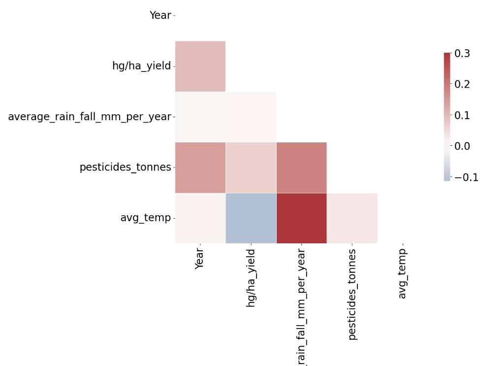
- Feature correlation analysis
import sklearn
import seaborn as sns
import matplotlib.pyplot as plt
correlation_data=yield_df.select_dtypes(include=[np.number]).corr()

mask = np.zeros_like(correlation_data, dtype=np.bool)
mask[np.triu_indices_from(mask)] = True

f, ax = plt.subplots(figsize=(11, 9))

# Generate a custom diverging colormap
cmap = sns.palette="vlag"

# Draw the heatmap with the mask and correct aspect ratio
sns.heatmap(correlation_data, mask=mask, cmap=cmap, vmax=.3, center=0,annot=True,
            square=True, linewidths=.5, cbar_kws={"shrink": .5});
- Data preparation for ML – One Hot Encoder, Min/Max Scaling, and Train/Test Split
from sklearn.preprocessing import OneHotEncoder
yield_df_onehot = pd.get_dummies(yield_df, columns=['Area',"Item"], prefix = ['Country',"Item"])
features=yield_df_onehot.loc[:, yield_df_onehot.columns != 'hg/ha_yield']
label=yield_df['hg/ha_yield']
features = features.drop(['Year'], axis=1)
from sklearn.preprocessing import MinMaxScaler
scaler=MinMaxScaler()
features=scaler.fit_transform(features)
from sklearn.model_selection import train_test_split
train_data, test_data, train_labels, test_labels = train_test_split(features, label, test_size=0.2, random_state=42)
- ML model training and testing
from sklearn.metrics import r2_score
def compare_models(model):
     model_name = model.__class__.__name__
     fit=model.fit(train_data,train_labels)
     y_pred=fit.predict(test_data)
     r2=r2_score(test_labels,y_pred)
     return([model_name,r2])
from sklearn.ensemble import RandomForestRegressor
from sklearn.ensemble import GradientBoostingRegressor
from sklearn import svm
from sklearn.tree import DecisionTreeRegressor

models = [
     GradientBoostingRegressor(n_estimators=200, max_depth=3, random_state=0),
      RandomForestRegressor(n_estimators=200, max_depth=3, random_state=0),
     svm.SVR(),
    DecisionTreeRegressor()
 ]
model_train=list(map(compare_models,models))
print(*model_train, sep = "\n")
['GradientBoostingRegressor', 0.8959545600619471]
['RandomForestRegressor', 0.6807690552605921]
['SVR', -0.19466686625412555]
['DecisionTreeRegressor', 0.959733560005363]
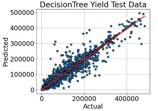
We select Decision Tree Regressor for ML training and testing.
yield_df_onehot = yield_df_onehot.drop(['Year'], axis=1)
#setting test data to columns from dataframe and excluding 'hg/ha_yield' values where ML model should be predicting

test_df=pd.DataFrame(test_data,columns=yield_df_onehot.loc[:, yield_df_onehot.columns != 'hg/ha_yield'].columns)

# using stack function to return a reshaped DataFrame by pivoting the columns of the current dataframe

cntry=test_df[[col for col in test_df.columns if 'Country' in col]].stack()[test_df[[col for col in test_df.columns if 'Country' in col]].stack()>0]
cntrylist=list(pd.DataFrame(cntry).index.get_level_values(1))
countries=[i.split("_")[1] for i in cntrylist]
itm=test_df[[col for col in test_df.columns if 'Item' in col]].stack()[test_df[[col for col in test_df.columns if 'Item' in col]].stack()>0]
itmlist=list(pd.DataFrame(itm).index.get_level_values(1))
items=[i.split("_")[1] for i in itmlist]
test_df.drop([col for col in test_df.columns if 'Item' in col],axis=1,inplace=True)
test_df.drop([col for col in test_df.columns if 'Country' in col],axis=1,inplace=True)

test_df['Country']=countries
test_df['Item']=items
from sklearn.tree import DecisionTreeRegressor
clf=DecisionTreeRegressor()
model=clf.fit(train_data,train_labels)

test_df["yield_predicted"]= model.predict(test_data)
test_df["yield_actual"]=pd.DataFrame(test_labels)["hg/ha_yield"].tolist()
test_group=test_df.groupby("Item")
# So let's run the model actual values against the predicted ones

fig, ax = plt.subplots()

ax.scatter(test_df["yield_actual"], test_df["yield_predicted"],edgecolors=(0, 0, 0))

ax.set_xlabel('Actual')
ax.set_ylabel('Predicted')
ax.set_title("DecisionTree Yield Test Data")

x=test_df["yield_actual"]
y=test_df["yield_predicted"]

m, b = np.polyfit(x, y, 1)

#add linear regression line to scatterplot
plt.plot(x, m*x+b,'r',lw=2)

plt.grid()
plt.show()
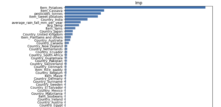
- Feature Importance Factor
varimp= {'imp':model.feature_importances_,'names':yield_df_onehot.columns[yield_df_onehot.columns!="hg/ha_yield"]}
a4_dims = (8.27,19)
plt.rcParams.update({'font.size': 10})
fig, ax = plt.subplots(figsize=a4_dims)
df=pd.DataFrame.from_dict(varimp)
df.sort_values(ascending=False,by=["imp"],inplace=True)
plt.title('Imp')
df=df.dropna()
sns.barplot(x="imp",y="names",palette="vlag",data=df,orient="h",ax=ax);
0.00 0.35
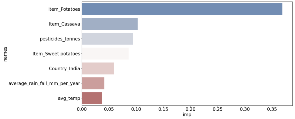
#7 most important factors that affect crops
a4_dims = (16.7, 8.27)
plt.rcParams.update({'font.size': 20})
fig, ax = plt.subplots(figsize=a4_dims)
df=pd.DataFrame.from_dict(varimp)
df.sort_values(ascending=False,by=["imp"],inplace=True)
df=df.dropna()
df=df.nlargest(7, 'imp')
sns.barplot(x="imp",y="names",palette="vlag",data=df,orient="h",ax=ax);
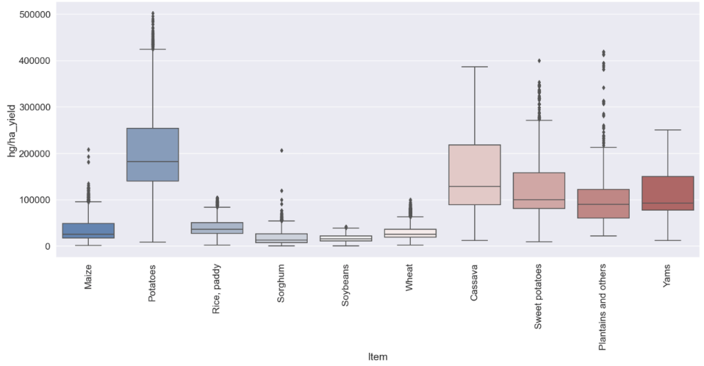
- Global Yield Prediction
#Boxplot that shows yield for each item
a4_dims = (20, 8)

fig, ax = plt.subplots(figsize=a4_dims)
sns.boxplot(x="Item",y="hg/ha_yield",palette="vlag",data=yield_df,ax=ax);
plt.xticks(rotation=90)
plt.savefig('yield_boxplot.png')
Crop Recommendation
- Here, we will implement the multi-label crop classification algorithm using the crop recommendation dataset DAT3. This is an important decision support tool for crop yield prediction, including supporting decisions on what crops to grow and what to do during the growing season of the crops.
- Key imports and input data loading
import pandas as pd # data analysis
import numpy as np # linear algebra

#import libraries for data visualization
import matplotlib.pyplot as plt
%matplotlib inline
import seaborn as sns
import plotly.graph_objects as go
import plotly.express as px
from plotly.subplots import make_subplots


from sklearn.metrics import classification_report
from sklearn import metrics
from sklearn import tree
from sklearn.model_selection import cross_val_score
import warnings
warnings.filterwarnings('ignore')
crop = pd.read_csv('Crop_recommendation.csv')
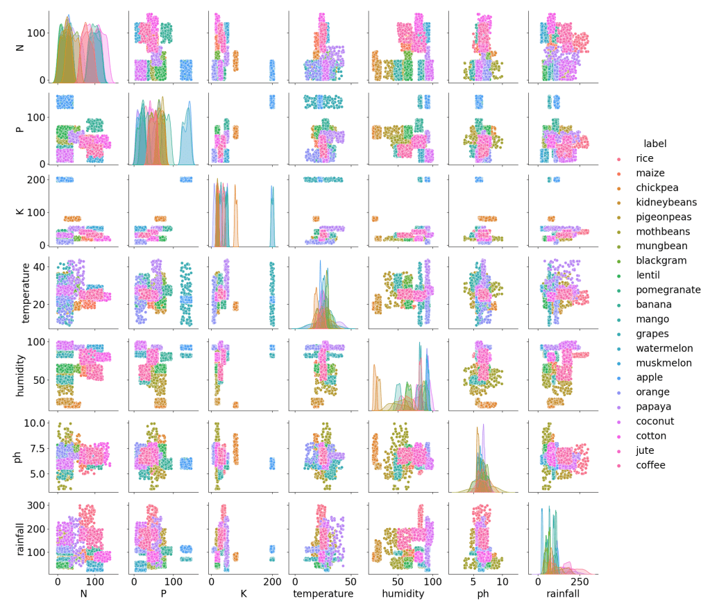
- Exploratory Data Analysis (EDA)
Pair plot of available features (K,P,N, temperature, humidity, pH, and rainfall) for different crop labels:
sns.pairplot(crop,hue = 'label')
plt.savefig('crop_pairplot.png')
Joint plot humidity vs rainfall for different crop labels:
plt.figure(figsize=(10,10))
sns.jointplot(x="rainfall",y="humidity",data=crop[(crop['temperature']<40) &
                                                  (crop['rainfall']>40)],height=10,hue="label")
plt.rcParams.update({'font.size': 12})
plt.savefig('crop_jointplot.png')

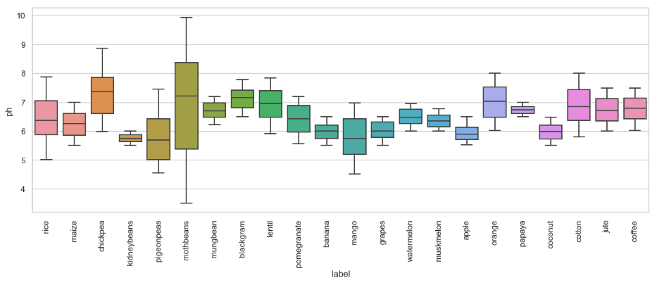
Box plots pH level vs crop labels:
sns.set_theme(style="whitegrid")
fig, ax = plt.subplots(figsize=(15,5))
sns.set(font_scale=1.5)
sns.boxplot(x='label',y='ph',data=crop)
plt.rcParams.update({'font.size': 22})
plt.xticks(rotation=90)
(array([ 0,  1,  2,  3,  4,  5,  6,  7,  8,  9, 10, 11, 12, 13, 14, 15, 16,
        17, 18, 19, 20, 21]),
 [Text(0, 0, 'rice'),
  Text(1, 0, 'maize'),
  Text(2, 0, 'chickpea'),
  Text(3, 0, 'kidneybeans'),
  Text(4, 0, 'pigeonpeas'),
  Text(5, 0, 'mothbeans'),
  Text(6, 0, 'mungbean'),
  Text(7, 0, 'blackgram'),
  Text(8, 0, 'lentil'),
  Text(9, 0, 'pomegranate'),
  Text(10, 0, 'banana'),
  Text(11, 0, 'mango'),
  Text(12, 0, 'grapes'),
  Text(13, 0, 'watermelon'),
  Text(14, 0, 'muskmelon'),
  Text(15, 0, 'apple'),
  Text(16, 0, 'orange'),
  Text(17, 0, 'papaya'),
  Text(18, 0, 'coconut'),
  Text(19, 0, 'cotton'),
  Text(20, 0, 'jute'),
  Text(21, 0, 'coffee')])
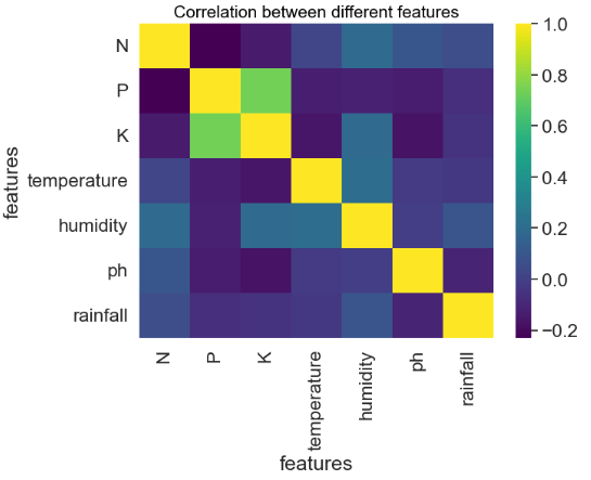
- Feature Correlation Matrix
Correlation between different features:
fig, ax = plt.subplots(1, 1, figsize=(7, 5))
plt.rcParams.update({'font.size': 20})
sns.set(font_scale=1.5)
sns.heatmap(crop.corr(), annot=False,cmap='viridis')
ax.set(xlabel='features')
ax.set(ylabel='features')

plt.title('Correlation between different features', fontsize = 15, c='black')
plt.savefig('corrmatrix0.png')
- Crop Summary Bar Plot
N-P-K values comparison between crops:
crop_summary = pd.pivot_table(crop,index=['label'],aggfunc='mean')
fig = go.Figure()
fig.add_trace(go.Bar(
    x=crop_summary.index,
    y=crop_summary['N'],
    name='Nitrogen',
    marker_color='mediumvioletred'
))
fig.add_trace(go.Bar(
    x=crop_summary.index,
    y=crop_summary['P'],
    name='Phosphorous',
    marker_color='springgreen'
))
fig.add_trace(go.Bar(
    x=crop_summary.index,
    y=crop_summary['K'],
    name='Potash',
    marker_color='dodgerblue'
))

fig.update_layout(title="N-P-K values comparison between crops",
                  plot_bgcolor='white',
                  barmode='group',
                  xaxis_tickangle=-45)

fig.show()

- ML Data Preparation
features = crop[['N', 'P','K','temperature', 'humidity', 'ph', 'rainfall']]
target = crop['label']
acc = []
model = []
from sklearn.model_selection import train_test_split
x_train, x_test, y_train, y_test = train_test_split(features,target,test_size = 0.3,random_state =2)
- K-Neighbors (KNN) Classifier
from sklearn.neighbors import KNeighborsClassifier
knn = KNeighborsClassifier()

knn.fit(x_train,y_train)

predicted_values = knn.predict(x_test)

x = metrics.accuracy_score(y_test, predicted_values)
acc.append(x)
model.append('K Nearest Neighbours')
print("KNN Accuracy is: ", x)

print(classification_report(y_test,predicted_values))
KNN Accuracy is:  0.9848484848484849
              precision    recall  f1-score   support

       apple       1.00      1.00      1.00        28
      banana       1.00      1.00      1.00        26
   blackgram       1.00      1.00      1.00        28
    chickpea       1.00      1.00      1.00        29
     coconut       1.00      1.00      1.00        31
      coffee       1.00      1.00      1.00        33
      cotton       0.97      1.00      0.98        31
      grapes       1.00      1.00      1.00        29
        jute       0.91      0.88      0.89        33
 kidneybeans       0.97      1.00      0.98        30
      lentil       0.97      1.00      0.98        32
       maize       1.00      0.97      0.98        32
       mango       1.00      1.00      1.00        33
   mothbeans       1.00      0.97      0.98        29
    mungbean       1.00      1.00      1.00        32
   muskmelon       1.00      1.00      1.00        30
      orange       1.00      1.00      1.00        42
      papaya       1.00      1.00      1.00        30
  pigeonpeas       1.00      0.97      0.98        31
 pomegranate       1.00      1.00      1.00        19
        rice       0.87      0.90      0.89        30
  watermelon       1.00      1.00      1.00        22

    accuracy                           0.98       660
   macro avg       0.99      0.99      0.99       660
weighted avg       0.99      0.98      0.98       660
score = cross_val_score(knn,features,target,cv=5)
print('Cross validation score: ',score)
Cross validation score: [0.97727273 0.98181818 0.97954545 0.97954545 0.97954545]
#Print Train Accuracy
knn_train_accuracy = knn.score(x_train,y_train)
print("knn_train_accuracy = ",knn.score(x_train,y_train))
#Print Test Accuracy
knn_test_accuracy = knn.score(x_test,y_test)
print("knn_test_accuracy = ",knn.score(x_test,y_test))
knn_train_accuracy =  0.9876623376623377
knn_test_accuracy =  0.9848484848484849
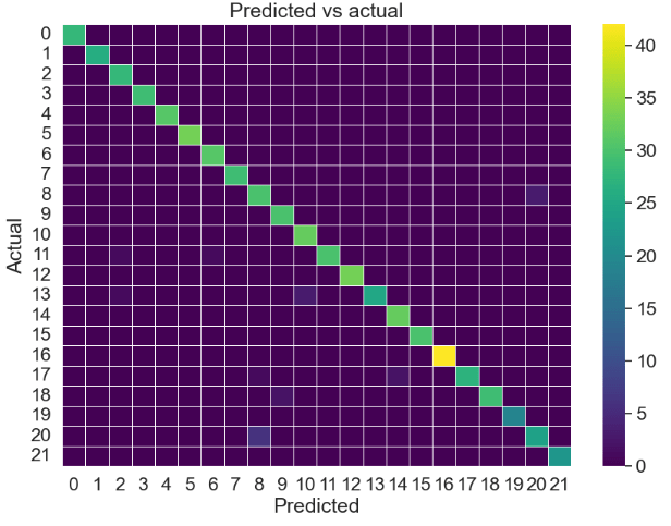
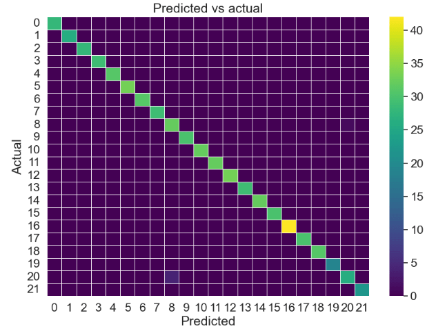
KNN confusion matrix:
y_pred = knn.predict(x_test)
y_true = y_test

from sklearn.metrics import confusion_matrix

cm_knn = confusion_matrix(y_true,y_pred)

f, ax = plt.subplots(figsize=(10,7))
sns.set(font_scale=1.5)
sns.heatmap(cm_knn, annot=False, linewidth=0.5, fmt=".0f",cmap='viridis', ax = ax)
plt.xlabel('Predicted')
plt.ylabel('Actual')
plt.title('Predicted vs actual')
plt.show()
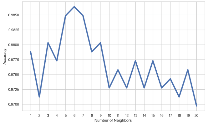
KNN Accuracy vs Number of Neighbors:
mean_acc = np.zeros(20)
for i in range(1,21):
    #Train Model and Predict
    knn = KNeighborsClassifier(n_neighbors = i).fit(x_train,y_train)
    yhat= knn.predict(x_test)
    mean_acc[i-1] = metrics.accuracy_score(y_test, yhat)
loc = np.arange(1,21,step=1.0)
plt.figure(figsize = (10, 6))
plt.plot(range(1,21), mean_acc,lw=4)
plt.xticks(loc)
plt.xlabel('Number of Neighbors ')
plt.ylabel('Accuracy')
plt.show()
- KNN HPO via Grid Search CV
from sklearn.model_selection import GridSearchCV
grid_params = { 'n_neighbors' : [6,9,11,13,15,17,19],
               'weights' : ['uniform','distance'],
               'metric' : ['minkowski','euclidean','manhattan']}
gs = GridSearchCV(KNeighborsClassifier(), grid_params, verbose = 1, cv=3, n_jobs = -1)
g_res = gs.fit(x_train, y_train)
Fitting 3 folds for each of 42 candidates, totalling 126 fits
g_res.best_score_
0.9844143071325814
g_res.best_params_
{'metric': 'manhattan', 'n_neighbors': 6, 'weights': 'distance'}
# Using the best hyperparameters
knn_1 = KNeighborsClassifier(n_neighbors = 6, weights = 'distance',algorithm = 'brute',metric = 'manhattan')
knn_1.fit(x_train, y_train)
                            KNeighborsClassifier
KNeighborsClassifier(algorithm='brute', metric='manhattan', n_neighbors=6,
                     weights='distance')
# Training & Testing accuracy after applying hyper parameter
knn_train_accuracy = knn_1.score(x_train,y_train)
print("knn_train_accuracy = ",knn_1.score(x_train,y_train))
#Print Test Accuracy
knn_test_accuracy = knn_1.score(x_test,y_test)
print("knn_test_accuracy = ",knn_1.score(x_test,y_test))
knn_train_accuracy =  1.0
knn_test_accuracy =  0.9818181818181818
- Decision Tree (DT) Classifier
from sklearn.tree import DecisionTreeClassifier
DT = DecisionTreeClassifier(criterion="entropy",random_state=2,max_depth=5)

DT.fit(x_train,y_train)

predicted_values = DT.predict(x_test)
x = metrics.accuracy_score(y_test, predicted_values)
acc.append(x)
model.append('Decision Tree')
print("Decision Tree's Accuracy is: ", x*100)

print(classification_report(y_test,predicted_values))
Decision Tree's Accuracy is:  85.9090909090909
              precision    recall  f1-score   support

       apple       1.00      1.00      1.00        28
      banana       1.00      1.00      1.00        26
   blackgram       0.65      1.00      0.79        28
    chickpea       1.00      1.00      1.00        29
     coconut       0.94      1.00      0.97        31
      coffee       1.00      1.00      1.00        33
      cotton       1.00      0.97      0.98        31
      grapes       1.00      1.00      1.00        29
        jute       0.50      0.03      0.06        33
 kidneybeans       0.00      0.00      0.00        30
      lentil       0.63      1.00      0.77        32
       maize       0.97      1.00      0.98        32
       mango       1.00      1.00      1.00        33
   mothbeans       0.00      0.00      0.00        29
    mungbean       1.00      1.00      1.00        32
   muskmelon       1.00      1.00      1.00        30
      orange       1.00      1.00      1.00        42
      papaya       1.00      1.00      1.00        30
  pigeonpeas       0.55      1.00      0.71        31
 pomegranate       1.00      1.00      1.00        19
        rice       0.49      0.97      0.65        30
  watermelon       1.00      1.00      1.00        22

    accuracy                           0.86       660
   macro avg       0.81      0.86      0.81       660
weighted avg       0.80      0.86      0.81       660
score = cross_val_score(DT, features, target,cv=5)
print('Cross validation score: ',score)
Cross validation score: [0.93636364 0.90909091 0.91818182 0.87045455 0.93636364]
#Print Train Accuracy
dt_train_accuracy = DT.score(x_train,y_train)
print("Training accuracy = ",DT.score(x_train,y_train))
#Print Test Accuracy
dt_test_accuracy = DT.score(x_test,y_test)
print("Testing accuracy = ",DT.score(x_test,y_test))
Training accuracy =  0.8675324675324675
Testing accuracy =  0.8590909090909091
Decision Tree confusion matrix:
y_pred = DT.predict(x_test)
y_true = y_test

from sklearn.metrics import confusion_matrix

cm_dt = confusion_matrix(y_true,y_pred)

f, ax = plt.subplots(figsize=(10,7))
sns.set(font_scale=1.5)
sns.heatmap(cm_dt, annot=False, linewidth=0.5, fmt=".0f",  cmap='viridis', ax = ax)
plt.xlabel("Predicted")
plt.ylabel("Actual")
plt.title('Predicted vs actual')
plt.show()

- Random Forest (RF) Classifier
from sklearn.ensemble import RandomForestClassifier

RF = RandomForestClassifier(n_estimators=20, random_state=0)
RF.fit(x_train,y_train)

predicted_values = RF.predict(x_test)

x = metrics.accuracy_score(y_test, predicted_values)
acc.append(x)
model.append('RF')
print("Random Forest Accuracy is: ", x)

print(classification_report(y_test,predicted_values))
Random Forest Accuracy is:  0.9893939393939394
              precision    recall  f1-score   support

       apple       1.00      1.00      1.00        28
      banana       1.00      1.00      1.00        26
   blackgram       0.97      1.00      0.98        28
    chickpea       1.00      1.00      1.00        29
     coconut       1.00      1.00      1.00        31
      coffee       1.00      1.00      1.00        33
      cotton       1.00      1.00      1.00        31
      grapes       1.00      1.00      1.00        29
        jute       0.89      0.94      0.91        33
 kidneybeans       1.00      1.00      1.00        30
      lentil       1.00      1.00      1.00        32
       maize       1.00      1.00      1.00        32
       mango       1.00      1.00      1.00        33
   mothbeans       1.00      0.97      0.98        29
    mungbean       1.00      1.00      1.00        32
   muskmelon       1.00      1.00      1.00        30
      orange       1.00      1.00      1.00        42
      papaya       1.00      1.00      1.00        30
  pigeonpeas       1.00      1.00      1.00        31
 pomegranate       1.00      1.00      1.00        19
        rice       0.93      0.87      0.90        30
  watermelon       1.00      1.00      1.00        22

    accuracy                           0.99       660
   macro avg       0.99      0.99      0.99       660
weighted avg       0.99      0.99      0.99       660
score = cross_val_score(RF,features,target,cv=5)
print('Cross validation score: ',score)
Cross validation score: [0.99772727 0.99545455 0.99772727 0.99318182 0.98863636]
#Print Train Accuracy
rf_train_accuracy = RF.score(x_train,y_train)
print("Training accuracy = ",RF.score(x_train,y_train))
#Print Test Accuracy
rf_test_accuracy = RF.score(x_test,y_test)
print("Testing accuracy = ",RF.score(x_test,y_test))
Training accuracy =  1.0
Testing accuracy =  0.9893939393939394
Random Forest confusion matrix:
y_pred = RF.predict(x_test)
y_true = y_test

from sklearn.metrics import confusion_matrix

cm_rf = confusion_matrix(y_true,y_pred)

f, ax = plt.subplots(figsize=(10,7))
sns.set(font_scale=1.5)
sns.heatmap(cm_rf, annot=False, linewidth=0.5, fmt=".0f",  cmap='viridis', ax = ax)
plt.xlabel("Predicted")
plt.ylabel("Actual")
plt.title('Predicted vs actual')
plt.show()

- Gaussian NB Classifier
from sklearn.naive_bayes import GaussianNB
NaiveBayes = GaussianNB()

NaiveBayes.fit(x_train,y_train)

predicted_values = NaiveBayes.predict(x_test)
x = metrics.accuracy_score(y_test, predicted_values)
acc.append(x)
model.append('Naive Bayes')
print("Naive Bayes Accuracy is: ", x)

print(classification_report(y_test,predicted_values))
Naive Bayes Accuracy is:  0.9924242424242424
              precision    recall  f1-score   support

       apple       1.00      1.00      1.00        28
      banana       1.00      1.00      1.00        26
   blackgram       1.00      1.00      1.00        28
    chickpea       1.00      1.00      1.00        29
     coconut       1.00      1.00      1.00        31
      coffee       1.00      1.00      1.00        33
      cotton       1.00      1.00      1.00        31
      grapes       1.00      1.00      1.00        29
        jute       0.89      0.97      0.93        33
 kidneybeans       1.00      1.00      1.00        30
      lentil       1.00      1.00      1.00        32
       maize       1.00      1.00      1.00        32
       mango       1.00      1.00      1.00        33
   mothbeans       1.00      1.00      1.00        29
    mungbean       1.00      1.00      1.00        32
   muskmelon       1.00      1.00      1.00        30
      orange       1.00      1.00      1.00        42
      papaya       1.00      1.00      1.00        30
  pigeonpeas       1.00      1.00      1.00        31
 pomegranate       1.00      1.00      1.00        19
        rice       0.96      0.87      0.91        30
  watermelon       1.00      1.00      1.00        22

    accuracy                           0.99       660
   macro avg       0.99      0.99      0.99       660
weighted avg       0.99      0.99      0.99       660
score = cross_val_score(NaiveBayes,features,target,cv=5)
print('Cross validation score: ',score)
Cross validation score: [0.99772727 0.99545455 0.99545455 0.99545455 0.99090909]
#Print Train Accuracy
nb_train_accuracy = NaiveBayes.score(x_train,y_train)
print("Training accuracy = ",NaiveBayes.score(x_train,y_train))
#Print Test Accuracy
nb_test_accuracy = NaiveBayes.score(x_test,y_test)
print("Testing accuracy = ",NaiveBayes.score(x_test,y_test))
Training accuracy =  0.9961038961038962
Testing accuracy =  0.9924242424242424
Naïve Bayes confusion matrix:
y_pred = NaiveBayes.predict(x_test)
y_true = y_test
sns.set(font_scale=1.5)

from sklearn.metrics import confusion_matrix

cm_nb = confusion_matrix(y_true,y_pred)

f, ax = plt.subplots(figsize=(10,7))
sns.heatmap(cm_nb, annot=False, linewidth=0.5, fmt=".0f",  cmap='viridis', ax = ax)
plt.xlabel("Predicted")
plt.ylabel("Actual")
plt.title('Predicted vs actual')
plt.show()
- Test ML Accuracy Score Bar Plot
plt.figure(figsize=[14,7],dpi = 100, facecolor='white')
sns.set(font_scale=2)
plt.title('Accuracy Comparison')
plt.xlabel('Accuracy')
plt.ylabel('ML Algorithms')
sns.barplot(x = acc,y = model,palette='viridis')
plt.savefig('plot.png', dpi=300, bbox_inches='tight')

- Testing vs Training ML Accuracy Comparison Bar Plot
label = ['KNN', 'Decision Tree','Random Forest','Naive Bayes']
Test = [knn_test_accuracy, dt_test_accuracy,rf_test_accuracy,
        nb_test_accuracy]
Train = [knn_train_accuracy,  dt_train_accuracy, rf_train_accuracy,
         nb_train_accuracy]

f, ax = plt.subplots(figsize=(20,7)) # set the size that you'd like (width, height)
X_axis = np.arange(len(label))
plt.bar(X_axis - 0.2,Test, 0.4, label = 'Test', color=('midnightblue'))
plt.bar(X_axis + 0.2,Train, 0.4, label = 'Train', color=('mediumaquamarine'))
plt.rcParams.update({'font.size': 20})
plt.xticks(X_axis, label)
plt.xlabel("ML algorithms")
plt.ylabel("Accuracy")
plt.title("Testing vs Training Accuracy")
plt.legend()
#plt.savefig('train vs test.png')
plt.show()

Effects of Climate Changes
- Finally, we will examine the effect of climate changes on crop yields worldwide.
- The input dataset DAT4 describes Effects of Climate Changes on Crop Yields worldwide.
- This dataset has 7 columns and 28242 rows.
Area
Item
Year
average_rain_fall_mm_per_year
pesticides_tonnes
avg_temp
hg/ha_yield
- Basic imports and load the input dataset
import pandas as pd
import numpy as np
import matplotlib.pyplot as plt
import matplotlib.colors as mcolors
import seaborn as sns
%matplotlib inline
df=pd.read_csv('climate-ds.csv',index_col=0)
- Evaluation functions for regression models
from sklearn.metrics import mean_absolute_error, mean_squared_error, max_error, median_absolute_error, r2_score, explained_variance_score, mean_absolute_percentage_error
import numpy as np
from sklearn.model_selection import GridSearchCV, RandomizedSearchCV
#Evaluation function for regression models
def regression_report(y_true, y_pred):

    error = y_true - y_pred

    #Evaluation matrics
    mae = mean_absolute_error(y_true, y_pred)
    medae = median_absolute_error(y_true, y_pred)
    mse = mean_squared_error(y_true, y_pred)
    rmse = np.sqrt(mean_squared_error(y_true, y_pred))
    maxerr = max_error(y_true, y_pred)
    r_squared = r2_score(y_true, y_pred)
    evs = explained_variance_score(y_true, y_pred)
    mape = mean_absolute_percentage_error(y_true, y_pred)
    metrics = [
        ('Mean Absolute Error', mae),
        ('Median Absolute Error', medae),
        ('Mean Squared Error', mse),
        ('Root Mean Squared Error', rmse),
        ('Max error', maxerr) ,
        ('R2 score', r_squared),
        ('Explained variance score', evs),
        ('Mean Absolute Percentage Error', mape)
    ]

    print('Regression Report:')
    for metric_name, metric_value in metrics:
        print(f'\t\t\t{metric_name:30s}: {metric_value: >20.3f}')

    return mae, medae, mse, rmse, maxerr, r_squared, evs, mape
- ML data preparation
#remove Duplicates
df.drop_duplicates(keep='first',inplace = True)
#one hot encoding for the categorical columns to can be trained in the model
df = pd.get_dummies(df,columns=['Area','Item'])
df.rename(columns={x:x[5:] for x in df.columns[6:]}, inplace = True)
#split the data into the target and labels
x = df.drop(labels=['hg/ha_yield'], axis=1)
y = df['hg/ha_yield']
#Scaling
from sklearn.preprocessing import StandardScaler
scaler = StandardScaler()

x = scaler.fit_transform(x)
#Split the data into the train and test datasets as 80:20 %
#split data to x_train, x_test, y_train, y_test
from sklearn.model_selection import train_test_split
x_train, x_test, y_train, y_test = train_test_split(x, y, test_size=0.20, random_state=40,shuffle=True)
#Make DataFrame for track model accuracy
df_models = pd.DataFrame(columns=["Model", "MAE","MEDAE","MSE","RMSE", "Max Error","R2 Score","EVS","MAPE"])
- LGBM Regressor + Randomized Search CV
import lightgbm as lgb
import scipy as sp
lgbm = lgb.LGBMRegressor(
                             objective='regression',
                             n_jobs=1,
                            )
#dictionary for hyper parameters
param_dist = {'boosting_type': ['gbdt', 'dart', 'rf'],
                    'num_leaves': sp.stats.randint(2, 1001),
                    'subsample_for_bin': sp.stats.randint(10, 1001),
                    'min_split_gain': sp.stats.uniform(0, 5.0),
                    'min_child_weight': sp.stats.uniform(1e-6, 1e-2),
                    'reg_alpha': sp.stats.uniform(0, 1e-2),
                    'reg_lambda': sp.stats.uniform(0, 1e-2),
                    'tree_learner': ['data', 'feature', 'serial', 'voting' ],
                    'application': ['regression_l1', 'regression_l2', 'regression'],
                    'bagging_freq': sp.stats.randint(1, 11),
                    'bagging_fraction': sp.stats.uniform(1e-3, 0.99),
                    'feature_fraction': sp.stats.uniform(1e-3, 0.99),
                    'learning_rate': sp.stats.uniform(1e-6, 0.99),
                    'max_depth': sp.stats.randint(1, 501),
                    'n_estimators': sp.stats.randint(100, 20001),
                 }
rscv = RandomizedSearchCV(
                              estimator=lgbm,
                              param_distributions=param_dist,
                              cv=3,
                              verbose=0
                            )
rscv.fit(x_train, y_train)
print("The best parameters are %s with a score of %0.2f"
      % (rscv.best_params_, rscv.best_score_))
gbr_pred = rscv.predict(x_test)
mae, medae, mse, rmse, maxerr, r_squared, evs, mape = regression_report(y_test, gbr_pred)
row = {"Model": "GBRegressor", "MAE": mae,"MEDAE": medae, "MSE": mse, "RMSE": rmse,
           "Max Error": maxerr, "R2 Score": r_squared, "EVS": evs, "MAPE": mape}
df_models = df_models.append(row, ignore_index=True)
The best parameters are {'application': 'regression_l2', 'bagging_fraction': 0.32615789951845936, 'bagging_freq': 5, 'boosting_type': 'gbdt', 'feature_fraction': 0.6168548991646009, 'learning_rate': 0.10299929691491512, 'max_depth': 442, 'min_child_weight': 0.007374638179549023, 'min_split_gain': 1.8189493243011623, 'n_estimators': 10896, 'num_leaves': 128, 'reg_alpha': 0.007666291745158882, 'reg_lambda': 0.0004935270085926446, 'subsample_for_bin': 63, 'tree_learner': 'voting'} with a score of 0.97
Regression Report:
			Mean Absolute Error           :             5611.731
			Median Absolute Error         :             2451.671
			Mean Squared Error            :        119179650.226
			Root Mean Squared Error       :            10916.943
			Max error                     :           140538.210
			R2 score                      :                0.984
			Explained variance score      :                0.984
			Mean Absolute Percentage Error:                0.166
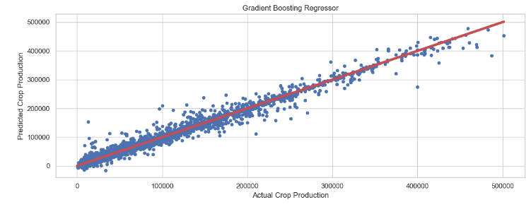
Gradient Boosting Regressor: Actual Crop Production vs Predicted Crop Production
plt.figure(figsize=(12,5))
plt.rcParams.update({'font.size': 22})
plt.scatter(y_test, gbr_pred, s=20)
plt.title('Gradient Boosting Regressor')
plt.xlabel('Actual Crop Production')
plt.ylabel('Predicted Crop Production')

plt.plot([min(y_test), max(y_test)], [min(y_test), max(y_test)], color='r', linewidth = 4)
plt.tight_layout()
- SGD Regressor + Grid Search CV
from sklearn.linear_model import SGDRegressor
param_grid = {
    'learning_rate': ['constant', "optimal", "invscaling", "adaptive" ]
}
sgd = SGDRegressor()
model = GridSearchCV(estimator=sgd, param_grid=param_grid, cv=5,verbose=0)
model.fit(x_train, y_train)
sgd_pred = model.predict(x_test)
mae, medae, mse, rmse, maxerr, r_squared, evs, mape = regression_report(y_test, sgd_pred)
row = {"Model": "SGDRegressor", "MAE": mae,"MEDAE": medae, "MSE": mse, "RMSE": rmse,
           "Max Error": maxerr, "R2 Score": r_squared, "EVS": evs, "MAPE": mape}
df_models = df_models.append(row, ignore_index=True)
Regression Report:
			Mean Absolute Error           :            30368.905
			Median Absolute Error         :            21651.677
			Mean Squared Error            :       1848725829.406
			Root Mean Squared Error       :            42996.812
			Max error                     :           293166.963
			R2 score                      :                0.744
			Explained variance score      :                0.744
			Mean Absolute Percentage Error:                0.961
SGD Regressor: Actual Crop Production vs Predicted Crop Production
plt.figure(figsize=(15,7))
plt.scatter(y_test, sgd_pred, s=20)
plt.title('SGD Regression',fontsize=20)
plt.xlabel('Actual Crop Production',fontsize=15)
plt.ylabel('Predicted Crop Production',fontsize=15)

plt.plot([min(y_test), max(y_test)], [min(y_test), max(y_test)], color='r', linewidth = 4)
plt.tight_layout()

- Ridge Regressor + Grid Search CV
from sklearn.linear_model import Ridge
param_grid = {
    'alpha': [0.001, 0.01, 0.1, 1, 2, 3, 4, 5]
}
rid = Ridge()
model = GridSearchCV(estimator=rid, param_grid=param_grid, cv=5, verbose=0)
model.fit(x_train, y_train)
GridSearchCV(cv=5, estimator=Ridge(),
             param_grid={'alpha': [0.001, 0.01, 0.1, 1, 2, 3, 4, 5]})
print("The best parameters are %s with a score of %0.2f"
      % (model.best_params_, model.best_score_))
rid_pred = model.predict(x_test)
mae, medae, mse, rmse, maxerr, r_squared, evs, mape = regression_report(y_test, rid_pred)
row = {"Model": "RidgeRegression", "MAE": mae,"MEDAE": medae, "MSE": mse, "RMSE": rmse,
           "Max Error": maxerr, "R2 Score": r_squared, "EVS": evs, "MAPE": mape}
df_models = df_models.append(row, ignore_index=True)
The best parameters are {'alpha': 5} with a score of 0.75
Regression Report:
			Mean Absolute Error           :            30366.278
			Median Absolute Error         :            21672.704
			Mean Squared Error            :       1848693387.670
			Root Mean Squared Error       :            42996.435
			Max error                     :           293175.625
			R2 score                      :                0.744
			Explained variance score      :                0.744
			Mean Absolute Percentage Error:                0.961
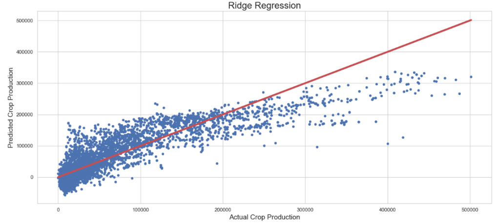
Ridge Regressor: Actual Crop Production vs Predicted Crop Production
plt.figure(figsize=(15,7))
plt.scatter(y_test, rid_pred, s=20)
plt.title('Ridge Regression',fontsize=20)
plt.xlabel('Actual Crop Production',fontsize=15)
plt.ylabel('Predicted Crop Production',fontsize=15)

plt.plot([min(y_test), max(y_test)], [min(y_test), max(y_test)], color='r', linewidth = 4)
plt.tight_layout()
- Lasso Regression
from sklearn.linear_model import Lasso
model = Lasso(alpha= 2, max_iter=10000, tol=0.001)
model.fit(x_train, y_train)
lass_pred = model.predict(x_test)
mae, medae, mse, rmse, maxerr, r_squared, evs, mape = regression_report(y_test, lass_pred)
row = {"Model": "LassoRegression", "MAE": mae,"MEDAE": medae, "MSE": mse, "RMSE": rmse,
           "Max Error": maxerr, "R2 Score": r_squared, "EVS": evs, "MAPE": mape}
df_models = df_models.append(row, ignore_index=True)
Regression Report:
			Mean Absolute Error           :            30365.686
			Median Absolute Error         :            21654.177
			Mean Squared Error            :       1848719390.779
			Root Mean Squared Error       :            42996.737
			Max error                     :           293146.259
			R2 score                      :                0.744
			Explained variance score      :                0.744
			Mean Absolute Percentage Error:                0.961
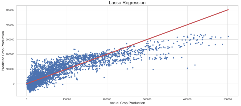
Lasso Regressor: Actual Crop Production vs Predicted Crop Production
plt.figure(figsize=(15,7))
plt.scatter(y_test, lass_pred, s=20)
plt.title('Lasso Regression',fontsize=20)
plt.xlabel('Actual Crop Production',fontsize=15)
plt.ylabel('Predicted Crop Production',fontsize=15)

plt.plot([min(y_test), max(y_test)], [min(y_test), max(y_test)], color='r', linewidth = 4)
plt.tight_layout()
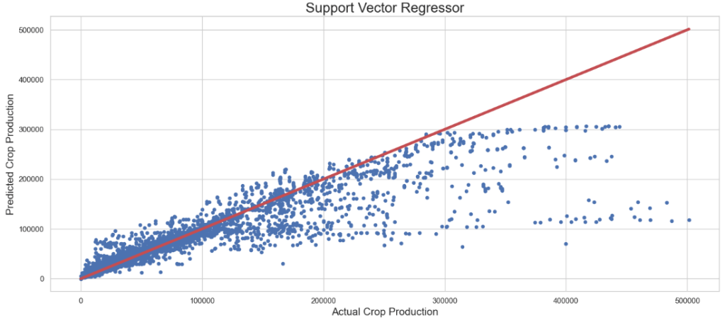
- SVR + Randomized Search CV
from sklearn.svm import SVR
param_dist = {
    'kernel' : ['rbf'],
    'C' : sp.stats.randint(1, 10001),
    "epsilon" : sp.stats.uniform(0.00001, 0.99),
    'gamma' : ['scale', 'auto']
}

svr = SVR()
svrcv = RandomizedSearchCV(
                              estimator=svr,
                              param_distributions=param_dist,
                              cv=3,
                              verbose=0
                            )
svrcv.fit(x_train, y_train)
print("The best parameters are %s with a score of %0.2f"
      % (svrcv.best_params_, svrcv.best_score_))
The best parameters are {'C': 9798, 'epsilon': 0.9537504981825164, 'gamma': 'auto', 'kernel': 'rbf'} with a score of 0.75
svrc_pred = svrcv.predict(x_test)
SVR + Randomized Search CV: Actual Crop Production vs Predicted Crop Production
plt.figure(figsize=(15,7))
plt.scatter(y_test, svrc_pred, s=20)
plt.title('Support Vector Regressor',fontsize=20)
plt.xlabel('Actual Crop Production',fontsize=15)
plt.ylabel('Predicted Crop Production',fontsize=15)

plt.plot([min(y_test), max(y_test)], [min(y_test), max(y_test)], color='r', linewidth = 4)
plt.tight_layout()
- Elastic Net Regression
from sklearn.linear_model import ElasticNet
model = ElasticNet()
model.fit(x_train, y_train)
en_pred = model.predict(x_test)
mae, medae, mse, rmse, maxerr, r_squared, evs, mape = regression_report(y_test, en_pred)
row = {"Model": "ElasticNet", "MAE": mae,"MEDAE": medae, "MSE": mse, "RMSE": rmse,
           "Max Error": maxerr, "R2 Score": r_squared, "EVS": evs, "MAPE": mape}
df_models = df_models.append(row, ignore_index=True)
Regression Report:
			Mean Absolute Error           :            31848.603
			Median Absolute Error         :            20473.156
			Mean Squared Error            :       2373038555.698
			Root Mean Squared Error       :            48713.844
			Max error                     :           314896.007
			R2 score                      :                0.672
			Explained variance score      :                0.672
			Mean Absolute Percentage Error:                1.082
Elastic Net Regression: Actual Crop Production vs Predicted Crop Production
plt.figure(figsize=(15,7))
plt.scatter(y_test, en_pred, s=20)
plt.title('Elastic Net',fontsize=20)
plt.xlabel('Actual Crop Production',fontsize=15)
plt.ylabel('Predicted Crop Production',fontsize=15)

plt.plot([min(y_test), max(y_test)], [min(y_test), max(y_test)], color='r', linewidth = 4)
plt.tight_layout()
- Random Forest Regressor + Randomized Search CV
from sklearn.ensemble import RandomForestRegressor
# Create the random grid
random_grid = {'n_estimators': [int(x) for x in np.linspace(start = 100, stop = 1200, num = 12)],
               'max_features': ['auto', 'sqrt'],
               'max_depth': [int(x) for x in np.linspace(5, 30, num = 6)],
               'min_samples_split': [2, 5, 10, 15, 100],
               'min_samples_leaf': [1, 2, 5, 10],
               'bootstrap' : [True, False]
              }
rfr = RandomForestRegressor()
rfrcv = RandomizedSearchCV(
                              estimator=rfr,
                              param_distributions=random_grid,
                              cv=3,
                              verbose=0
                            )
rfrcv.fit(x_train, y_train)
RandomizedSearchCV(cv=3, estimator=RandomForestRegressor(),
                   param_distributions={'bootstrap': [True, False],
                                        'max_depth': [5, 10, 15, 20, 25, 30],
                                        'max_features': ['auto', 'sqrt'],
                                        'min_samples_leaf': [1, 2, 5, 10],
                                        'min_samples_split': [2, 5, 10, 15,
                                                              100],
                                        'n_estimators': [100, 200, 300, 400,
                                                         500, 600, 700, 800,
                                                         900, 1000, 1100,
                                                         1200]})
print("The best parameters are %s with a score of %0.2f"
      % (rfrcv.best_params_, rfrcv.best_score_))
rfr_pred = rfrcv.predict(x_test)
mae, medae, mse, rmse, maxerr, r_squared, evs, mape = regression_report(y_test, rfr_pred)
row = {"Model": "RandomForestRegressor", "MAE": mae,"MEDAE": medae, "MSE": mse, "RMSE": rmse,
           "Max Error": maxerr, "R2 Score": r_squared, "EVS": evs, "MAPE": mape}
df_models = df_models.append(row, ignore_index=True)
The best parameters are {'n_estimators': 1000, 'min_samples_split': 100, 'min_samples_leaf': 1, 'max_features': 'sqrt', 'max_depth': 30, 'bootstrap': False} with a score of 0.92
Regression Report:
			Mean Absolute Error           :            12283.925
			Median Absolute Error         :             6875.181
			Mean Squared Error            :        427473740.868
			Root Mean Squared Error       :            20675.438
			Max error                     :           239840.455
			R2 score                      :                0.941
			Explained variance score      :                0.941
			Mean Absolute Percentage Error:                0.422
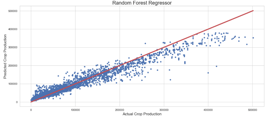
Random Forest Regressor + Randomized Search CV: Actual Crop Production vs Predicted Crop Production
plt.figure(figsize=(15,7))
plt.scatter(y_test, rfr_pred, s=20)
plt.title('Random Forest Regressor',fontsize=20)
plt.xlabel('Actual Crop Production',fontsize=15)
plt.ylabel('Predicted Crop Production',fontsize=15)

plt.plot([min(y_test), max(y_test)], [min(y_test), max(y_test)], color='r', linewidth = 4)
plt.tight_layout()
- XGB Regressor + HPO
from xgboost import XGBRegressor
from hyperopt import hp, fmin, tpe, STATUS_OK, Trials
space={'max_depth': hp.quniform("max_depth", 3, 18, 1),
        'learning_rate': hp.loguniform('learning_rate', np.log(0.001), np.log(0.5)),
        'gamma': hp.uniform ('gamma', 1,9),
        'reg_alpha' : hp.uniform('reg_alpha', 0.001, 1.0),
        'reg_lambda' : hp.uniform('reg_lambda', 0,1),
        'colsample_bytree' : hp.uniform('colsample_bytree', 0.5,1),
        'min_child_weight' : hp.quniform('min_child_weight', 0, 10, 1),
        'n_estimators': hp.uniform("n_estimators", 100, 20001)
    }
def objective(space):
    rego=XGBRegressor(
                    n_estimators =int(space['n_estimators']), max_depth = int(space['max_depth']),
                    learning_rate = space['learning_rate'], gamma = space['gamma'],
                    reg_alpha = space['reg_alpha'], min_child_weight=int(space['min_child_weight']),
                    reg_lambda = space['reg_lambda'],
                    colsample_bytree=int(space['colsample_bytree']), eval_metric="rmse",
                    early_stopping_rounds=10)

    evaluation = [( x_train, y_train), ( x_test, y_test)]

    rego.fit(x_train, y_train,
            eval_set=evaluation, verbose=0)


    y_pred = rego.predict(x_test)
    r_squared = r2_score(y_test, y_pred)
    return {'loss': -r_squared, 'status': STATUS_OK }
trials = Trials()

best_hyperparams = fmin(fn = objective,
                        space = space,
                        algo = tpe.suggest,
                        max_evals = 100,
                        trials = trials)
best_hyperparams['max_depth'],best_hyperparams['n_estimators'] = int(best_hyperparams['max_depth']),int(best_hyperparams['n_estimators'])
model = XGBRegressor(**best_hyperparams)
model.fit(x_train, y_train)
xgb_pred = model.predict(x_test)
mae, medae, mse, rmse, maxerr, r_squared, evs, mape = regression_report(y_test, xgb_pred)
row = {"Model": "XGBRegressor", "MAE": mae,"MEDAE": medae, "MSE": mse, "RMSE": rmse,
           "Max Error": maxerr, "R2 Score": r_squared, "EVS": evs, "MAPE": mape}
df_models = df_models.append(row, ignore_index=True)
Regression Report:
			Mean Absolute Error           :             7784.185
			Median Absolute Error         :             4403.359
			Mean Squared Error            :        177196950.303
			Root Mean Squared Error       :            13311.534
			Max error                     :           213066.703
			R2 score                      :                0.975
			Explained variance score      :                0.976
			Mean Absolute Percentage Error:                0.237
XGB Regressor + HPO: Actual Crop Production vs Predicted Crop Production
plt.figure(figsize=(15,7))
plt.scatter(y_test, xgb_pred, s=20)
plt.title('XGB Regressor',fontsize=20)
plt.xlabel('Actual Crop Production',fontsize=15)
plt.ylabel('Predicted Crop Production',fontsize=15)

plt.plot([min(y_test), max(y_test)], [min(y_test), max(y_test)], color='r', linewidth = 4)
plt.tight_layout()

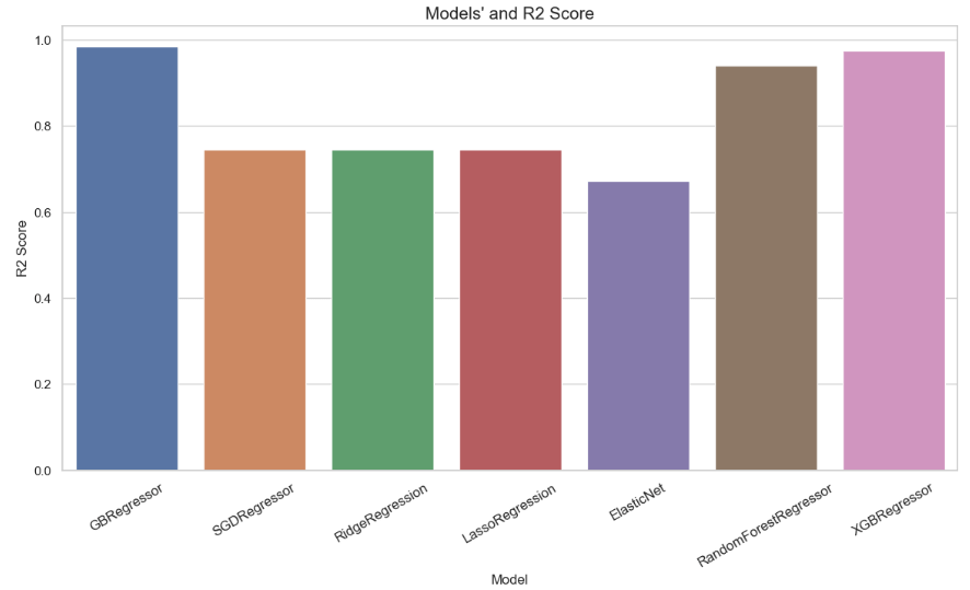
- QC Comparison of 7 Regression Models
df_models.sort_values(by="R2 Score")

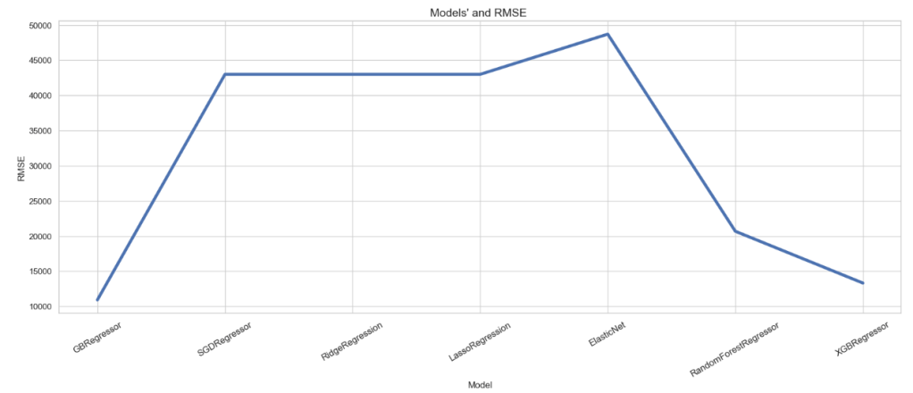
R2-Score of 7 Regression Models
RMSE of Regression Models
plt.figure(figsize=(20,7))
sns.lineplot(x=df_models.Model, y=df_models.RMSE,lw=4)
plt.title("Models' and RMSE ", size=15)
plt.xticks(rotation=30, size=12)
plt.show()
Summary
- We have addressed the ML-based crop yield prediction. This is an essential predictive analytics technique in the agriculture industry. It is an agricultural practice that can help farmers and farming businesses predict crop yield in a particular season when to plant a crop, and when to harvest for better crop yield.
- Several ML algorithms have been applied to support crop yield prediction studies. We have performed a systematic QC comparison of these algorithms using 4 public-domain datasets (courtesy of FAO and World Data Bank).
- CatBoost/SHAP Indian Crop Yield: top SHAP value for log10 yield is Coconut, CatBoost Regressor RMSE score for train is 0.152 dex and for test is 0.168 dex, top season is summer, and top state is Delphi.
- ML-Powered Indian Agriculture:
| Train/Test Data | Algorithm | R2-Score Train | R2-Score Test |
| After Transform + VIF | Random Forest Regressor | 0.99 | 0.95 |
- Global Crop Yield Prediction: the predicted-Actual Yield Test data X-plot is reasonable for the Decision tree algorithm; top yield predictions are potatoes, sweet potatoes, and cassava.
- Crop Recommendation: Multi-label classification of 21 crops leads to severe data overfitting ; Naïve Bayes and RF are the best performers in terms of Accuracy.
- Effects of Climate Changes: Best performers are XGB and GB regressors with HPO and R2-scores of 0.97 and 0.98, respectively.
- However, ML crop yield forecasting is still challenging due to the many factors involved, such as crop and variety, soil type, management practices, pests and diseases, and climate and weather patterns during the season.
- The Road Ahead: Crop Yield Prediction Using ML And Flask Deployment.
Explore More


Make a one-time donation
Make a monthly donation
Make a yearly donation
Choose an amount
Or enter a custom amount
Your contribution is appreciated.
Your contribution is appreciated.
Your contribution is appreciated.
DonateDonate monthlyDonate yearly
Leave a comment