
- In the green energy sector, being able to forecast the electricity usage is a core part of any electricity retailer’s business.
- The business problem is as follows: Given the historical power consumption, what is the expected power consumption for the next 365 days?
- In this study, we will address the problem by building a reliable Time Series Forecasting (TSF) model for hourly U.S.A. energy consumption.
- Our first objective (Part 1) is to compare several available TSF techniques such as TSF LSTM, supervised ML regressors (e.g. XGBoost), and FB Prophet.
- For a better interpretation of seasonal time series, multi-seasonal TSF methods have been developed such as the Unobserved Components Model (UCM). Therefore, our second objective (Part 2) is to focus on comprehensive testing and validation of UCM to gain additional insights into power demand dynamics and to forecast energy demand one year ahead using the available past values.
- Part 1 represents a showcase TSF using the PJM East Region dataset PJME_hourly.csv.
- To compare results of Deep Learning RNN and LSTM (Part 1), we consider the DOM_hourly.csv data.
- To demonstrate the power of UCM (Part 2), we select the American Electric Power (AEP) time series AEP_hourly.csv (from 10.01.2004 01:00:00 to 03.08.2018. 00:00:00).
Table of Contents
- PJME Data
- Data Preparation
- LSTM TSF
- XGBoost TSF
- FB Prophet TSF
- DOM Data
- RNN TSF
- LSTM TSF
- AEP Data
- Multi-Seasonal TSF
- UCM Approximations
- UCM Residual Diagnostics
- Summary
- Explore More
PJME Data
Let’s set the working directory YOURPATH
import os
os.chdir('YOURPATH')    # Set working directory
os. getcwd()
and import the following key libraries
import numpy as np # linear algebra
import pandas as pd # data processing, CSV file I/O (e.g. pd.read_csv)
import numpy as np
from numpy import concatenate
import urllib.request as urllib
from sklearn.preprocessing import StandardScaler, MinMaxScaler, LabelEncoder, OneHotEncoder
from sklearn.model_selection import train_test_split
from sklearn.metrics import mean_squared_error
from keras.models import Sequential
from keras.layers import Dense

import seaborn as sns
import matplotlib.pyplot as plt
from math import sqrt

from sklearn.metrics import mean_squared_error,mean_absolute_error
from keras.models import Sequential
from keras.layers import Dense,Dropout
from keras.layers import LSTM
Let’s read the input csv file in our working directory
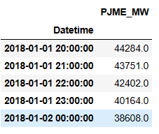
data = pd.read_csv('PJME_hourly.csv',index_col=[0], parse_dates=[0])
data.tail()
Let’s plot the time series
import seaborn as sns
sns.set(rc={'figure.figsize':(11, 5)})
data['PJME_MW'].plot(linewidth=0.5).set(title='PJME_MW')

Data Preparation
def create_features(df, label=None):
"""
Creates time series features from datetime index.
"""
df = df.copy()
df['date'] = df.index
df['hour'] = df['date'].dt.hour
df['dayofweek'] = df['date'].dt.dayofweek
df['quarter'] = df['date'].dt.quarter
df['month'] = df['date'].dt.month
df['year'] = df['date'].dt.year
df['dayofyear'] = df['date'].dt.dayofyear
df['dayofmonth'] = df['date'].dt.day
df['weekofyear'] = df['date'].dt.weekofyear
X = df[['hour','dayofweek','quarter','month','year',
'dayofyear','dayofmonth','weekofyear']]
if label:
y = df[label]
return X, y
return X
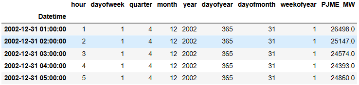
X, y = create_features(data, label='PJME_MW')
df = pd.concat([X, y], axis=1)
df.tail()

# convert series to supervised learning
def series_to_supervised(data, n_in=1, n_out=1, dropnan=True):
	n_vars = 1 if type(data) is list else data.shape[1]
	df = pd.DataFrame(data)
	cols, names = list(), list()
	# input sequence (t-n, ... t-1)
	for i in range(n_in, 0, -1):
		cols.append(df.shift(i))
		names += [('var%d(t-%d)' % (j+1, i)) for j in range(n_vars)]
	# forecast sequence (t, t+1, ... t+n)
	for i in range(0, n_out):
		cols.append(df.shift(-i))
		if i == 0:
			names += [('var%d(t)' % (j+1)) for j in range(n_vars)]
		else:
			names += [('var%d(t+%d)' % (j+1, i)) for j in range(n_vars)]
	# put it all together
	agg = pd.concat(cols, axis=1)
	agg.columns = names
	# drop rows with NaN values
	#if dropnan:
		#agg.dropna(inplace=True)
	return agg
# Preprocess data
labelEncoder = LabelEncoder()
oneHotEncoder = OneHotEncoder()
ss = StandardScaler()

values = df.values
# integer encode direction
#encoder = LabelEncoder()
#values[:,8] = encoder.fit_transform(values[:,8])
# ensure all data is float
values = values.astype('float32')
# normalize features
scaler = MinMaxScaler(feature_range=(0, 1))
scaled = scaler.fit_transform(values)

# frame as supervised learning
reframed = series_to_supervised(scaled, 1, 1)
# drop columns we don't want to predict
reframed.drop(reframed.columns[[9,10,11,12,13,14,15,16]], axis=1, inplace=True)
# split into train and test sets
reframed['date_time'] = df.index.values
split_date = '01-Jan-2015'

train = reframed.loc[reframed['date_time']<=split_date].drop(['date_time'],axis=1).dropna().values
test = reframed.loc[reframed['date_time']>split_date].drop(['date_time'],axis=1).dropna().values

# split into input and output
X_train, y_train = train[:, 0:-1], train[:, -1]
X_test, y_test = test[:, 0:-1], test[:, -1]
# reshape input to be 3D [samples, timesteps, features]
X_train = X_train.reshape((X_train.shape[0], 1, X_train.shape[1]))
X_test = X_test.reshape((X_test.shape[0], 1, X_test.shape[1]))
print(X_train.shape, y_train.shape, X_test.shape, y_test.shape)
Output: (113926, 1, 9) (113926,) (31439, 1, 9) (31439,)
LSTM TSF
# design network
model = Sequential()
model.add(LSTM(100, input_shape=(X_train.shape[1], X_train.shape[2])))
model.add(Dropout(0.2))
model.add(Dense(1))
model.compile(loss='mae', optimizer='adam')
# fit network
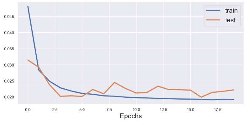
history = model.fit(X_train, y_train, epochs=20, batch_size=70, validation_data=(X_test, y_test), verbose=2, shuffle=False)
Let’s plot the LSTM train/test val_loss history
from matplotlib import pyplot as plt
import matplotlib
matplotlib.rcParams.update({'font.size': 20})
# plot history
plt.plot(history.history['loss'], label='train',lw=3)
plt.plot(history.history['val_loss'], label='test',lw=3)
plt.legend(fontsize=18)
plt.xlabel('Epochs',fontsize=18)
plt.show()
# make a prediction
yhat = model.predict(X_test)
X_test = X_test.reshape((X_test.shape[0], X_test.shape[2]))
# invert scaling for forecast
inv_yhat = concatenate((X_test[:,:-1],yhat), axis=1)
inv_yhat = scaler.inverse_transform(inv_yhat)
inv_yhat = inv_yhat[:,-1]
# invert scaling for actual
y_test = y_test.reshape((len(y_test), 1))
inv_y = concatenate((X_test[:,:-1],y_test), axis=1)
inv_y = scaler.inverse_transform(inv_y)
inv_y = inv_y[:,-1]
# calculate RMSE
MSE=mean_squared_error(inv_y,inv_yhat)
MAE=mean_absolute_error(inv_y,inv_yhat)
RMSE = sqrt(mean_squared_error(inv_y, inv_yhat))
print('MSE: %.3f' % MSE + '   MAE: %.3f' % MAE + '   RMSE: %.3f' % RMSE)
Output:
MSE: 1811223.125 MAE: 1053.133 RMSE: 1345.817
def mean_absolute_percentage_error(y_true, y_pred):
    """Calculates MAPE given y_true and y_pred"""
    y_true, y_pred = np.array(y_true), np.array(y_pred)
    return np.mean(np.abs((y_true - y_pred) / y_true)) * 100

print(mean_absolute_percentage_error(inv_y,inv_yhat))
Output: 3.5993199795484543
Let’s plot observed vs predicted time series for 500 time steps
aa=[x for x in range(500)]
plt.figure(figsize=(8,4))
plt.plot(aa, inv_y[:500], marker='.', label="actual")
plt.plot(aa, inv_yhat[:500], 'r', label="prediction")

plt.tight_layout()
sns.despine(top=True)
plt.subplots_adjust(left=0.07)
plt.ylabel('PJME_MW', size=15)
plt.xlabel('Time step', size=15)
plt.legend(fontsize=15)
plt.show();

Let’s create the scatter X-plot observed vs predicted time series for 500 time steps
plt.scatter(inv_yhat[:500],inv_y[:500])
x=inv_yhat[:500]
y=inv_y[:500]
m, b = np.polyfit(x, y, 1)
plt.plot(x, m*x+b,lw=3,color='red')
plt.xlabel('Predicted')
plt.ylabel('Observed')

XGBoost TSF
# Given there's no missing data, we can resample the data to daily level

data = pd.read_csv("PJME_hourly.csv")

data.set_index('Datetime',inplace=True)

data.index = pd.to_datetime(data.index)
daily_data = data.resample(rule='D').sum()

# Set frequency explicitly to D
daily_data = daily_data.asfreq('D')
# Let's perform the train and test data splitting
# We will aim for a 12 month forecast horizon
cutoff = '2017-08-03'

daily_data.sort_index()

train = daily_data[:cutoff]
test = daily_data[cutoff:]
# Feature Engineering:

def preprocess_xgb_data(df, lag_start=1, lag_end=365):
    '''
    Takes data and preprocesses for XGBoost.

    :param lag_start default 1 : int
        Lag window start - 1 indicates one-day behind
    :param lag_end default 365 : int
        Lag window start - 365 indicates one-year behind

    Returns tuple : (data, target)
    '''
    # Default is add in lag of 365 days of data - ie make the model consider 365 days of prior data
    for i in range(lag_start,lag_end):
        df[f'PJME_MW {i}'] = df.shift(periods=i, freq='D')['PJME_MW']

    df.reset_index(inplace=True)

    # Split out attributes of timestamp - hopefully this lets the algorithm consider seasonality
    df['date_epoch'] = pd.to_numeric(df['Datetime']) # Easier for algorithm to consider consecutive integers, rather than timestamps
    df['dayofweek'] = df['Datetime'].dt.dayofweek
    df['dayofmonth'] = df['Datetime'].dt.day
    df['dayofyear'] = df['Datetime'].dt.dayofyear
    df['weekofyear'] = df['Datetime'].dt.weekofyear
    df['quarter'] = df['Datetime'].dt.quarter
    df['month'] = df['Datetime'].dt.month
    df['year'] = df['Datetime'].dt.year

    x = df.drop(columns=['Datetime', 'PJME_MW']) #Don't need timestamp and target
    y = df['PJME_MW'] # Target prediction is the load

    return x, y
example_data = train.copy()

example_x, example_y = preprocess_xgb_data(example_data)
xtrain = train.copy()
xtest = test.copy()

train_feature, train_label = preprocess_xgb_data(xtrain)
test_feature, test_label = preprocess_xgb_data(xtest)
#Train and predict using XGBoost
from xgboost import XGBRegressor
from sklearn.model_selection import KFold, train_test_split

# We will try with 1000 trees and a maximum depth of each tree to be 5
# Early stop if the model hasn't improved in 100 rounds
model = XGBRegressor(
    max_depth=6 # Default - 6
    ,n_estimators=1000
    ,booster='gbtree'
    ,colsample_bytree=1 # Subsample ratio of columns when constructing each tree - default 1
    ,eta=0.3 # Learning Rate - default 0.3
    ,importance_type='gain' # Default is gain
)
model.fit(
    train_feature
    ,train_label
    ,eval_set=[(train_feature, train_label)]
    ,eval_metric='mae'
    ,verbose=True
    ,early_stopping_rounds=100 # Stop after 100 rounds if it doesn't after 100 times
)

xtest['PJME_MW Prediction'] = model.predict(test_feature)
XGB_prediction_no_lag = xtest[['Datetime', 'PJME_MW Prediction']].set_index('Datetime')
XGB_prediction_no_lag = XGB_prediction_no_lag.rename(columns={'PJME_MW Prediction': 'PJME_MW'})
Output:
[0]	validation_0-mae:540279.27858
[1]	validation_0-mae:378732.10750
.................................
[997]	validation_0-mae:23.09387
[998]	validation_0-mae:22.94585
[999]	validation_0-mae:22.82778
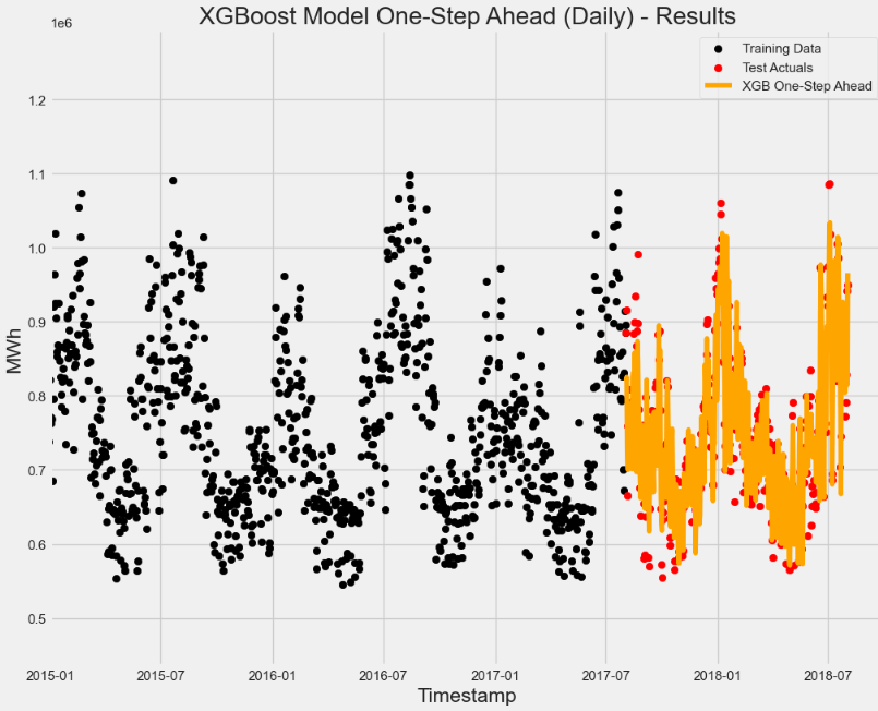
# Let's visually see the results
plt.scatter(x=train.index, y=train['PJME_MW'], label='Training Data', color='black')
plt.scatter(x=test.index, y=test['PJME_MW'], label='Test Actuals', color='red')
plt.plot(XGB_prediction_no_lag, label='XGB No Lag', color='orange')

# Plot Labels, Legends etc
plt.xlabel("Timestamp")
plt.ylabel("MWh")
plt.legend(loc='best')
plt.title('XGBoost Model (Daily) - Results')

# For clarify, let's limit to only 2015 onwards
plt.xlim(datetime(2015, 1, 1),datetime(2018, 10, 1))

plt.show()
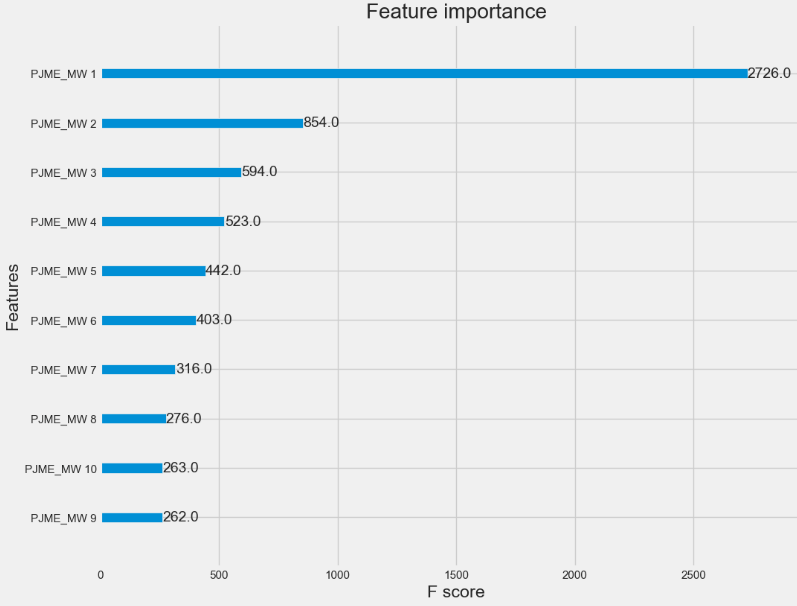
Let’s compare feature importance factors
import xgboost as xgb

xgb.plot_importance(model, max_num_features=10, importance_type='weight') # "weight” is the number of times a feature appears in a tree

plt.show()
from sklearn.metrics import mean_absolute_error

print("MAE XGB: {:.20f}".format(mean_absolute_error(test_label, XGB_prediction['PJME_MW Prediction'])))
MAE XGB: 43437.22089041095750872046
FB Prophet TSF
Let’s look at TSF with FB Prophet using the PJME_hourly.csv dataset
import numpy as np
import pandas as pd
import seaborn as sns
import matplotlib.pyplot as plt
from prophet import Prophet
from sklearn.metrics import mean_squared_error, mean_absolute_error
plt.style.use('fivethirtyeight') # For plots
pjme = pd.read_csv('PJME_hourly.csv',
                   index_col=[0], parse_dates=[0])
# Color pallete for plotting
color_pal = ["#F8766D", "#D39200", "#93AA00",
             "#00BA38", "#00C19F", "#00B9E3",
             "#619CFF", "#DB72FB"]
pjme.plot(style='.', figsize=(15,5), color=color_pal[0], title='PJM East')
plt.show()

Let’s create the features and target variables
def create_features(df, label=None):
    """
    Creates time series features from datetime index.
    """
    df = df.copy()
    df['date'] = df.index
    df['hour'] = df['date'].dt.hour
    df['dayofweek'] = df['date'].dt.dayofweek
    df['quarter'] = df['date'].dt.quarter
    df['month'] = df['date'].dt.month
    df['year'] = df['date'].dt.year
    df['dayofyear'] = df['date'].dt.dayofyear
    df['dayofmonth'] = df['date'].dt.day
    df['weekofyear'] = df['date'].dt.weekofyear

    X = df[['hour','dayofweek','quarter','month','year',
           'dayofyear','dayofmonth','weekofyear']]
    if label:
        y = df[label]
        return X, y
    return X

X, y = create_features(pjme, label='PJME_MW')

features_and_target = pd.concat([X, y], axis=1)
# See our features and target
features_and_target.head()
Let’s split our data into the training and testing sets
split_date = '01-Jan-2015'
pjme_train = pjme.loc[pjme.index <= split_date].copy()
pjme_test = pjme.loc[pjme.index > split_date].copy()
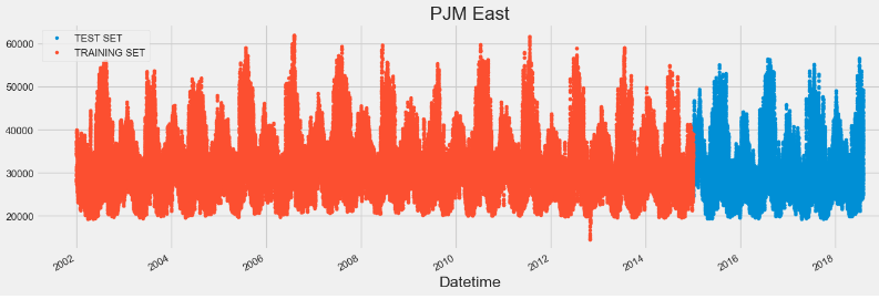
# Plot train and test so you can see where we have split
pjme_test \
    .rename(columns={'PJME_MW': 'TEST SET'}) \
    .join(pjme_train.rename(columns={'PJME_MW': 'TRAINING SET'}),
          how='outer') \
    .plot(figsize=(15,5), title='PJM East', style='.')
plt.show()
# Format data for Prophet model using ds and y
pjme_train.reset_index() \
    .rename(columns={'Datetime':'ds',
                     'PJME_MW':'y'}).head()

# Setup and train model and fit
model = Prophet()
model.fit(pjme_train.reset_index() \
.rename(columns={'Datetime':'ds',
'PJME_MW':'y'}))
# Predict on training set with model
pjme_test_fcst = model.predict(df=pjme_test.reset_index() \
.rename(columns={'Datetime':'ds'}))
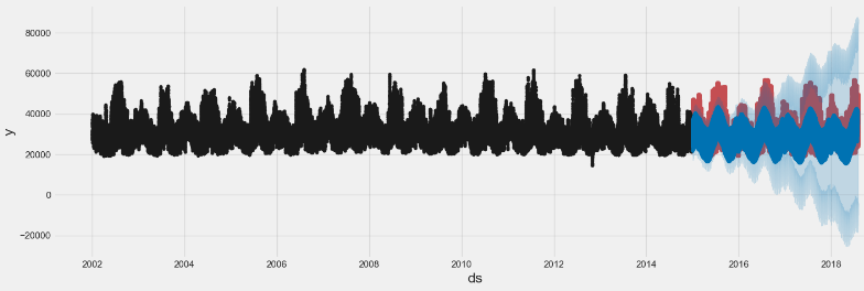
# Plot the forecast
f, ax = plt.subplots(1)
f.set_figheight(5)
f.set_figwidth(15)
fig = model.plot(pjme_test_fcst,
ax=ax)
plt.show()
# Plot the components of the model
fig = model.plot_components(pjme_test_fcst)


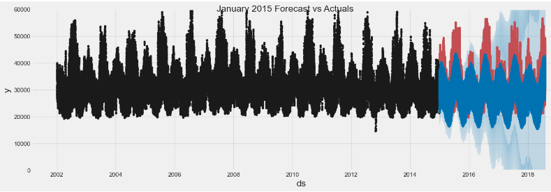
# Plot the forecast with the actuals
f, ax = plt.subplots(1)
f.set_figheight(5)
f.set_figwidth(15)
ax.plot(pjme_test['PJME_MW'], color='r')
fig = model.plot(pjme_test_fcst, ax=ax)
#ax.set_xbound(lower='01-01-2015',
#              upper='02-01-2015')
ax.set_ylim(0, 60000)
plot = plt.suptitle('January 2015 Forecast vs Actuals')
Let’s look at the TSF QC metrics below
mean_squared_error(y_true=pjme_test['PJME_MW'],
                   y_pred=pjme_test_fcst['yhat'])
43759030.158367276
mean_absolute_error(y_true=pjme_test['PJME_MW'],
                   y_pred=pjme_test_fcst['yhat'])
5181.336843800633
def mean_absolute_percentage_error(y_true, y_pred):
    """Calculates MAPE given y_true and y_pred"""
    y_true, y_pred = np.array(y_true), np.array(y_pred)
    return np.mean(np.abs((y_true - y_pred) / y_true)) * 100

mean_absolute_percentage_error(y_true=pjme_test['PJME_MW'],
                   y_pred=pjme_test_fcst['yhat'])
16.514368729991826
Let’s incorporate the US holidays into our forecast
from pandas.tseries.holiday import USFederalHolidayCalendar as calendar

cal = calendar()
train_holidays = cal.holidays(start=pjme_train.index.min(),
                              end=pjme_train.index.max())
test_holidays = cal.holidays(start=pjme_test.index.min(),
                             end=pjme_test.index.max())
# Create a dataframe with holiday, ds columns
pjme['date'] = pjme.index.date
pjme['is_holiday'] = pjme.date.isin([d.date() for d in cal.holidays()])
holiday_df = pjme.loc[pjme['is_holiday']] \
.reset_index() \
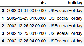
.rename(columns={'Datetime':'ds'})
holiday_df['holiday'] = 'USFederalHoliday'
holiday_df = holiday_df.drop(['PJME_MW','date','is_holiday'], axis=1)
holiday_df.head()
holiday_df['ds'] = pd.to_datetime(holiday_df['ds'])
# Setup and train model with holidays
model_with_holidays = Prophet(holidays=holiday_df)
model_with_holidays.fit(pjme_train.reset_index() \
                            .rename(columns={'Datetime':'ds',
                                             'PJME_MW':'y'}))
# Predict on training set with model
pjme_test_fcst_with_hols = \
    model_with_holidays.predict(df=pjme_test.reset_index() \
                                    .rename(columns={'Datetime':'ds'}))
fig2 = model_with_holidays.plot_components(pjme_test_fcst_with_hols)


Let’s calculate the TSF QC metrics below
mean_squared_error(y_true=pjme_test['PJME_MW'],
                   y_pred=pjme_test_fcst_with_hols['yhat'])
43869232.83337779
mean_absolute_error(y_true=pjme_test['PJME_MW'],
                   y_pred=pjme_test_fcst_with_hols['yhat'])
5189.301126557125
def mean_absolute_percentage_error(y_true, y_pred):
    """Calculates MAPE given y_true and y_pred"""
    y_true, y_pred = np.array(y_true), np.array(y_pred)
    return np.mean(np.abs((y_true - y_pred) / y_true)) * 100

mean_absolute_percentage_error(y_true=pjme_test['PJME_MW'],
                   y_pred=pjme_test_fcst_with_hols['yhat'])
16.54566224842299
Let’s select the summer holiday season 20160407
jul4_test = pjme_test.query('Datetime >= 20160407 and Datetime < 20160408')
jul4_pred = pjme_test_fcst.query('ds >= 20160407 and ds < 20160408')
jul4_pred_holiday_model = pjme_test_fcst_with_hols.query('ds >= 20160407 and ds < 20160408')
mean_absolute_error(y_true=jul4_test['PJME_MW'],
                   y_pred=jul4_pred['yhat'])
2159.482877231659
mean_absolute_error(y_true=jul4_test['PJME_MW'],
                   y_pred=jul4_pred_holiday_model['yhat'])
2158.105151601811
holiday_list = holiday_df['ds'].tolist()
hols_test = pjme_test.query('Datetime in @holiday_list')
hols_pred = pjme_test_fcst.query('ds in @holiday_list')
hols_pred_holiday_model = pjme_test_fcst_with_hols.query('ds in @holiday_list')
mean_absolute_error(y_true=hols_test['PJME_MW'],
                   y_pred=hols_pred['yhat'])
5221.376549904179
mean_absolute_error(y_true=hols_test['PJME_MW'],
                   y_pred=hols_pred_holiday_model['yhat'])
5110.9406084975535
Let’s compare TSF with/without holidays 2015-2018 in terms of MAE
holiday_df['date'] = holiday_df['ds'].dt.date

for hol, d in holiday_df.groupby('date'):
    holiday_list = d['ds'].tolist()
    hols_test = pjme_test.query('Datetime in @holiday_list')
    if len(hols_test) == 0:
        continue
    hols_pred = pjme_test_fcst.query('ds in @holiday_list')
    hols_pred_holiday_model = pjme_test_fcst_with_hols.query('ds in @holiday_list')
    non_hol_error = mean_absolute_error(y_true=hols_test['PJME_MW'],
                   y_pred=hols_pred['yhat'])
    hol_model_error = mean_absolute_error(y_true=hols_test['PJME_MW'],
                       y_pred=hols_pred_holiday_model['yhat'])
    diff = non_hol_error - hol_model_error
    print(f'Holiday: {hol:%B %d, %Y}:    \n MAE (non-holiday model): {non_hol_error:0.1f} \n MAE (Holiday Model): {hol_model_error:0.1f} \n Diff {diff:0.1f}')
Holiday: January 01, 2015:
 MAE (non-holiday model): 3087.8
 MAE (Holiday Model): 2671.8
 Diff 416.1
Holiday: January 19, 2015:
 MAE (non-holiday model): 2410.3
 MAE (Holiday Model): 2088.3
 Diff 322.0
Holiday: February 16, 2015:
 MAE (non-holiday model): 11124.3
 MAE (Holiday Model): 12769.0
 Diff -1644.7
Holiday: May 25, 2015:
 MAE (non-holiday model): 1564.2
 MAE (Holiday Model): 1616.3
 Diff -52.1
Holiday: July 03, 2015:
 MAE (non-holiday model): 6069.5
 MAE (Holiday Model): 4309.8
 Diff 1759.6
Holiday: September 07, 2015:
 MAE (non-holiday model): 3851.9
 MAE (Holiday Model): 4314.2
 Diff -462.3
Holiday: October 12, 2015:
 MAE (non-holiday model): 1594.6
 MAE (Holiday Model): 1873.9
 Diff -279.3
Holiday: November 11, 2015:
 MAE (non-holiday model): 2057.5
 MAE (Holiday Model): 1586.3
 Diff 471.2
Holiday: November 26, 2015:
 MAE (non-holiday model): 4675.9
 MAE (Holiday Model): 3785.6
 Diff 890.3
Holiday: December 25, 2015:
 MAE (non-holiday model): 7566.6
 MAE (Holiday Model): 5883.2
 Diff 1683.4
Holiday: January 01, 2016:
 MAE (non-holiday model): 3804.8
 MAE (Holiday Model): 2254.8
 Diff 1550.0
Holiday: January 18, 2016:
 MAE (non-holiday model): 3317.8
 MAE (Holiday Model): 4779.1
 Diff -1461.3
Holiday: February 15, 2016:
 MAE (non-holiday model): 6876.0
 MAE (Holiday Model): 8513.7
 Diff -1637.6
Holiday: May 30, 2016:
 MAE (non-holiday model): 1737.4
 MAE (Holiday Model): 3103.2
 Diff -1365.8
Holiday: July 04, 2016:
 MAE (non-holiday model): 7406.7
 MAE (Holiday Model): 5788.5
 Diff 1618.2
Holiday: September 05, 2016:
 MAE (non-holiday model): 3057.9
 MAE (Holiday Model): 2093.6
 Diff 964.3
Holiday: October 10, 2016:
 MAE (non-holiday model): 2185.3
 MAE (Holiday Model): 1855.3
 Diff 330.0
Holiday: November 11, 2016:
 MAE (non-holiday model): 2061.5
 MAE (Holiday Model): 1681.7
 Diff 379.8
Holiday: November 24, 2016:
 MAE (non-holiday model): 3508.4
 MAE (Holiday Model): 2700.4
 Diff 808.0
Holiday: December 26, 2016:
 MAE (non-holiday model): 2254.0
 MAE (Holiday Model): 1951.0
 Diff 303.0
Holiday: January 02, 2017:
 MAE (non-holiday model): 1743.7
 MAE (Holiday Model): 1549.9
 Diff 193.8
Holiday: January 16, 2017:
 MAE (non-holiday model): 3049.7
 MAE (Holiday Model): 2872.2
 Diff 177.5
Holiday: February 20, 2017:
 MAE (non-holiday model): 4985.0
 MAE (Holiday Model): 3706.7
 Diff 1278.3
Holiday: May 29, 2017:
 MAE (non-holiday model): 4584.2
 MAE (Holiday Model): 3025.2
 Diff 1558.9
Holiday: July 04, 2017:
 MAE (non-holiday model): 2808.4
 MAE (Holiday Model): 2163.1
 Diff 645.4
Holiday: September 04, 2017:
 MAE (non-holiday model): 5181.2
 MAE (Holiday Model): 3576.4
 Diff 1604.8
Holiday: October 09, 2017:
 MAE (non-holiday model): 7627.9
 MAE (Holiday Model): 9231.5
 Diff -1603.6
Holiday: November 10, 2017:
 MAE (non-holiday model): 2346.6
 MAE (Holiday Model): 3865.4
 Diff -1518.9
Holiday: November 23, 2017:
 MAE (non-holiday model): 3048.2
 MAE (Holiday Model): 2846.6
 Diff 201.6
Holiday: December 25, 2017:
 MAE (non-holiday model): 2004.7
 MAE (Holiday Model): 1693.3
 Diff 311.3
Holiday: January 01, 2018:
 MAE (non-holiday model): 9331.7
 MAE (Holiday Model): 10818.8
 Diff -1487.1
Holiday: January 15, 2018:
 MAE (non-holiday model): 6174.2
 MAE (Holiday Model): 7804.1
 Diff -1629.9
Holiday: February 19, 2018:
 MAE (non-holiday model): 2667.6
 MAE (Holiday Model): 2616.5
 Diff 51.2
Holiday: May 28, 2018:
 MAE (non-holiday model): 3094.5
 MAE (Holiday Model): 2084.5
 Diff 1010.0
Holiday: July 04, 2018:
 MAE (non-holiday model): 3672.4
 MAE (Holiday Model): 5369.3
 Diff -1696.9
The final yhat plot PJME_MW Forecast vs Actuals is
ax = pjme_test_fcst.set_index('ds')['yhat'].plot(figsize=(15, 5),
                                                 lw=0,
                                                 style='.')
pjme_test['PJME_MW'].plot(ax=ax,
                          style='.',
                          lw=0,
                          alpha=0.2)
plt.legend(['Forecast','Actual'])
plt.title('Forecast vs Actuals')
plt.show()

DOM Data
#choosing DOM_hourly.csv data for analysis
fpath='DOM_hourly.csv'

#Let's use datetime(2012-10-01 12:00:00,...) as index instead of numbers(0,1,...)
#This will be helpful for further data analysis as we are dealing with time series data
df = pd.read_csv(fpath, index_col='Datetime', parse_dates=['Datetime'])
df.head()

#checking missing data
df.isna().sum()

#Data visualization

df.plot(figsize=(16,4),legend=True)

plt.title('DOM hourly power consumption data - BEFORE NORMALIZATION')

plt.show()

#Normalize DOM hourly power consumption data
def normalize_data(df):
scaler = sklearn.preprocessing.MinMaxScaler()
df['DOM_MW']=scaler.fit_transform(df['DOM_MW'].values.reshape(-1,1))
return df
df_norm = normalize_data(df)
df_norm.shape
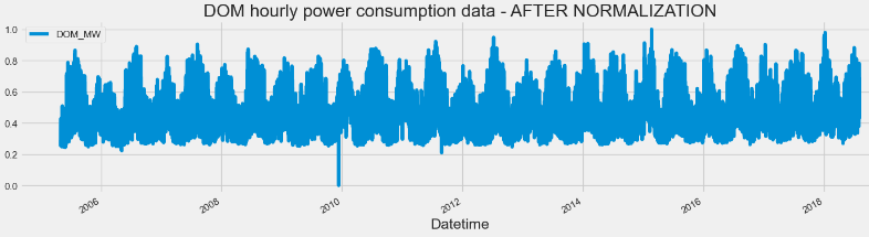
#Visualize data after normalization
df_norm.plot(figsize=(16,4),legend=True)
plt.title('DOM hourly power consumption data - AFTER NORMALIZATION')
plt.show()
RNN TSF
# train data for deep learning models

def load_data(stock, seq_len):
    X_train = []
    y_train = []
    for i in range(seq_len, len(stock)):
        X_train.append(stock.iloc[i - seq_len: i, 0])
        y_train.append(stock.iloc[i, 0])

    # 1 last 6189 days are going to be used in test
    X_test = X_train[110000:]
    y_test = y_train[110000:]

    # 2 first 110000 days are going to be used in training
    X_train = X_train[:110000]
    y_train = y_train[:110000]

    # 3 convert to numpy array
    X_train = np.array(X_train)
    y_train = np.array(y_train)

    X_test = np.array(X_test)
    y_test = np.array(y_test)

    # 4 reshape data to input into RNN models
    X_train = np.reshape(X_train, (110000, seq_len, 1))

    X_test = np.reshape(X_test, (X_test.shape[0], seq_len, 1))

    return [X_train, y_train, X_test, y_test]
#create train, test data
seq_len = 20 #choose sequence length

X_train, y_train, X_test, y_test = load_data(df, seq_len)

print('X_train.shape = ',X_train.shape)
print('y_train.shape = ', y_train.shape)
print('X_test.shape = ', X_test.shape)
print('y_test.shape = ',y_test.shape)
X_train.shape =  (110000, 20, 1)
y_train.shape =  (110000,)
X_test.shape =  (6169, 20, 1)
y_test.shape =  (6169,)
#RNN model
rnn_model = Sequential()
rnn_model.add(SimpleRNN(40,activation="tanh",return_sequences=True, input_shape=(X_train.shape[1],1)))
rnn_model.add(Dropout(0.15))
rnn_model.add(SimpleRNN(40,activation="tanh",return_sequences=True))
rnn_model.add(Dropout(0.15))
rnn_model.add(SimpleRNN(40,activation="tanh",return_sequences=False))
rnn_model.add(Dropout(0.15))
rnn_model.add(Dense(1))
rnn_model.summary()
rnn_model.compile(optimizer="adam",loss="MSE")
rnn_model.fit(X_train, y_train, epochs=10, batch_size=1000)
Model: "sequential_1"
_________________________________________________________________
 Layer (type)                Output Shape              Param #
=================================================================
 simple_rnn (SimpleRNN)      (None, 20, 40)            1680

 dropout_1 (Dropout)         (None, 20, 40)            0

 simple_rnn_1 (SimpleRNN)    (None, 20, 40)            3240

 dropout_2 (Dropout)         (None, 20, 40)            0

 simple_rnn_2 (SimpleRNN)    (None, 40)                3240

 dropout_3 (Dropout)         (None, 40)                0

 dense_1 (Dense)             (None, 1)                 41

=================================================================
Total params: 8,201
Trainable params: 8,201
Non-trainable params: 0
_________________________________________________________________
Epoch 1/10
110/110 [==============================] - 6s 43ms/step - loss: 0.1426
Epoch 2/10
110/110 [==============================] - 5s 45ms/step - loss: 0.0329
Epoch 3/10
110/110 [==============================] - 5s 44ms/step - loss: 0.0188
Epoch 4/10
110/110 [==============================] - 5s 46ms/step - loss: 0.0124
Epoch 5/10
110/110 [==============================] - 5s 48ms/step - loss: 0.0094
Epoch 6/10
110/110 [==============================] - 5s 48ms/step - loss: 0.0075
Epoch 7/10
110/110 [==============================] - 5s 46ms/step - loss: 0.0063
Epoch 8/10
110/110 [==============================] - 5s 48ms/step - loss: 0.0055
Epoch 9/10
110/110 [==============================] - 5s 48ms/step - loss: 0.0048
Epoch 10/10
110/110 [==============================] - 5s 45ms/step - loss: 0.0043
#r2 score for the values predicted by the above trained SIMPLE RNN model

rnn_predictions = rnn_model.predict(X_test)
rnn_score = r2_score(y_test,rnn_predictions)
print("R2 Score of RNN model = ",rnn_score)
193/193 [==============================] - 1s 2ms/step
R2 Score of RNN model =  0.9336592349434713
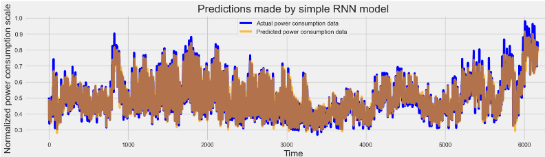
# compare the actual values vs predicted values by plotting a graph

def plot_predictions(test, predicted, title):
    plt.figure(figsize=(16, 4))
    plt.plot(test, color='blue', label='Actual power consumption data')
    plt.plot(predicted, alpha=0.7, color='orange', label='Predicted power consumption data')
    plt.title(title)
    plt.xlabel('Time')
    plt.ylabel('Normalized power consumption scale')
    plt.legend()
    plt.show()
plot_predictions(y_test, rnn_predictions, "Predictions made by simple RNN model")
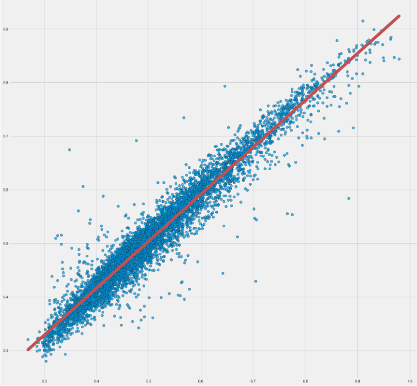
# Initialize layout
x=y_test
y=rnn_predictions
fig, ax = plt.subplots(figsize = (19, 19))
# Add scatterplot
ax.scatter(x, y, s=60, alpha=0.7, edgecolors="k")
b, a = np.polyfit(x, y, deg=1)

# Plot regression line
ax.plot(x, a + b * x, color="r", lw=8.5);
Let’s look at the x=y_test vs y=rnn_predictions scatter plot and the linear regression fit (red line):
LSTM TSF
#train model for LSTM

lstm_model = Sequential()
lstm_model.add(LSTM(40,activation="tanh",return_sequences=True, input_shape=(X_train.shape[1],1)))
lstm_model.add(Dropout(0.15))
lstm_model.add(LSTM(40,activation="tanh",return_sequences=True))
lstm_model.add(Dropout(0.15))
lstm_model.add(LSTM(40,activation="tanh",return_sequences=False))
lstm_model.add(Dropout(0.15))
lstm_model.add(Dense(1))
lstm_model.summary()
lstm_model.compile(optimizer="adam",loss="MSE")
lstm_model.fit(X_train, y_train, epochs=10, batch_size=1000)
Model: "sequential_2"
_________________________________________________________________
 Layer (type)                Output Shape              Param #
=================================================================
 lstm_1 (LSTM)               (None, 20, 40)            6720

 dropout_4 (Dropout)         (None, 20, 40)            0

 lstm_2 (LSTM)               (None, 20, 40)            12960

 dropout_5 (Dropout)         (None, 20, 40)            0

 lstm_3 (LSTM)               (None, 40)                12960

 dropout_6 (Dropout)         (None, 40)                0

 dense_2 (Dense)             (None, 1)                 41

=================================================================
Total params: 32,681
Trainable params: 32,681
Non-trainable params: 0
_________________________________________________________________
Epoch 1/10
110/110 [==============================] - 19s 140ms/step - loss: 0.0214
Epoch 2/10
110/110 [==============================] - 17s 157ms/step - loss: 0.0121
Epoch 3/10
110/110 [==============================] - 18s 163ms/step - loss: 0.0087
Epoch 4/10
110/110 [==============================] - 19s 172ms/step - loss: 0.0050
Epoch 5/10
110/110 [==============================] - 18s 168ms/step - loss: 0.0037
Epoch 6/10
110/110 [==============================] - 19s 172ms/step - loss: 0.0027
Epoch 7/10
110/110 [==============================] - 19s 176ms/step - loss: 0.0023
Epoch 8/10
110/110 [==============================] - 18s 167ms/step - loss: 0.0020
Epoch 9/10
110/110 [==============================] - 19s 170ms/step - loss: 0.0018
Epoch 10/10
110/110 [==============================] - 19s 175ms/step - loss: 0.0017
#r2 score for the values predicted by the above trained LSTM model
lstm_predictions = lstm_model.predict(X_test)
lstm_score = r2_score(y_test, lstm_predictions)
print("R^2 Score of LSTM model = ",lstm_score)
193/193 [==============================] - 2s 5ms/step
R^2 Score of LSTM model =  0.9544869239205461
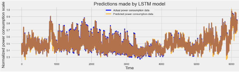
#actual values vs predicted values by plotting a graph
plot_predictions(y_test, lstm_predictions, "Predictions made by LSTM model")
# Initialize layout
x=y_test
y=lstm_predictions
fig, ax = plt.subplots(figsize = (19, 19))
# Add scatterplot
ax.scatter(x, y, s=60, alpha=0.7, edgecolors="k")
b, a = np.polyfit(x, y, deg=1)

# Plot regression line
ax.plot(x, a + b * x, color="r", lw=8.5);
Let’s look at the x=y_test vs y=lstm_predictions scatter plot and the linear regression fit (red line):

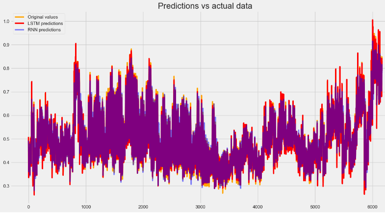
#RNN, LSTM model by plotting data in a single graph
plt.figure(figsize=(15,8))
plt.plot(y_test, c="orange", linewidth=3, label="Original values")
plt.plot(lstm_predictions, c="red", linewidth=3, label="LSTM predictions")
plt.plot(rnn_predictions, alpha=0.5, c="blue", linewidth=3, label="RNN predictions")
plt.legend()
plt.title("Predictions vs actual data", fontsize=20)
plt.show()
plt.figure(figsize=(15,8))
plt.scatter(y_test,lstm_predictions,c="blue", label="LSTM predictions")
plt.scatter(y_test,rnn_predictions,c="k", label="RNN predictions")
plt.scatter(y_test,y_test,c="r", label="Ideal Fit")
plt.legend(["LSTM predictions" , "RNN predictions",'Ideal predictions'])

AEP Data
Let’s import the key libraries
#mathematical operations
import math
import scipy as sp
import numpy as np

#data handling
import pandas as pd

#plotting
import matplotlib as mpl
import matplotlib.pyplot as plt
from statsmodels.graphics.tsaplots import plot_acf
from statsmodels.graphics.tsaplots import plot_pacf
import seaborn as sns
sns.set()

#machine learning and statistical methods
import statsmodels.api as sm

#dataframe index manipulations
import datetime

#selected preprocessing and evaluation methods
from sklearn.preprocessing import StandardScaler
from statsmodels.tsa.stattools import kpss
from sklearn.metrics import mean_absolute_error
from sklearn.metrics import mean_squared_error

#muting unnecessary warnings if needed
import warnings
and load the AEP data
#loading raw data
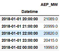
df_aep = pd.read_csv("AEP_hourly.csv", index_col=0)
df_aep.tail()
#sorting unordered indices
df_aep.sort_index(inplace = True)
#visual checking of data. Plotting by Pandas method, drawing axes by Matplotlib
import matplotlib
matplotlib.rc('xtick', labelsize=16)
matplotlib.rc('ytick', labelsize=16)
f, ax = plt.subplots(figsize=(16,6),dpi=200);
plt.suptitle('American Electric Power (AEP) estimated energy consumption in MegaWatts (MW)', fontsize=24);
df_aep.plot(ax=ax,rot=90,ylabel='MW');
plt.xlabel('Date-Time', fontsize=20)
plt.ylabel('MW', fontsize=20)

Data preparations:
#creating datetime list with boundaries of raw data series, hourly frequency
datelist = pd.date_range(datetime.datetime(2004,10,1,1,0,0), datetime.datetime(2018,8,3,0,0,0), freq='H').tolist()

#extracting raw data series indices
idx_list = df_aep.index.to_list()

#checking for anomalies by comparing the two
idx_list == datelist
False
#converting dataframe indices to datetime
dt_idc = pd.to_datetime(df_aep.index, format='%Y-%m-%d %H:%M:%S')
#changing string indices to datetime converted indices
df_aep.set_index(dt_idc, inplace=True)
#collecting important values of irregular indices (index value and timedelta) for later use
idc = []

#iterating through datetime indices
for idx in range(1,len(dt_idc)):

    #if statement is True, if difference between consecutive datetime indices is not one hour
    if dt_idc[idx] - dt_idc[idx-1] != datetime.timedelta(hours=1):

        #appending collection of important values
        idc.append([idx,dt_idc[idx] - dt_idc[idx-1]])
#changing string indices to datetime converted indices
df_aep.set_index(dt_idc, inplace=True)
#correction of anomalies in reversed order avoiding index shift
for idx in reversed(idc):

    #appending mean values in case of datetime gaps
    if idx[1] == datetime.timedelta(hours=2):
        idx_old = df_aep.iloc[idx[0]].name
        idx_new = idx_old-datetime.timedelta(hours=1)
        df_aep.loc[idx_new] = np.mean(df_aep.iloc[idx[0]-1:idx[0]+1].values)

    #dropping duplicates, appending mean of dropped values
    elif idx[1] == datetime.timedelta(hours=0):
        idx_old = df_aep.iloc[idx[0]].name
        value = np.mean(df_aep.iloc[idx[0]-1:idx[0]+1].values)
        df_aep.drop(df_aep.iloc[idx[0]-1:idx[0]+1].index, inplace=True)
        df_aep.loc[idx_old] = value
df_aep.sort_index(inplace=True)
#checking for datetime series again
idx_list = df_aep.index.to_list()
idx_list == datelist
True
#setting frequency attribute of datetime index
df_aep.index.freq = 'H'
Multi-Seasonal TSF
# Decomposition of time series to individual components
#splitting time series to train and test sub series (test series of one year)
y_train = df_aep.iloc[:-8766,:]
y_test = df_aep.iloc[-8766:,:]

#extracting daily seasonality from raw time series
sd_24 = sm.tsa.seasonal_decompose(y_train, period=24)

#extracting weekly seasonality from time series adjusted by daily seasonality
sd_168 = sm.tsa.seasonal_decompose(y_train - np.array(sd_24.seasonal).reshape(-1,1), period=168)

#extracting yearly seasonality from time series adjusted by daily and weekly seasonality
sd_8766 = sm.tsa.seasonal_decompose(y_train - np.array(sd_168.seasonal).reshape(-1,1), period=8766)
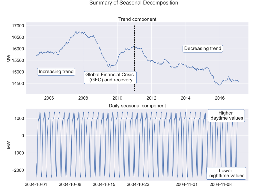
#drawing figure with subplots, predefined size and resolution
f, axes = plt.subplots(5,1,figsize=(18,34),dpi=200);
#setting figure title and adjusting title position and size
plt.suptitle('Summary of Seasonal Decomposition', y=0.92, fontsize=24);
#plotting trend component
axes[0].plot(sd_8766.trend)
axes[0].set_title('Trend component', fontdict={'fontsize': 22});
#drawing black dashed vertical lines between y axis limits
axes[0].vlines(datetime.datetime(2008,1,1), axes[0].get_ylim()[0], axes[0].get_ylim()[1], colors='black', linestyles='dashed');
axes[0].vlines(datetime.datetime(2011,1,1), axes[0].get_ylim()[0], axes[0].get_ylim()[1], colors='black', linestyles='dashed');
#placing three comments in text boxes
axes[0].text(datetime.datetime(2006,6,1), 15000, 'Increasing trend',
ha='center', va='center', bbox=dict(fc='white', ec='b', boxstyle='round'));
axes[0].text(datetime.datetime(2009,8,1), 14750, 'Global Financial Crisis \n (GFC) and recovery',
ha='center', va='center', bbox=dict(fc='white', ec='b', boxstyle='round'));
axes[0].text(datetime.datetime(2015,1,1), 16000, 'Decreasing trend',
ha='center', va='center', bbox=dict(fc='white', ec='b', boxstyle='round'));
#plotting daily seasonal component
axes[1].plot(sd_24.seasonal[:1000]);
axes[1].set_title('Daily seasonal component', fontdict={'fontsize': 22});
axes[1].annotate('Higher \n daytime values', xy=(0.54, 0.50),
xycoords='axes fraction',
va='center', ha='center',
xytext=(0.9, 0.9),
textcoords='axes fraction',
bbox=dict(boxstyle='round', fc='w', ec='b'));
axes[1].annotate('Lower \n nighttime values', xy=(0.54, 0.50),
xycoords='axes fraction',
va='center', ha='center',
xytext=(0.9, 0.1),
textcoords='axes fraction',
bbox=dict(boxstyle='round', fc='w', ec='b'));
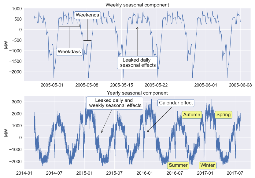
#plotting weekly seasonal component
axes[2].plot(sd_168.seasonal[5000:6000]);
axes[2].set_title('Weekly seasonal component', fontdict={'fontsize': 22});
#placing comment in annotation with text box and arrow
axes[2].annotate('Leaked daily \n seasonal effects', xy=(0.50, 0.75),
xycoords='axes fraction',
va='center', ha='center',
xytext=(0.50, 0.25),
textcoords='axes fraction',
bbox=dict(boxstyle='round', fc='w', ec='b'),
arrowprops=dict(color='black',
arrowstyle='->',
connectionstyle='arc3'));
axes[2].annotate('Weekdays', xy=(0.20, 0.75),
xycoords='axes fraction',
va='center', ha='center',
xytext=(0.20, 0.40),
textcoords='axes fraction',
bbox=dict(boxstyle='round', fc='w', ec='b'),
arrowprops=dict(color='black',
arrowstyle='-[',
mutation_scale=45,
connectionstyle='arc3'));
axes[2].annotate('Weekends', xy=(0.28, 0.55),
xycoords='axes fraction',
va='center', ha='center',
xytext=(0.28, 0.90),
textcoords='axes fraction',
bbox=dict(boxstyle='round', fc='w', ec='b'),
arrowprops=dict(color='black',
arrowstyle='-[',
mutation_scale=17,
connectionstyle='arc3'));
#plotting yearly seasonality
axes[3].plot(sd_8766.seasonal[-30000:]);
axes[3].set_title('Yearly seasonal component', fontdict={'fontsize': 22});
#placing comments in annotations with text boxes and arrows
axes[3].annotate('Calendar effect', xy=(0.54, 0.50),
xycoords='axes fraction',
va='center', ha='center',
xytext=(0.67, 0.9),
textcoords='axes fraction',
bbox=dict(boxstyle='round', fc='w', ec='b'),
arrowprops=dict(color='black',
arrowstyle='->',
connectionstyle='arc3'));
axes[3].annotate('Leaked daily and \n weekly seasonal effects', xy=(0.34, 0.49),
xycoords='axes fraction',
va='center', ha='center',
xytext=(0.40, 0.90),
textcoords='axes fraction',
bbox=dict(boxstyle='round', fc='w', ec='b'),
arrowprops=dict(color='black',
arrowstyle='->',
connectionstyle='arc3'));
axes[3].annotate('Summer', xy=(0.54, 0.50),
xycoords='axes fraction',
va='center', ha='center',
xytext=(0.68, 0.05),
textcoords='axes fraction',
bbox=dict(boxstyle='round', fc='#f5f88f', ec='b'));
axes[3].annotate('Autumn', xy=(0.54, 0.50),
xycoords='axes fraction',
va='center', ha='center',
xytext=(0.74, 0.74),
textcoords='axes fraction',
bbox=dict(boxstyle='round', fc='#f5f88f', ec='b'));
axes[3].annotate('Winter', xy=(0.54, 0.50),
xycoords='axes fraction',
va='center', ha='center',
xytext=(0.81, 0.05),
textcoords='axes fraction',
bbox=dict(boxstyle='round', fc='#f5f88f', ec='b'));
axes[3].annotate('Spring', xy=(0.54, 0.50),
xycoords='axes fraction',
va='center', ha='center',
xytext=(0.88, 0.74),
textcoords='axes fraction',
bbox=dict(boxstyle='round', fc='#f5f88f', ec='b'));
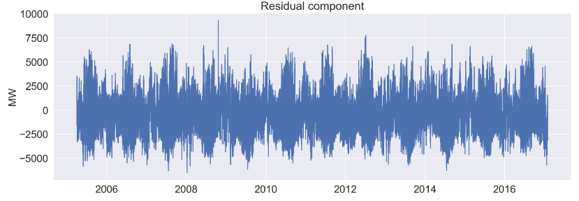
#plotting residual of decomposition
axes[4].plot(sd_8766.resid);
axes[4].set_title('Residual component', fontdict={'fontsize': 22});
#setting label for each y axis
for a in axes:
a.set_ylabel('MW',fontsize=20);
plt.show();
UCM Approximations
# Approximation functions of model components
#selecting datetime indices for approximating the assumed linear decreasing trend with linear model
#selection excludes NaN values introduced by moving average calculation during decomposition
pred_idx_p1 = mpl.dates.date2num(df_aep.iloc[-8766*7-4383:-8766-4383,:].index.values)

#selecting total datetime indices for approximating trend with 3rd degree polynomial model
#selection excludes NaN values introduced by moving average calculation during decomposition
pred_idx_p3 = mpl.dates.date2num(df_aep.iloc[4383:-8766-4383,:].index.values)

#selecting indices for plotting linear and 3rd degree polynomial models respectively
fcast_idx_p1 = mpl.dates.date2num(df_aep.loc[datetime.datetime(2011,1,1):,:].index.values)
fcast_idx_p3 = mpl.dates.date2num(df_aep.loc[datetime.datetime(2006,1,1):,:].index.values)

#fitting models with numpy
poly1 = np.polyfit(pred_idx_p1, sd_8766.trend.values[-8766*6-4383:-4383], 1)
poly3 = np.polyfit(pred_idx_p3, sd_8766.trend.values[4383:-4383], 3)

#Constructing fitted models
fcast_t_p1m = np.poly1d(poly1)
fcast_t_p3m = np.poly1d(poly3)

#In-sample trend prediction of constructed models
fcast_t_p1r = fcast_t_p1m(fcast_idx_p1)
fcast_t_p3r = fcast_t_p3m(fcast_idx_p3)

#drawing figure with predefined size and resolution
plt.figure(figsize=(18,6),dpi=200);

#setting title and size of title
plt.suptitle('Comparison of linear and 3rd degree polynomial models of trend component', fontsize=24);

#setting y axis label
plt.ylabel('MW',fontsize=22);
plt.xlabel('Date',fontsize=22);

#plotting trend component
plt.plot(sd_8766.trend[4383:-4383], label='Trend component',lw=3);

#plotting linear model of trend component
plt.plot(fcast_idx_p1, fcast_t_p1r, label='Linear model',lw=6);

#plotting 3rd degree polynomial model of trend component
plt.plot(fcast_idx_p3, fcast_t_p3r, label='3rd degree polynomial model',lw=3);

plt.legend(fontsize=20);

#generating arrays for mapping current hour of the day, current day of week and
#current day of year to seasonal components, which are to be modeled by trigonometric functions
#the corresponding values determine the current phase and serve as inputs for the trigonometric approximation
idxh = sd_24.seasonal.index.hour
idxw = sd_168.seasonal.index.dayofweek * 24 + idxh
idxd = sd_8766.seasonal.index.dayofyear
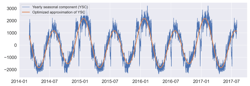
#defining function for approximating yearly seasonal component
#x: datetime, A,C: amplitudes, b,d: phase shifts, E: constant. Periods are predefined
def fy(x, A, b, C, d, E):
return A * np.sin(4*np.pi/365.25 * x + b) + C * np.cos(2*np.pi/365.25 * x + d) + E
#datetime indices are converted to integers for 'fy' approximation function
tidx = mpl.dates.date2num(sd_8766.seasonal.index.values)
#optimizing manual approximation using scipy
params_y, params_y_covariance = sp.optimize.curve_fit(fy, idxd, sd_8766.seasonal, p0=[2300, 0.8, 1000, -0.25, 1])

#printing parameters for yearly seasonal component optimized approximation ('fy')
print(params_y)

#drawing figure with predefined size and resolution
plt.figure(figsize=(18,6),dpi=200);

#plotting arbitrarily selected time window of observed values
plt.plot(sd_8766.seasonal[-30000:], label='Yearly seasonal component (YSC)');

#plotting optimized approximation
plt.plot(sd_8766.seasonal.index[-30000:], fy(tidx, params_y[0],
                                            params_y[1],
                                            params_y[2],
                                            params_y[3],
                                            params_y[4])[-30000:], label='Optimized approximation of YSC',lw=3);
plt.legend(fontsize=16,loc='upper left');
[ 1.66859304e+03 7.99408119e-01 5.27402039e+02 -7.08237362e-02 -7.69602255e-02]
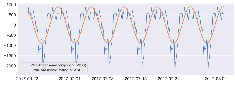
#defining function for approximating weekly seasonal component
#x: datetime, A,C: amplitudes, b,d: phase shifts, E: constant. Periods are predefined
def fw(x, A, b, C, d, E):
    return A * np.sin(2*np.pi/168 * x + b) + C * np.cos(2*np.pi/168 * x + d) + E
#optimizing manual approximation using scipy
params_w, params_w_covariance = sp.optimize.curve_fit(fw, idxw, sd_168.seasonal, p0=[1400, 4, 600, 4, -200])

#printing parameters for weekly seasonal component optimized approximation ('fw')
print(params_w)

plt.figure(figsize=(18,6),dpi=200);

#plotting arbitrarily selected time window of observed values
plt.plot(sd_168.seasonal[-1000:], label='Weekly seasonal component (WSC)');

#plotting optimized approximation
plt.plot(sd_168.seasonal.index[-1000:], fw(idxw, params_w[0],
                                            params_w[1],
                                            params_w[2],
                                            params_w[3],
                                            params_w[4])[-1000:], label='Optimized approximation of WSC',lw=3);
plt.legend(fontsize=16,loc='lower left');
[1.56900789e+03 3.54532262e+00 2.10969647e+03 4.71959966e+00 2.02799797e-02]
#defining function for approximating daily seasonal component
#x: datetime, A,C: amplitudes, b,d: phase shifts, E: constant. Periods are predefined
def fd(x, A, b, C, d, E):
    return A * np.sin(2*np.pi/24 * x + b) + C * np.cos(2*np.pi/24 * x + d) + E
#optimizing manual approximation using scipy
params_d, params_d_covariance = sp.optimize.curve_fit(fd, idxh, sd_24.seasonal, p0=[2300, 5, 1000, 5, 1])

#printing parameters for daily seasonal component optimized approximation ('fd')
print(params_d)

plt.figure(figsize=(18,6),dpi=200);

#plotting arbitrarily selected time window of observed values
plt.plot(sd_24.seasonal[-100:], label='Daily seasonal component (DSC)');

#plotting optimized approximation
plt.plot(sd_24.seasonal.index[-100:], fd(idxh, params_d[0],
                                            params_d[1],
                                            params_d[2],
                                            params_d[3],
                                            params_d[4])[-100:], label='Optimized approximation of DSC',lw=3);
plt.legend(fontsize=16,loc='lower left');
[ 1.68843445e+03 3.66954173e+00 -5.94042160e+00 5.69302202e+00 -5.37078811e-02]

# Component analysis of optimized model
#redifining input values of datetime integers for forecasting trend
idx = mpl.dates.date2num(df_aep.index.values)
#shorthand for dataframe indices
didx = df_aep.index.values
#redefining phase arrays for forecasting
idxh = df_aep.index.hour
idxw = df_aep.index.dayofweek * 24 + idxh
idxd = df_aep.index.dayofyear
#modeled values for each component (sd for seasonal decompose, y: yearly, w: weekly, d: daily, m: model)
trend_m = fcast_t_p3m(idx)
sd_ym = fy(idxd, params_y[0], params_y[1], params_y[2], params_y[3], params_y[4])
sd_wm = fw(idxw, params_w[0], params_w[1], params_w[2], params_w[3], params_w[4])
sd_dm = fd(idxh, params_d[0], params_d[1], params_d[2], params_d[3], params_d[4])
#In-sample prediction of model
sd_full_pred = trend_m[:-8766] + sd_dm[:-8766] + sd_wm[:-8766] + sd_ym[:-8766]
#Out-of-sample prediction (forecast) of model
sd_full_fcast = trend_m[-8766:] + sd_dm[-8766:] + sd_wm[-8766:] + sd_ym[-8766:]
#In-sample prediction residuals
sd_resid_pred = [sd_full_pred[x] - df_aep.iloc[:-8766,:].values[x] for x in range(len(sd_full_pred))]
#Out-of-sample prediction residuals
sd_resid_fcast = [sd_full_fcast[x] - df_aep.iloc[-8766:,:].values[x] for x in range(len(sd_full_fcast))]
#acquiring matplotlib default coloring order to match colors of same component on different plots
prop_cycle = mpl.rcParams['axes.prop_cycle']
colors = prop_cycle.by_key()['color']
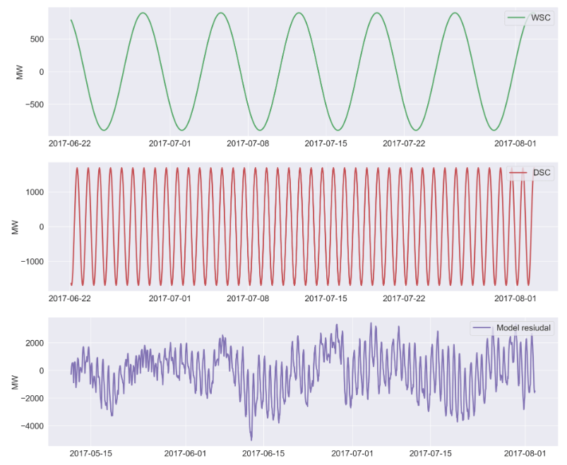
f, axes = plt.subplots(7,1,figsize=(22,46),dpi=200);
plt.suptitle('Component analysis and TSF of optimized model', fontsize=24, y=0.9)
#plotting each component on same subplot. Twin y axis is generated for seasonal components and residual for scaling
axes[0].plot(didx[-9766:-8766], trend_m[-9766:-8766], label='Trend component', color=colors[0],lw=3);
axt = axes[0].twinx();
axt.plot(didx[-9766:-8766], sd_ym[-9766:-8766], label='YSC', color=colors[1],lw=3);
axt.plot(didx[-9766:-8766], sd_wm[-9766:-8766], label='WSC', color=colors[2],lw=3);
axt.plot(didx[-9766:-8766], sd_dm[-9766:-8766], label='DSC', color=colors[3],lw=3);
axt.plot(didx[-9766:-8766], sd_resid_pred[-1000:], label='Model resiudal', color=colors[4],lw=3);
#plotting trend component individually
axes[1].plot(didx[:-8766], trend_m[:-8766], label='Trend component', color=colors[0],lw=3);
#plotting yearly seasonal component individually
axes[2].plot(didx[:-8766], sd_ym[:-8766], label='YSC', color=colors[1],lw=3);
#plotting weekly seasonal component individually (arbitrary time window)
axes[3].plot(didx[-9766:-8766], sd_wm[-9766:-8766], label='WSC', color=colors[2],lw=3);
#plotting daily seasonal component individually (arbitrary time window)
axes[4].plot(didx[-9766:-8766], sd_dm[-9766:-8766], label='DSC', color=colors[3],lw=3);
#plotting residual individually (arbitrary time window)
axes[5].plot(didx[-10766:-8766], sd_resid_pred[-2000:], label='Model resiudal', color=colors[4],lw=3);
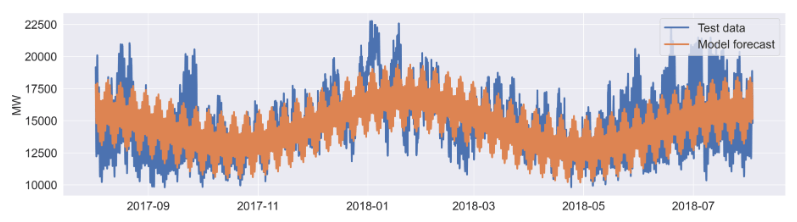
#plotting observed data of test time window
axes[6].plot(df_aep.iloc[-8766:,:], label='Test data',lw=3);
#plotting forecast of test time window
axes[6].plot(didx[-8766:], sd_full_fcast, label='Model forecast',lw=3);
axes[0].legend(loc='upper left',fontsize=20);
axes[0].set_ylabel('MW',fontsize=20);
axt.legend(loc='upper right',fontsize=20);
for a in axes[1:]:
a.set_ylabel('MW',fontsize=20);
a.legend(loc='upper right',fontsize=20);
plt.show();

UCM Residual Diagnostics
#calculating mean absolute error and root mean squared error for model evaluation
MAE_sd = mean_absolute_error(df_aep.iloc[-8766:,0].values, sd_full_fcast)
RMSE_sd = mean_squared_error(df_aep.iloc[-8766:,0].values, sd_full_fcast, squared=False)

print(f'Mean absolute error (MAE): {"%.0f" % MAE_sd}, Root mean squared error (RMSE): {"%.0f" % RMSE_sd}')
Mean absolute error (MAE): 1420, Root mean squared error (RMSE): 1824
#shorthand for observed data of test time window
y_test = df_aep.iloc[-8766:,0].values

#calculating integral for observation function and forecast function (total yearly energy demand in MWh)
observed_integral = np.cumsum([y_test[x] + (y_test[x+1] - y_test[x]) / 2 for x in range(len(y_test)-1)])[-1]
model_sd_integral = np.cumsum([sd_full_fcast[x] + (sd_full_fcast[x+1] - sd_full_fcast[x]) / 2 for x in range(len(sd_full_fcast)-1)])[-1]

#calculating absolute and percentage error of forecast integral compared to observed integral
fcast_integral_abserror = model_sd_integral - observed_integral
fcast_integral_perror_sd = (model_sd_integral - observed_integral) *100 / observed_integral

print(f"Observed yearly energy demand: {'%.3e' % observed_integral} MWh")
print(f"Forecast yearly energy demand: {'%.3e' % model_sd_integral} MWh")
print(f"Forecast error of yearly energy demand: {'%.3e' % fcast_integral_abserror} MWh or {'%.3f' % fcast_integral_perror_sd} %")
Observed yearly energy demand: 1.312e+08 MWh
Forecast yearly energy demand: 1.281e+08 MWh
Forecast error of yearly energy demand: -3.067e+06 MWh or -2.338 %
Unobserved Components Model (UCM)
#splitting time series to train and test subsets
y_train = df_aep.iloc[:-8766,:].copy()
y_test = df_aep.iloc[-8766:,:].copy()

#Unobserved Components model definition
model_UC1 = sm.tsa.UnobservedComponents(y_train,
                                        level='dtrend',
                                        irregular=True,
                                        stochastic_level = False,
                                        stochastic_trend = False,
                                        stochastic_freq_seasonal = [False, False, False],
                                        freq_seasonal=[{'period': 24, 'harmonics': 1},
                                                       {'period': 168, 'harmonics': 1},
                                                       {'period': 8766, 'harmonics': 2}])
#fitting model to train data
model_UC1res = model_UC1.fit()

#printing statsmodels summary for model
print(model_UC1res.summary())

print("")

#calculating mean absolute error and root mean squared error for in-sample prediction of model
print(f"In-sample mean absolute error (MAE): {'%.0f' % model_UC1res.mae}, In-sample root mean squared error (RMSE): {'%.0f' % np.sqrt(model_UC1res.mse)}")

#model forecast
forecast_UC1 = model_UC1res.forecast(steps=8766)

#calculating mean absolute error and root mean squared error for out-of-sample prediction for model evaluation
RMSE_UC1 = np.sqrt(np.mean([(y_test.iloc[x,:] - forecast_UC1[x]) ** 2 for x in range(len(forecast_UC1))]))
MAE_UC1 = np.mean([np.abs(y_test.iloc[x,:] - forecast_UC1[x]) for x in range(len(forecast_UC1))])

print(f"Out-of-sample mean absolute error (MAE): {'%.0f' % MAE_UC1}, Out-of-sample root mean squared error (RMSE): {'%.0f' % RMSE_UC1}")
Unobserved Components Results
====================================================================================
Dep. Variable:                       AEP_MW   No. Observations:               112530
Model:                  deterministic trend   Log Likelihood            -1002257.011
                     + freq_seasonal(24(1))   AIC                        2004516.023
                    + freq_seasonal(168(1))   BIC                        2004525.654
                   + freq_seasonal(8766(2))   HQIC                       2004518.930
Date:                      Thu, 21 Sep 2023
Time:                              14:48:08
Sample:                          10-01-2004
                               - 08-02-2017
Covariance Type:                        opg
====================================================================================
                       coef    std err          z      P>|z|      [0.025      0.975]
------------------------------------------------------------------------------------
sigma2.irregular  3.168e+06    1.3e+04    244.090      0.000    3.14e+06    3.19e+06
===================================================================================
Ljung-Box (L1) (Q):              104573.71   Jarque-Bera (JB):              2731.37
Prob(Q):                              0.00   Prob(JB):                         0.00
Heteroskedasticity (H):               1.04   Skew:                             0.35
Prob(H) (two-sided):                  0.00   Kurtosis:                         3.30
===================================================================================

Warnings:
[1] Covariance matrix calculated using the outer product of gradients (complex-step).

In-sample mean absolute error (MAE): 1424, In-sample root mean squared error (RMSE): 1787
Out-of-sample mean absolute error (MAE): 1420, Out-of-sample root mean squared error (RMSE): 1822
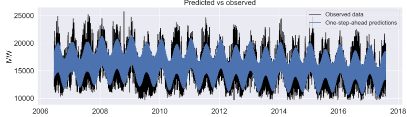
f, axes = plt.subplots(7,1,figsize=(18,40),dpi=200)
#custom plotting of observed train data in style of results class '.plot_components()' method
#plotting observed data vs. in-sample prediction
axes[0].plot(y_train.iloc[15000:,:], label='Observed data', color='black');
axes[0].plot(model_UC1res.fittedvalues.iloc[15000:], label='One-step-ahead predictions');
axes[0].legend(fontsize=16);
#plotting smoothed level component
axes[1].plot(y_train.index, model_UC1res.level['smoothed'], label='Level (smoothed)');
axes[1].legend(fontsize=16);
#plotting smoothed trend component
axes[2].plot(y_train.index, model_UC1res.trend['smoothed'], label='Trend (smoothed)');
axes[2].set_ylim(-1,1)
axes[2].legend(fontsize=16);
limits = [-300, -1200, 0]
#plotting smoothed seasonal components with arbitrary time window scales
for i in range(3,6,1):
axes[i].plot(y_train.index[limits[i-3]:], model_UC1res.freq_seasonal[i-3]['smoothed'][limits[i-3]:], label=model_UC1res.freq_seasonal[i-3]['pretty_name']);
axes[i].legend(loc='upper right');
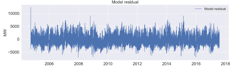
#plotting residuals
axes[6].plot(y_train.index, model_UC1res.resid, label='Model residual');
axes[6].legend(fontsize=16);
#list of subplot titles
axtitles = ['Predicted vs observed',
'Level component',
'Trend component',
model_UC1res.freq_seasonal[0]['pretty_name'],
model_UC1res.freq_seasonal[1]['pretty_name'],
model_UC1res.freq_seasonal[2]['pretty_name'],
'Model residual']
#setting y labels and subplot titles (former is missing from '.plot_components()')
for i,a in enumerate(axes):
a.set_ylabel('MW',fontsize=20)
a.set_title(axtitles[i],fontsize=20)
plt.show();
Let’s skip the auxiliary plots of level, trend, seasonal 24 (1), 168 (1), and 8766 (2).
#Final UCM residual diagnostics
#plotting residual diagnostics of Unobserved Components model
model_UC1res.plot_diagnostics(figsize=(12,12),lags=60).set_dpi(200);
plt.show();


print(f"Point forecast one year ahead: {'%.1f' % forecast_UC1[-1]}, observed value: {y_test.iloc[-1,0]}, relative difference: {'%.2f' % ((forecast_UC1[-1] - y_test.iloc[-1,0]) * 100 / y_test.iloc[-1,0])}%")
Point forecast one year ahead: 15117.5, observed value: 14809.0, relative difference: 2.08%
Summary
- Throughout this study, we have tested and compared several models to forecast monthly electricity consumption from American Electric Power Company (AEP) clients. These models are based solely on time series data.
- Comprehensive QC tests have shown that the following 5 TSF techniques may lead to compelling forecast models for hourly U.S.A. energy consumption: LSTM/RNN deep learning, supervised ML such as XGBoost, FB Prophet, and multi-seasonal UCM.
- In the end, TSF results based on the open-source PJM data were used to prove that the proposed approach is beneficial to both retailers and customers of the electricity grid.
Explore More
- Multi-seasonal time series analysis decomposition and forecasting with Python
- Multi-seasonal time series analysis: decomposition and forecasting with Python
- Hourly Energy Consumption
- Time Series forecasting for Energy Consumption
- Forecasting Electricity – PJM (US East Coast Grid)
- PJM Hourly Energy Consumption Prediction using LSTM
- Project 1: Forecasting Monthly Electricity Consumption


Make a one-time donation
Make a monthly donation
Make a yearly donation
Choose an amount
Or enter a custom amount
Your contribution is appreciated.
Your contribution is appreciated.
Your contribution is appreciated.
DonateDonate monthlyDonate yearly
Leave a comment