Joint Analysis of Bitcoin, Gold and Crude Oil Prices

Referring to the recent fintech R&D study in Python, let’s discuss the joint time-series analysis of Bitcoin (BTC), Gold (GC=F) and Crude Oil (CL=F) prices 2021-23 with the subsequent Markowitz portfolio optimization of these 3 assets in 2023.

Goals:

• Comparison of statistical distributions and correlations
• ACF, PACF, ADF, SARIMAX tests and fitting possible ARIMA models
• Joint time-series analysis and comparison of returns vs volatility
• Implementing the Markowitz portfolio optimization method.

Scope:

• Download input data using yfinance
• Exploratory Data Analysis (EDA) and its automation in Appendix A
• Visualization of prices, rolling mean and standard deviation
• Comprehensive statistical testing and fitting of returns and volatility
• Implementing portfolio optimization in the return-volatility domain

Input Data

Let’s set the working directory

import os os.chdir(‘PORTFOLIORISK’)

os. getcwd()

and import the following packages

import pandas as pd
import numpy as np
import matplotlib.pyplot as plt
import statsmodels.graphics.tsaplots as sgt
import statsmodels.tsa.stattools as sts
from statsmodels.tsa.arima_model import ARIMA, ARMA
import statsmodels.tsa.arima_model
from scipy import stats
from statsmodels.tsa.seasonal import seasonal_decompose
from math import sqrt
import seaborn as sns
import pylab
import scipy
import yfinance
from arch import arch_model
from scipy.stats import shapiro
from statsmodels.stats.diagnostic import het_arch, acorr_ljungbox

import warnings
warnings.filterwarnings(‘ignore’)

Let’s install the following 2 libraries to be used in Appendix A

!pip install pandas_profiling

!pip install sweetviz

Let’s import the input data

data = yfinance.download(tickers= ‘BTC-USD, GC=F, CL=F, EURUSD=X’,
start=”2021-01-01″, end=”2023-04-06″,
group_by=’column’, treads=True)[‘Adj Close’]

[*********************100%***********************]  4 of 4 completed

data

(825 rows × 4 columns)

Exploratory Data Analysis (cf. Appendix A)

Check the number of missing values of the raw data
data.isna().sum()

BTC-USD       0
CL=F        254
EURUSD=X    236
GC=F        255
dtype: int64

Handling missing values of the exchange rate by the method of backward fill before converting other price series into Euro
data[‘EURUSD=X’].fillna(method=’bfill’, inplace=True)

Check the number of missing values
data.isna().sum()

BTC-USD       0
CL=F        254
EURUSD=X      0
GC=F        255
dtype: int64

Convert currency from USD to EUR
data[‘btc’] = data[‘BTC-USD’]/data[‘EURUSD=X’]
data[‘gold’] = data[‘GC=F’]/data[‘EURUSD=X’]
data[‘oil’] = data[‘CL=F’]/data[‘EURUSD=X’]

Create 3 Data Frames without missing values

df1 = data[‘btc’]
df2 = data[‘gold’]
df3 = data[‘oil’]

df1 = df1.to_frame()
df2 = df2.to_frame()
df3 = df3.to_frame()

df1.dropna(axis=0, inplace=True)
df2.dropna(axis=0, inplace=True)
df3.dropna(axis=0, inplace=True)

Let’s begin with daily prices

See Appendix A for more details.

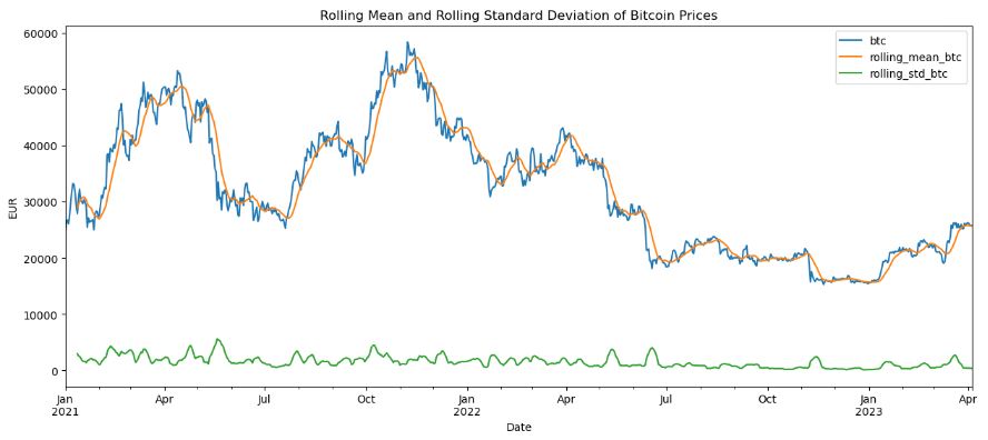
Rolling Mean & Standard Deviation

Let’s plot both rolling mean and standard deviation (STD) of our assets

df1[‘rolling_mean_btc’] = df1.btc.rolling(window=12).mean()
df1[‘rolling_std_btc’] = df1.btc.rolling(window=12).std()
df1.plot(title=’Rolling Mean and Rolling Standard Deviation of Bitcoin Prices’,
figsize=(15,6))
plt.ylabel(“EUR”)
plt.show()

df2[‘rolling_mean_g’] = df2.gold.rolling(window=12).mean()
df2[‘rolling_std_g’] = df2.gold.rolling(window=12).std()
df2.plot(title=’Rolling Mean and Rolling Standard Deviation of Gold Prices’,figsize=(15,5))
plt.ylabel(‘EUR per ounce’)
plt.show()

df3[‘rolling_mean_o’] = df3.oil.rolling(window=12).mean()
df3[‘rolling_std_o’] = df3.oil.rolling(window=12).std()
df3.plot(title=’Rolling Mean and Rolling Standard Deviation of Crude Oil Prices’,
figsize=(15,5))
plt.ylabel(‘EUR per barrel’)
plt.show()

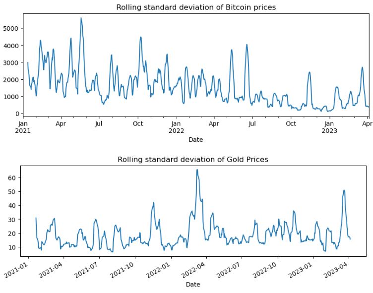
Let’s look at the rolling STD in separated plots

df1[‘rolling_std_btc’].plot(title=’Rolling standard deviation of Bitcoin prices’, figsize=(10,3))
plt.show()
df2[‘rolling_std_g’].plot(title=’Rolling standard deviation of Gold Prices’, figsize=(10,3))
plt.show()
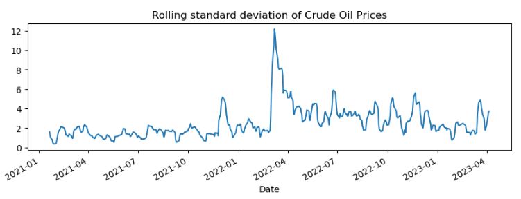
df3[‘rolling_std_o’].plot(title=’Rolling standard deviation of Crude Oil Prices’, figsize=(10,3))
plt.show()

Statistical Analysis Testing & Fitting

Let’s compare ACFs of our assets by omitting the zero lag

fig, ax = plt.subplots(1, 3, figsize=(20,5))

sgt.plot_acf(df1.btc, lags=40, zero=False, ax=ax[0])
sgt.plot_acf(df2.gold, lags=40, zero=False, ax=ax[1])
sgt.plot_acf(df3.oil, lags=40, zero=False, ax=ax[2])
fig.suptitle(‘ACF of Bitcoin (left), Gold (center), and Crude Oil (right) Prices’, fontsize=16)
plt.show()

Let’s run the ADF test

sts.adfuller(df1.btc)

(-1.5503385145013782,
 0.5084790993259574,
 1,
 823,
 {'1%': -3.438320611647225,
  '5%': -2.8650582305072954,
  '10%': -2.568643405981436},
 13734.333273508622)

sts.adfuller(df2.gold)

(-0.8024242489303032,
 0.8184089254307794,
 2,
 567,
 {'1%': -3.441935806025943,
  '5%': -2.8666509204896093,
  '10%': -2.5694919649816947},
 4665.361428783758)

sts.adfuller(df3.oil)

(-1.7540945328321098,
 0.4034786580961352,
 11,
 559,
 {'1%': -3.442102384299813,
  '5%': -2.8667242618524233,
  '10%': -2.569531046591633},
 2449.1714456088794)

Let’s convert prices to log returns

df1[‘log_ret_btc’] = np.log(df1.btc/df1.btc.shift(1))

df2[‘log_ret_g’] = np.log(df2.gold/df2.gold.shift(1))

df3[‘trans_o’] = df3[‘oil’] + 1 – df3[‘oil’].min()
df3[‘log_ret_o’] = np.log(df3.trans_o/df3.trans_o.shift(1))

Check the missing values
print(‘Number of missing values of Bitcoin log returns:’, df1.log_ret_btc.isna().sum())
print(‘Number of missing values of Gold log returns:’, df2.log_ret_g.isna().sum())
print(‘Number of missing values of Crude oil log returns:’, df3.log_ret_o.isna().sum())

Number of missing values of Bitcoin log returns: 1
Number of missing values of Gold log returns: 1
Number of missing values of Crude oil log returns: 1

Let’s plot 3 series of log returns
fig, ax = plt.subplots(3, 1, figsize=(10,9))
df1.log_ret_btc.plot(ax=ax[0])
df2.log_ret_g.plot(ax=ax[1])
df3.log_ret_o.plot(ax=ax[2])
fig.suptitle(‘Bitcoin (top), Gold (middle), and Crude Oil (bottom) Log Returns’, fontsize=16)
plt.show()

Let’s compare the corresponding histograms
fig, ax = plt.subplots(1, 3, figsize=(20,5))
sns.distplot(df1.log_ret_btc[1:], ax=ax[0])
sns.distplot(df2.log_ret_g[1:], ax=ax[1])
sns.distplot(df3.log_ret_o[1:], ax=ax[2])
fig.suptitle(‘Histograms of Log Returns of Bitcoin (left), Gold (middle), and Crude Oil (right)’, fontsize=16)
plt.show()

Let’s check the mean, skewness and kurtosis of log returns
print(‘- Bitcoin log returns:’)
print(‘Mean:’, df1.log_ret_btc.mean())
print(‘Skewness:’, df1.log_ret_btc[1:].skew())
print(‘Kurtosis:’, df1.log_ret_btc[1:].kurtosis())
print(‘\n’)
print(‘- Gold log returns:’)
print(‘Mean:’, df2.log_ret_g.mean())
print(‘Skewness:’, df2.log_ret_g[1:].skew())
print(‘Kurtosis:’, df2.log_ret_g[1:].kurtosis())
print(‘\n’)
print(‘- Crude oil log returns:’, df3.log_ret_o.mean())
print(‘Skewness:’, df3.log_ret_o[1:].skew())
print(‘Kurtosis:’, df3.log_ret_o[1:].kurtosis())

- Bitcoin log returns:
Mean: 7.764716963697599e-05
Skewness: -0.2460688967564316
Kurtosis: 2.771782541387675


- Gold log returns:
Mean: 0.0002631919718611769
Skewness: -0.08269179477267279
Kurtosis: 0.6197039104931932


- Crude oil log returns: 0.006271078632757689
Skewness: 4.001251918715912
Kurtosis: 56.558220392990364

Let’s plot ACFs of log returns without zero lag

fig, ax = plt.subplots(1, 3, figsize=(20,5))

sgt.plot_acf(df1.log_ret_btc[1:], lags=40, zero=False, ax=ax[0])
sgt.plot_acf(df2.log_ret_g[1:], lags=40, zero=False, ax=ax[1])
sgt.plot_acf(df3.log_ret_o[1:], lags=40, zero=False, ax=ax[2])
fig.suptitle(‘ACF of Bitcoin(left), Gold(center), and Crude Oil(right) Log Returns’, fontsize=16)
plt.show()

Let’s perform ARIMA fitting for BTC

import statsmodels.api as sm

model_btc_arma1= sm.tsa.arima.ARIMA(df1.log_ret_btc[1:], order = (1,0,1))
model_btc_arma2= sm.tsa.arima.ARIMA(df1.log_ret_btc[1:], order = (2,0,2))
model_btc_arma3= sm.tsa.arima.ARIMA(df1.log_ret_btc[1:], order = (2,0,1))

results_btc_arma1=model_btc_arma1.fit()
results_btc_arma2=model_btc_arma2.fit()
results_btc_arma3=model_btc_arma3.fit()

print(results_btc_arma1.summary())

print(results_btc_arma2.summary())

print(results_btc_arma3.summary())

print(“ARMA(1,1)”, ‘- AIC:’, results_btc_arma1.aic, ‘, BIC:’, results_btc_arma1.bic)
print(“ARMA(2,2)”, ‘- AIC:’, results_btc_arma2.aic, ‘, BIC:’, results_btc_arma2.bic)
print(“ARMA(2,1)”, ‘- AIC:’, results_btc_arma3.aic, ‘, BIC:’, results_btc_arma3.bic)

ARMA(1,1) - AIC: -3067.8082533837937 , BIC: -3048.951571264156
ARMA(2,2) - AIC: -3067.7282269427815 , BIC: -3039.4432037633246
ARMA(2,1) - AIC: -3065.8293589271334 , BIC: -3042.258506277586

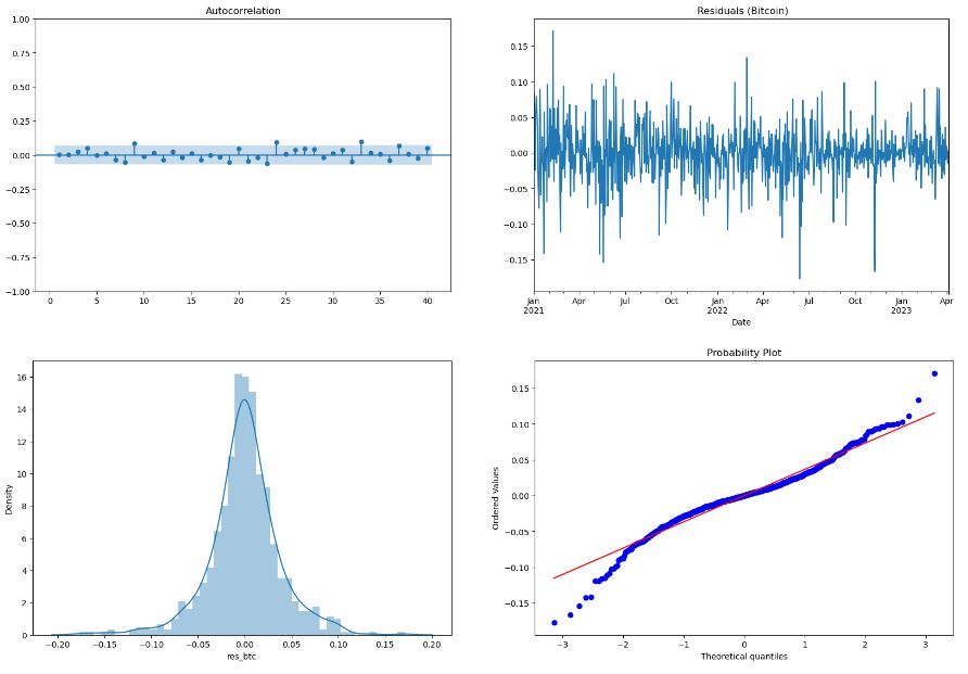
Let’s check ARIMA residuals

df1[‘res_btc’] = results_btc_arima.resid

and plot the QC summary

fig, ax = plt.subplots(1, 2, figsize=(20,6))

sgt.plot_acf(df1.res_btc[1:], lags=40, zero=False, ax=ax[0])

df1.res_btc.plot(title=” Residuals (Bitcoin)”, ax=ax[1])
plt.show()

fig, ax = plt.subplots(1, 2, figsize=(20,6))

sns.distplot(df1.res_btc[1:], ax=ax[0])

scipy.stats.probplot(df1.res_btc[1:], plot=pylab)
pylab.show()

Check the mean of the residual
print(‘Mean of the residuals (Bitcoin):’, df1.res_btc[1:].mean())

Mean of the residuals (Bitcoin): 6.894247743376589e-06

The Shapiro-Wilks test
stats.shapiro(df1.res_btc[1:])

ShapiroResult(statistic=0.9577057957649231, pvalue=1.1367563316978975e-14)

The ARCH test on the squared residuals
het_arch(df1.res_btc[1:]**2, ddof=2)

(6.497558605386769, 0.7718734311025861, 0.647737274525472, 0.773142396367303)

The Ljung-Box test
acorr_ljungbox(df1.res_btc[1:], lags=[30], return_df=True)

30

lb_stat	lb_pvalue
37.342192	0.167379

Risk/Return Optimization

Import libraries:

import math
import scipy.stats as scs
import statsmodels.api as sm
from pylab import mpl, plt
import scipy.optimize as sco
import scipy.interpolate as sci
plt.style.use(‘seaborn’)
mpl.rcParams[‘font.family’] = ‘serif’
%matplotlib inline

Create a data copy

df = data.copy()
df.isna().sum()

BTC-USD       0
CL=F        254
EURUSD=X      0
GC=F        255
btc           0
gold        255
oil         254
dtype: int64

Delete the surplus columns
del df[‘BTC-USD’], df[‘CL=F’], df[‘GC=F’], df[‘EURUSD=X’]
df.dropna(inplace=True)

Create log returns
rets = np.log(df/df.shift(1))
rets.head()

Remove the first missing values
rets.dropna(inplace=True)

rets.isna().sum()

btc     0
gold    0
oil     0
dtype: int64

Rename with tickers for convenience
rets.rename(columns={“btc”: “BTC-EUR”, “gold”: “GC=F”, “oil”: “CL=F”}, inplace=True)

symbols = [‘BTC-EUR’, ‘GC=F’, ‘CL=F’]
noa = len(symbols)

Let’s create the return-volatility table

mean = rets.mean()*252
table1 = pd.DataFrame()
table1[“Annualized Returns”] = mean

std = rets.std()*math.sqrt(252)
table2 = pd.DataFrame()
table2[“Annualized Volatility”] = std

table = pd.concat([table1, table2], axis=1, join=’inner’)
table

Let’s visualize this table
plt.figure(figsize=(8,5))
sns.scatterplot(data=table, x=”Annualized Volatility”, y=”Annualized Returns”, legend=”auto”)
plt.title(‘Risk and Return of Three Assets’)
plt.text(x=table.iloc[0][‘Annualized Volatility’],y=table.iloc[0][‘Annualized Returns’],s=”BTC-EUR”)
plt.text(x=table.iloc[1][‘Annualized Volatility’],y=table.iloc[1][‘Annualized Returns’],s=”GC=F”)
plt.text(x=table.iloc[2][‘Annualized Volatility’],y=table.iloc[2][‘Annualized Returns’],s=”CL=F”)
plt.show()

rets.cov()*252

rets.corr()

Random portfolio weights

weights = np.random.random(noa)
weights /= np.sum(weights)

weights

array([0.63534253, 0.09313641, 0.27152106])

weights.sum()

1.0

Portfolio weighted mean return

np.sum(rets.mean()weights)252

0.07864115142317964

np.dot(weights.T, np.dot(rets.cov()*252, weights))

0.2286568647271813

Dot product weights * rets.cov * weights

math.sqrt(np.dot(weights.T, np.dot(rets.cov()*252, weights)))

0.4781807866562408

def port_ret(weights):
return np.sum(rets.mean() * weights) * 252

def port_vol(weights):
return np.sqrt(np.dot(weights.T, np.dot(rets.cov() * 252, weights)))

Let’s perform 6000 random simulations

prets = []
pvols = []
for p in range (6000):
weights = np.random.random(noa)
weights /= np.sum(weights)
prets.append(port_ret(weights))
pvols.append(port_vol(weights))
prets = np.array(prets)
pvols = np.array(pvols)

Visualization of the Monte Carlo Simulation.
plt.figure(figsize=(10, 6))
plt.scatter(pvols, prets, c=prets / pvols, marker=’o’, cmap=’coolwarm’, edgecolors=’green’)
plt.xlabel(‘Expected Volatility’)
plt.ylabel(‘Expected Return’)
plt.colorbar(label=’Sharpe Ratio’);

Let’s perform optimization

def min_func_sharpe(weights):
return -(port_ret(weights) – 0.0005) / port_vol(weights)

cons = ({‘type’: ‘eq’, ‘fun’: lambda x: np.sum(x) – 1})

bnds = tuple((0, 1) for x in range(noa))
eweights = np.array(noa * [1. / noa,])
eweights

array([0.33333333, 0.33333333, 0.33333333])

Let’s perform the SLSQP minimization

opts = sco.minimize(min_func_sharpe, eweights,
method=’SLSQP’, bounds=bnds,
constraints=cons)

min_func_sharpe(opts.x)

-0.6961516455935085

opts

 fun: -0.6961516455935085
     jac: array([ 0.22786121, -0.00221398, -0.00181666])
 message: 'Optimization terminated successfully'
    nfev: 21
     nit: 5
    njev: 5
  status: 0
 success: True
       x: array([1.80992481e-17, 5.06359696e-01, 4.93640304e-01])

print(f”Optimal Portfolio Weights: {opts[‘x’].round(3)}”)
print(f”Optimal Portfolio Return: {port_ret(opts[‘x’]).round(3)}”)
print(f”Optimal Portfolio Volatility: {port_vol(opts[‘x’]).round(3)}”)
print(‘The maximum Sharpe ratio:’, port_ret(opts[‘x’]) / port_vol(opts[‘x’]))

Optimal Portfolio Weights: [0.    0.506 0.494]
Optimal Portfolio Return: 0.173
Optimal Portfolio Volatility: 0.248
The maximum Sharpe ratio: 0.6981694898420415

optv = sco.minimize(port_vol, eweights, method=’SLSQP’, bounds=bnds, constraints=cons)

optv

 fun: 0.16178844870413478
     jac: array([0.16176193, 0.16179836, 0.16157256])
 message: 'Optimization terminated successfully'
    nfev: 28
     nit: 7
    njev: 7
  status: 0
 success: True
       x: array([0.03486982, 0.92686293, 0.03826725])

mvp_weights = optv.x

print(f”MVP Weights: {optv[‘x’].round(3)}”)
print(f”MVP Return: {port_ret(mvp_weights).round(2)}”)
print(f”MVP Volatility: {port_vol(mvp_weights).round(2)}”)
print(‘Sharpe ratio of MVP:’, port_ret(optv[‘x’])/port_vol(optv[‘x’]))

MVP Weights: [0.035 0.927 0.038]
MVP Return: 0.07
MVP Volatility: 0.16
Sharpe ratio of MVP: 0.4453317527101679

cons = ({‘type’: ‘eq’, ‘fun’: lambda x: port_ret(x) – tret},
{‘type’: ‘eq’, ‘fun’: lambda x: np.sum(x) – 1})

bnds = tuple((0, 1) for x in weights)

trets = np.linspace(0.12, 0.56, 50)
tvols = []
for tret in trets:
res = sco.minimize(port_vol, eweights, method=’SLSQP’, bounds=bnds, constraints=cons)
tvols.append(res[‘fun’])
tvols = np.array(tvols)

Let’s plot the final return-volatility map

plt.figure(figsize=(12, 9))
plt.scatter(pvols, prets, c=prets / pvols, marker=’.’, alpha=0.6, cmap=’coolwarm’)
plt.plot(tvols, trets, ‘b’, lw=3.0)
plt.plot(port_vol(opts[‘x’]), port_ret(opts[‘x’]), ‘y‘, markersize=15.0, label=’Tangency porfolio’) plt.plot(port_vol(optv[‘x’]), port_ret(optv[‘x’]),’r‘, markersize=15.0, label=’Minimum Variance Portfolio’)

plt.legend()
plt.xlabel(‘Expected Volatility’)
plt.ylabel(‘Expected Return’)
plt.colorbar(label=’Sharpe Ratio’)

Summary

• The efficient frontier is formed after the risk-return profile is checked with Monte Carlo simulation, and then the tangential portfolio is the optimal portfolio with the highest Sharpe ratio.
• The expected return and determined volatility are enough to characterize the optimal portfolio
• Other metrics included: Correlation matrix and Sharpe ratio
• The portfolio contains only commodity class (Gold and Oil) which is highly volatile. Most of the budget is spent on the Gold instrument.
• The Sharpe ratio of <1.0 of the tangency portfolio is considered bad, meaning that we are not being compensated very well for the risk we have taken on (return of the portfolio is less the the return of the treasury bills).

Explore More

• Gold ETF Price Prediction using the Bayesian Ridge Linear Regression
• Predicting the JPM Stock Price and Breakouts with Auto ARIMA, FFT, LSTM and Technical Trading Indicators
• Applying a Risk-Aware Portfolio Rebalancing Strategy to ETF, Energy, Pharma, and Aerospace/Defense Stocks in 2023
• SARIMAX X-Validation of EIA Crude Oil Prices Forecast in 2023 – 1. WTI
• SARIMAX-TSA Forecasting, QC and Visualization of E-Commerce Food Delivery Sales
• Portfolio Optimization Risk/Return QC – Positions of Humble Div vs Dividend Glenn
• Algorithmic Testing Stock Portfolios to Optimize the Risk/Reward Ratio
• Stock Portfolio Risk/Return Optimization
• Risk/Return QC via Portfolio Optimization – Current Positions of The Dividend Breeder
• Portfolio max(Return/Risk) Stochastic Optimization of 20 Dividend Growth Stocks
• BTC-USD Freefall vs FB/Meta Prophet 2022-23 Predictions
• Bear vs. Bull Portfolio Risk/Return Optimization QC Analysis

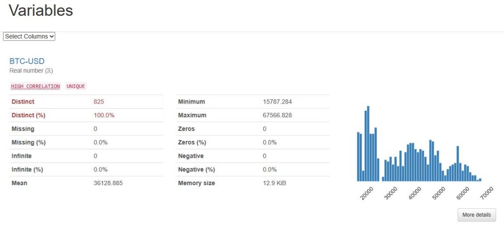
Appendix A: Automated EDA

Let’s create a sweetviz analysis report for our data

import sweetviz as sv
import pandas as pd

report = sv.analyze(data)

report.show_html()

Done! Use ‘show’ commands to display/save.

[100%] 00:00 -> (00:00 left)

Report SWEETVIZ_REPORT.html was generated! NOTEBOOK/COLAB USERS: the web browser MAY not pop up, regardless, the report IS saved in your notebook/colab files.

Let’s use pandas_profiling to generate the html EDA report

import pandas as pd
from pandas_profiling import ProfileReport

profile = ProfileReport(data, title=”Pandas Profiling Report”)
profile.to_file(“report.html”)

Summarize dataset: 100%

30/30 [00:04<00:00, 7.70it/s, Completed]

Generate report structure: 100%

1/1 [00:01<00:00, 1.12s/it]

Render HTML: 100%

1/1 [00:00<00:00, 1.36it/s]

Export report to file: 100%

1/1 [00:00<00:00, 55.56it/s]

Interactions:

Correlations:

Embed Socials

#Risk / #return #stocks #portfolio #optimization
20 #dividend #Growth #StocksToBuy @DrDividend47
vs#SP500 #index #Reference
10k #Stochastic #models #scenarios #performer #riskmanagement #volatility #Awareness #DataScience #ExploreMore #Content 👇🙏https://t.co/C1vi5PSOVF pic.twitter.com/1YzEqpA2af

— Al VA (@alzapress) March 4, 2023

---